F = k(Op Rp)@(Op + Rp)k where Op is the mean luminance in a local 7 x .... Tsotsos et al argue that their model has broader compatibility with the primate visual ...... [36] D. Scott, Multivariate Density Estimation, John Wiley, New York, 1992.
Evolutionary Design for Computational Visual Attention by Neil Douglas Byron Bruce
A thesis presented to the University of Waterloo in fulfilment of the thesis requirement for the degree of Master of Applied Science in Systems Design Engineering
Waterloo, Ontario, Canada, 2003 c Neil Douglas Byron Bruce 2003 °
I hereby declare that I am the sole author of this thesis. This is a true copy of the thesis, including any required final revisions, as accepted by examiners. I understand that my thesis may be made electronically available to the public.
ii
Abstract A new framework for simulating the visual attention system in primates is introduced. The proposed architecture is an abstraction of existing approaches influenced by the work of Koch and Ullman, and Tompa. Each stage of the attentional hierarchy is chosen with consideration for both psychophysics and mathematical optimality. A set of attentional operators are derived that act on basic image channels of intensity, hue and orientation to produce maps representing perceptual importance of each image pixel. The development of such operators is realized within the context of a genetic optimization. The model includes the notion of an information domain where feature maps are transformed to a domain that more closely corresponds to the human visual system. A careful analysis of various issues including feature extraction, density estimation and data fusion is presented within the context of the visual attention problem.
iii
Acknowledgments I thank my supervisor, Dr. Ed Jernigan, for his time and support, both intellectual and financial. In particular, I must thank Dr. Jernigan for a�ording me the opportunity and freedom to explore, and to pursue my personal research interests. Thanks to my readers, Dr. Hamid Tizhoosh and Dr. Catherine Burns, for providing valuable suggestions and insight. To my fellow VIP lab members, and others, for o�ering their time as participants in the experimental work involved in this thesis. To my parents, whose ongoing encouragement and support has given me greater motivation and aspirations. To Chrissie, whose patience, a�ection, and warmth has helped see me through this degree and a�orded me a great deal of happiness. Finally, I recognize with gratitude, the financial support I have received from the Department of Systems Design Engineering and the Ontario Graduate Scholarship program.
iv
Contents 1 Introduction
1
1.1 What is Visual Attention? . . . . . . . . . . . . . . . . . . . . . . .
1
1.2 Neuronal and Physiological Mechanisms . . . . . . . . . . . . . . .
4
1.2.1
Neuronal Mechanisms for Attentional Control . . . . . . . .
4
1.2.2
Saccades . . . . . . . . . . . . . . . . . . . . . . . . . . . . .
5
1.2.3
The Retina and Fovea Centralis . . . . . . . . . . . . . . . .
6
1.3 Control of Attentional Focus and Inhibition of Return . . . . . . . .
8
2 Previous Work
10
3 The Proposed Architecture: A Unifying Framework?
25
3.1 Existing Approaches: Drawing Parallels . . . . . . . . . . . . . . . .
25
3.2 Overview of Proposed Architecture . . . . . . . . . . . . . . . . . .
28
3.3 Design of Nonlinear Attentional Operators: A Genetic Approach . .
32
3.3.1
The Polynomial Framework and Parameter Reduction . . . .
36
3.4 Is a GA an appropriate search technique for the problem ? . . . . .
38
3.5
39
Measures of Self-Information . . . . . . . . . . . . . . . . . . . . . 3.5.1
Center Surround Di�erence . . . . . . . . . . . . . . . . . .
40
3.5.2
Shannon’s Self Information Measure . . . . . . . . . . . . . .
41
v
3.6 On the Fusion of Information Maps . . . . . . . . . . . . . . . . . . 3.6.1
48
Aggregating Belief . . . . . . . . . . . . . . . . . . . . . . .
50
3.7 Eye Tracking Density Maps . . . . . . . . . . . . . . . . . . . . . .
57
3.7.1
Outline of Eye Tracking Experiments . . . . . . . . . . . . .
57
3.7.2
On the Interpretation of Fixation Data . . . . . . . . . . . .
58
3.7.3
Comparing Density and Information Maps . . . . . . . . . .
60
4 Results
61
4.1 Density Estimation . . . . . . . . . . . . . . . . . . . . . . . . . . .
61
4.2 Design of Attentional Operators . . . . . . . . . . . . . . . . . . . .
65
4.3 Fusion of Information Maps . . . . . . . . . . . . . . . . . . . . . .
81
4.3.1
Contrast Adjustment . . . . . . . . . . . . . . . . . . . . . .
81
4.3.2
Ordered Weighted Averages . . . . . . . . . . . . . . . . . .
83
4.3.3
Ordered Weighted Averages with Contrast Adjustment . . .
83
4.3.4
Fuzzy Hybrid Connectives . . . . . . . . . . . . . . . . . . .
85
4.3.5
Fuzzy Integrals . . . . . . . . . . . . . . . . . . . . . . . . .
85
4.3.6
Summary . . . . . . . . . . . . . . . . . . . . . . . . . . . .
93
5 Summary, Limitations and Future Work
102
5.1 Summary . . . . . . . . . . . . . . . . . . . . . . . . . . . . . . . . 102 5.2 Limitations . . . . . . . . . . . . . . . . . . . . . . . . . . . . . . . 104 5.3 Future Work . . . . . . . . . . . . . . . . . . . . . . . . . . . . . . . 105 6 Appendix
112
6.1 Coe!cients for Trained Nonlinear Filters . . . . . . . . . . . . . . . 112
vi
List of Figures 1.1 Flow between key brain regions involved in visual attention. . . . .
5
2.1 The basic framework of the model of Koch and Ullman. . . . . . . .
11
2.2 Two separate images, one textured with a white square the other white with a textured square. In each case attention goes to the smaller square as it displays characteristics unique to the image. . .
15
2.3 Above: A test image to exemplify issues related to Shannon’s measure of self information. Below: The resulting image with a mapping performed based on intensity values. . . . . . . . . . . . . . . . . .
18
2.4 A schematic of the approach based on Shannon’s self information. Note the transition from Fk to Ik is simply the application of Shannon’s self information to the feature map k. . . . . . . . . . . . . .
19
2.5 The model of computational visual attention of Osberger and Maeder. 21 2.6 A schematic of the basic framework of Milanese at al. . . . . . . . .
22
3.1 The proposed architecture for the model outlined in this thesis. . .
30
3.2 Generation of oriented pyramid for production of orientation maps.
32
3.3 The GA framework for the design of nonlinear attentional operators.
36
3.4 Image used for derivation of variance histograms and resulting information maps in example that follows. . . . . . . . . . . . . . . . . .
43
3.5 Left: Histogram derived from local variance measure using 256 bins with bins centered on integer values (top), integers + 0.3 (middle) and using 26 bins rather than 256 (bottom) . Right: Resulting information maps computed using Shannons self information measure as applied to estimate on left hand side in each case. Shown are the midpoints of the histogram bars. . . . . . . . . . . . . . . . . . . . .
44
vii
4.1 Top Middle: A test image to demonstrate the key di�erence between the trained filter and a variance filter. 2nd row: Left: Original image subjected to trained nonlinear filter. Right: Variance image. Bottom: Left: Information map corresponding to nonlinear filtered feature map. Right: Information map corresponding to variance map. 69 4.2 A demonstration of the e�ect of applying the trained nonlinear operator for the intensity map at scale 3. The images shown are (Top to bottom, left to right) The original color image, the intensity map, the intensity map following application of the nonlinear filter, the experimental density map, the distribution of strengths in the feature map, the self information of the feature map, the self information of the nonlinear filtered feature map, the distribution of the nonlinear filtered information map. . . . . . . . . . . . . . . . . . . . . . . . .
70
4.3 A demonstration of the e�ect of applying the trained nonlinear operator for the hue map at scale 3. The images shown are (Top to bottom, left to right) The original color image, the hue map, the intensity map following application of the nonlinear filter, the experimental density map, the distribution of strengths in the feature map, the self information of the feature map, the self information of the nonlinear filtered feature map, the distribution of the nonlinear filtered information map. . . . . . . . . . . . . . . . . . . . . . . . .
71
4.4 Average di�erence between information maps generated using Tompa’s operators and trained nonlinaer operators versus scale. . . . . . . . 73 4.5 From left to right: Top: Original image, experimental density map, average of all information maps. Bottom: Average of intensity information maps, average of hue information maps, average of orientation information maps. Each channel and scale includes an intermediate trained nonlinear filter. . . . . . . . . . . . . . . . . . . . .
74
4.6 From left to right: Top: Original image, experimental density map, average of all information maps. Bottom: Average of intensity information maps, average of hue information maps, average of orientation information maps. Each channel and scale includes an intermediate trained nonlinear filter. . . . . . . . . . . . . . . . . . . . .
75
viii
4.7 From left to right: Top: Original image, experimental density map, average of all information maps. Bottom: Average of intensity information maps, average of hue information maps, average of orientation information maps. Each channel and scale includes an intermediate trained nonlinear filter. . . . . . . . . . . . . . . . . . . . .
76
4.8 From left to right: Top: Original image, experimental density map, average of all information maps. Bottom: Average of intensity information maps, average of hue information maps, average of orientation information maps. Each channel and scale includes an intermediate trained nonlinear filter. . . . . . . . . . . . . . . . . . . . .
77
4.9 From left to right: Top: Original image, experimental density map, average of all information maps. Bottom: Average of intensity information maps, average of hue information maps, average of orientation information maps. Each channel and scale includes an intermediate trained nonlinear filter. . . . . . . . . . . . . . . . . . . . .
78
4.10 Fixations selected by the proposed model for a number of test images. 79 4.11 Fixations selected by the proposed model for a number of images. .
80
4.12 Average score of final combined information map following fusion by contrast adjustment of individual channels and averaging. Shown is the average di�erence between each combined map and density map across the image set for various parameter choices. . . . . . . . . . .
82
4.13 Average score of final combined information map following fusion by applying the Schweizer and Sklar norm across each channel. Shown is the average di�erence between each combined map and density map across the image set for various parameter choices. . . . . . . .
87
4.14 Average score of final combined information map following fusion by applying the Schweizer and Sklar co-norm across each channel. Shown is the average di�erence between each combined map and density map across the image set for various parameter choices. . .
88
4.15 Average score of final combined information map following fusion by applying the Yager norm across each channel. Shown is the average di�erence between each combined map and density map across the image set for various parameter choices. . . . . . . . . . . . . . . . .
89
4.16 Average score of final combined information map following fusion by applying the Yager co-norm across each channel. Shown is the average di�erence between each combined map and density map across the image set for various parameter choices. . . . . . . . . . . . . .
90
ix
4.17 Average score of final combined information map following fusion by applying the Hamacher norm across each channel. Shown is the average di�erence between each combined map and density map across the image set for various parameter choices. . . . . . . . . . . . . .
91
4.18 Average score of final combined information map following fusion by applying the Hamacher co-norm across each channel. Shown is the average di�erence between each combined map and density map across the image set for various parameter choices. . . . . . . . . . .
92
4.19 A comparison of various fusion strategies. From top to bottom, left to right are: Original Image, experimental density map, average, contrast adjustment, OWA, OWA+contrast adjust, Schweizer and Sklar norm, Hamacher norm, Yager norm. . . . . . . . . . . . . . .
97
4.20 A comparison of various fusion strategies. From top to bottom, left to right are: Original Image, experimental density map, average, contrast adjustment, OWA, OWA+contrast adjust, Schweizer and Sklar norm, Hamacher norm, Yager norm. . . . . . . . . . . . . . .
98
4.21 A comparison of various fusion strategies. From top to bottom, left to right are: Original Image, experimental density map, average, contrast adjustment, OWA, OWA+contrast adjust, Schweizer and Sklar norm, Hamacher norm, Yager norm. . . . . . . . . . . . . . .
99
4.22 A comparison of various fusion strategies. From top to bottom, left to right are: Original Image, experimental density map, average, contrast adjustment, OWA, OWA+contrast adjust, Schweizer and Sklar norm, Hamacher norm, Yager norm. . . . . . . . . . . . . . . 100 4.23 The best overall model applied to some di!cult and less usual images. Predicted regions of highest interest are circled in yellow. . . . 101
x
List of Tables 3.1 Various popular choices for Kernel Windows. . . . . . . . . . . . . .
46
3.2 Particular parameter choices for the OWA operator. . . . . . . . . .
51
3.3 Special cases of the Sugeno integral. . . . . . . . . . . . . . . . . . .
54
3.4 Special cases of the Choquet integral. . . . . . . . . . . . . . . . . .
54
3.5 Some simple t-norms and associated t-conorms. . . . . . . . . . . .
56
3.6 t-norms and t-conorms of the parameterized variety. . . . . . . . . .
57
4.1 Average histogram density estimator di�erence values for image at scale 1 (340x256). . . . . . . . . . . . . . . . . . . . . . . . . . . . .
61
4.2 Average histogram density estimator di�erence values for image at scale 2 (170x128). . . . . . . . . . . . . . . . . . . . . . . . . . . . .
62
4.3 Average histogram density estimator di�erence values for image at scale 3 (85x64). . . . . . . . . . . . . . . . . . . . . . . . . . . . . .
62
4.4 Average histogram density estimator di�erence values for image at scale 4 (42x32). . . . . . . . . . . . . . . . . . . . . . . . . . . . . .
62
4.5 Average kernal density estimator di�erence values for image at scale 1 (340x256). . . . . . . . . . . . . . . . . . . . . . . . . . . . . . . .
63
4.6 Average kernel density estimator di�erence values for image at scale 2 (170x128). . . . . . . . . . . . . . . . . . . . . . . . . . . . . . . .
63
4.7 Average kernel density estimator di�erence values for image at scale 3 (85x64). . . . . . . . . . . . . . . . . . . . . . . . . . . . . . . . .
63
4.8 Average kernel density estimator di�erence values for image at scale 4 (42x32). . . . . . . . . . . . . . . . . . . . . . . . . . . . . . . . .
64
xi
4.9 Numeric score of the trained operators verus some of Tompa’s choices. Numbers indicated the average absolute error between the two density distributions across all images in the test set. . . . . . . . . . .
72
4.10 Average score of final combined information map following ordered weighted averaging. Shown is the average di�erence between each combined map and density map across the image set for various parameter choices. . . . . . . . . . . . . . . . . . . . . . . . . . . .
84
4.11 Average score of final combined information map followining contrast adjustment of individual channels (power of 3.8) followed by ordered weighted averaging. Shown is the average di�erence between each combined map and density map across the image set for various parameter choices. . . . . . . . . . . . . . . . . . . . . . . . . . . .
86
4.12 Average score of final combined information map following fusion using the various approaches. In each case the best choice of parameters is used. . . . . . . . . . . . . . . . . . . . . . . . . . . . . . . .
96
xii
Chapter 1 Introduction 1.1
What is Visual Attention?
The perceptual information available to a human at any given moment is vast. In particular, humans receive a great quantity of information through the human visual system and are able form a mental model of a scene in a seemingly instantaneous manner. The basic essence of attention is perhaps best captured by James[1]: "Every one knows what attention is. It is the taking possession by the mind, in clear and vivid form, of one out of what seem several simultaneously possible objects or trains of thought. Focalization, concentration, of consciousness are of its essence. It implies withdrawal from some things in order to deal e�ectively with others". Although this encapsulates the basic idea of what is meant by attention, a more exact description taking into account neurobiological facets of attention is imperative for the purposes of the work presented in this thesis. A substantial amount of e�ort has been devoted to learning about the human visual system, although we are 1
still far from having a complete neurobiological understanding. Much however is known regarding the physiology of the eye and di�erent components of the human imaging system.[2] The human visual system consists of three chief components critical to attention: i.
Eye movements called saccades
ii. A foveal gradient of resolution iii. Neural processing on the retina Details of components ii. and iii. are left to section 1.2. An understanding of i., saccadic eye movement, is a necessary condition on understanding what is meant by visual attention and the importance of visual attention. In a comprehensive study[3] Yarbus showed that the perception of a scene involves a complex sequence of saccades, where the eye jumps quickly to foveate a new part of the scene, and fixations, where the eye remains still. The points that one fixates in a scene tend to be those that are critical to forming an understanding of the scene[4]. One issue that remains controversial is whether movement of the eyes is controlled by the goal of an observer or by attracting stimuli. A variety of studies focusing on this issue have taken place in the past 3-4 decades[5]. Perhaps the most influential of these studies is that of Yarbus[3] who determined that the scanpath of an observer when viewing an image is influenced by the question posed by the experimenter prior to viewing. However, although the scanpath varied greatly depending on the question asked, the set of fixation points was quite consistent across all subjects suggesting that stimulus and not a supposed goal determines the points on which one has a tendency to fixate. A couple of other studies also provide evidence for 2
this same supposition. One such study determined that features in an image tend to attract an observer’s gaze away from planned paths.[6] Subjects were asked to scan across the image in the same manner that one might view a page of text. In doing so, it was found that the viewers gaze would pause while passing over lines perpendicular to the planned route. In this case, the goal of the observer was dominated by the e�ect of stimulus. Another example is that of a study measuring eye movements of radiologists when viewing chest x-rays. It was determined that in 70 to 90 percent of cases where a tumor was missed, the eyes of the radiologist fixated the location of the the missed tumor.[7] In this case, because the eyes of the observer were drawn to the tumor without having recognized its presence, it follows that the movement of the eyes to the location of the tumor must have been driven by stimulus in the locality of the tumor rather than cognitive information. Most literature now subscribes to the idea that attention involves two functionally independent components: An early pre-attentive stage in which eye movements are purely stimulus driven and help in the creation of a mental model of a scene, and an attentive stage, in which a series of fixations are followed to process the formed model bearing in mind a supposed goal[8]. In this thesis we are interested in the pre-attentive stage in which saccadic eye movements are driven entirely by stimulus facilitating the processing of the vast quantity of information that enters the visual sensory pipeline. Visual attention in the remainder of this thesis refers to the early pre-attentive visual process by which a mental model of a scene is conceived. The process is assumed entirely stimulus driven and the goal of this thesis is that of producing a computational approach to emulate the process of visual attention in humans. 3
1.2
Neuronal and Physiological Mechanisms
1.2.1
Neuronal Mechanisms for Attentional Control
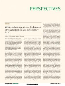
An understanding of the neurophysiology of attention appears to be quite important in producing a model of visual attention that adheres to psychophysical considerations. A number of regions of the brain participate in early visual attention. Key regions of the brain include the visual cortex, inferotemporal cortex, posterior parietal cortex, prefrontal cortex and superior colliculus.[9] The flow of visual information between these regions of the brain is seen in Figure 1.1. Information enters the visual pipeline via the visual cortex and then proceeds along two parallel pathways. The two pathways include a dorsal stream and a ventral stream. The dorsal stream includes the posterior parietal cortex and its primary task is that of focusing attention on regions or objects of interest in a scene. The ventral stream including the inferotemporal cortex is responsible for identification and recognition tasks. Although the ventral stream is not directly involved in attention, these regions of the brain have been shown to receive attentional feedback and are responsible for establishing a mental representation of objects and locations that one attends to. The aforementioned neuronal structure provides strong evidence in favor of a low-level attentional mechanism responsible for localization coupled with a higher-level component facilitating object and scene representation as well as identification. This framework strongly suggests that attention consists of a task independent component that focuses later processing. The prefrontal cortex is bidirectionally connected to both the inferotemporal cortex and posterior parietal cortex and controls eye movement through the superior colliculus as well as 4
Figure 1.1: Flow between key brain regions involved in visual attention. modulating the dorsal and ventral processing streams.
1.2.2
Saccades
Saccades are quick, jumpy eye movements that may result from voluntary movement or reflex control. A voluntary saccade might happen if one is told to look in a particular direction or at a particular target. In contrast, a reflex saccade may
5
occur as a result of sudden movement, or vibrant color when one first encounters a scene. In response to such stimuli, the human ocular motor system will position the eyes in the locality of strong stimulus following a latency of approximately 225 msec. The peak movement velocity and the duration of the saccade are dependent on the distance that the eye moves, varying from 30 to 700 degrees/second with movements ranging from 0.5 degrees to 40 degrees in amplitude. After a required delay, the saccadic reaction to stimulus in the image involves an interval of acceleration of the eyes to a peak velocity followed by deceleration onto the new target position. The purpose of saccades is that of collecting information regarding salient portions of a scene for further high-level processing. Saccades direct the processing of information in a scene, collecting detailed high resolution information from conspicuous localities while ignoring areas of little interest.[4]
1.2.3
The Retina and Fovea Centralis
The Retina
The retina consists of a light-sensitive tissue layer at the rear of the eye that covers approximately 65 percent of its inner surface. The center of the retina contains a small area called the fovea or fovea centralis. This area is the area in which the eye’s vision is most acute. The fovea is approximately 1 degree in diameter and visual acuity drops sharply outside the fovea. The retina contains photosensitive cells called rods and cones that transform incoming light energy into signals that travel to the brain through the optic nerve. Approximately 125 million rods and cones are distributed nonuniformly over the surface of the retina. The role of rods 6
might be compared to that of high-speed black and white film. The array of rods is able to perform in light too dim for the cones to handle, unable to resolve color and relays images that are not very well defined[10]. In contrast, the cones give detailed colored views in brighter light, somewhat analagous to low-speed color film.
The Fovea Centralis
The field of view over which humans receive data is about 200 degrees, however, the resolution over most of that field is rather coarse. To capture high resolution data on an image, the light must land on the fovea centralis, reducing the region of sharp vision to around 15 degrees. In lower light, as no rods are located on the fovea, the fovea is e�ectively blind. The most acute vision in the dark lies approximately 8 degrees from the center of the fovea. In the center of the retina, there is a small region about 1.5 m in radius termed the macula. In the center of the macula is the fovea centralis, a region of 0.15 mm radius.[10] The fovea centralis is very high in cones and contains no rods. The cones on the fovea are thinner and far more densely packed than elsewhere on the retina. Eye Fixations As the fovea captures information of the highest detail, the eye moves around quickly to areas containing certain stimuli so that light from a region of interest falls directly on the fovea. Regions to which the eyes are drawn through a reflex eye movement are typically areas in which something with a distinct characteristic
7
is located. For example, a bright red bird on a tree has a unique color in the scene and for that reason is likely to draw attention from an observer. Perception of a scene is fabricated by continuous analysis by the brain of the time-varing image captured on the retina.
1.3
Control of Attentional Focus and Inhibition of Return
From a computational viewpoint, often the goal of including an attentive stage is that of reducing processing on the whole image to processing of a sequence of salient circumscribed regions. In the context of computational visual attention, this most often requires a mechanism for going from a computed salience map to a series of points representing foveated regions of interest. Although the focus of the work here is that of coming up with the salience map that precedes this stage, it is nevertheless worth briefly mentioning a plausible architecture for this step. One architecture that has gained support in recent years is that of a winner-takeall network[11][12] which serves as a neurally based detector of a maximum. To avoid focusing on a single maximum, neurons in the locality of the attended region are inhibited to allow choice of a new gazepoint. This strategy allows sequential selection of gazepoints and associated scanpaths. This approach has been applied successfully to applications such as video transmission, image compression, and mobile robot navigation[13]. It should be noted that in some cases, it is possible to employ the salience map directly to facilitate a perceptually motivated task. For instance, salience maps have been applied to perceptually motivated measures of 8
image quality[14].
9
Chapter 2 Previous Work
One of the first neurally credible frameworks for simulating human visual attention was proposed by Koch and Ullman[11] in 1985. Their model focused on the idea of a ’saliency map’ which they define as a two-dimensional topographic representation of conspicuity for every pixel in the image. Their proposed model consisted of 4 key steps: Low-level feature extraction, centre-surround di�erences to produce feature maps, combination of feature maps, and finally, attentional selection and inhibition of return. Figure 2.1 shows the key steps of the Koch and Ullman model. As can be seen, the approach revolves around early extraction of primitive features followed by an operator that is given by the di�erence between the measured feature strength of each pixel and surrounding strengths to produce feature maps. The feature maps are then combined to produce a saliency map that facilitates the selection of localized image regions for further processing. Much examination of this model has been performed in the last 15 years including close examination of various components of the model by Koch, Ullman and additionally Niebur and Itti[15]. Some of the ideas that come out of the Koch and Ullman framework contribute 10
Figure 2.1: The basic framework of the model of Koch and Ullman.
11
to the work presented in this thesis and are discussed in more detail in chapter 3. The feature extraction stage involves the computation of orientation, colour and intensity maps at 6 spatial scales with downscaled maps computed using the Burt and Adelson gaussian pyramid scheme which consists of progressive low-pass filtering and subsampling[16]. This step is followed by a center surround di�erence operator in which the center of the receptive field is given by a pixel at level f 5 {2> 3> 4} of the Gaussian pyramid and the surround by the corresponding pixel at level v = f + � with � 5 {3> 4} giving 6 feature maps at scales 2-5,2-6,3-6,3-7,4-7 and 4-8 for each type of feature. Across scale di�erence between maps is performed through interpolation to the finer scale and subtraction. This scheme is used in lieu of a single center surround operator to lessen the dependence of the center surround mask size on scale. Intensity maps are computed as the average of the red, green and blue values for each pixel. Two colour feature maps were computed using the centre surround operator at each of the six scales. The first of the colour feature maps is given by the (red-green) value in the centre minus the (green-red) value in the surround followed by an absolute value. To derive the second blue/yellow feature maps with yellow given by the average of the red and green channels the same set of operations are performed. The orientation maps are computed using oriented gabor filters for four separate orientations(0,45,90,135)[17]. In total there are 24 orientation maps corresponding to the four orientations at 6 spatial scales, 12 colour maps given by the two di�erent colour channels at 6 spatial scales and lastly 6 intensity maps. The feature maps derived from these 42 maps through the center surround operator were then combined through a weighted average. Another well-known study on the issue of visual attention is that of Privitera 12
and Stark[18]. Privitera and Stark evaluated numerous algorithmic approaches to detecting regions of interest by comparing the output of such algorithms to eye tracking data captured using standard eye tracking apparatus. Privitera and Stark compared 10 di�erent algorithmic methods for detecting regions of interest: 1. The Canny operator, which measures edges per unit area[19]. 2. High curvature masks incorporating both varying orientations of acute angles as well as an "X" shaped mask. 3. A 7 x 7 centre-surround mask including positive centre and negative surround similar to that in the model of Koch and Ullman. 4.
Gabor masks to measure grey-level orientation di�erences based on the
model of Niebur and Koch.[20]. The orientation vector was defined as a weighted sum of the various responses to arrive at an average orientation vector. 5. A discrete wavelet transform based on the Daubechies and Symlet bases using a pyramidal scheme. 6. A measure of local symmetry. 7. Michaelson contrast[21] defined as: F = k(Op � Rp )@(Op + Rp )k where Op is the mean luminance in a local 7 x 7 neighborhood and Rp the overall mean luminance. 8. An entropy measure of the type often used to measure texture variance given by:
Q=
X
il log il
lMJ
13
(2.1)
where il is the number of times the ith grey level occurs in the image. 9. Coe!cients of the Discrete Cosine Transform with high frequency components indicating areas of interest. 10. The Laplacian of the Gaussian, which Marr suggested as having some correlation to visual regions of interest.[22] Privitera and Stark found that each of the 10 operators with the exception of the discrete cosine transform showed a strong correlation to measured fixations for some of the images but performed quite poorly for others. This result suggests that no single measure can predict the location of every region of interest. This is a quality that seems to have given the Itti and Koch model a step up on on some of the approaches that are based on a single property. In 1991, Topper[5] introduced an interesting addition to the visual attention literature. The premise of his work is as follows: Strength of a particular feature in an area of the image does not in itself guarantee that ones attention will be drawn to that image area. Consider figure 2.1, shown are two separate cases, one in which attention tends to go to a region with many edges and the other where attention tends to go to a more homogeneous area. It is clear that a detector based on edges would fail miserably on this set of two images. What is evident, is the fact that attention is drawn to an area of the image in which a certain quality is di�erent than the rest of the image. Topper’s idea was to transform a set of measured feature maps to a more perceptually relevant domain through an operator that measures the uniqueness of each feature strength relative to other strengths. Owing to the close ties between this 14
Figure 2.2: Two separate images, one textured with a white square the other white with a textured square. In each case attention goes to the smaller square as it displays characteristics unique to the image.
15
premise and ideas that come out of information theory, Topper suggested Shannon’s measure of self information as an appropriate transform. In the context of this problem, Shannon’s measure of self information may be described as follows. The premise of Shannon’s measure is the idea that the information conveyed by an event is inversely proportional to the probability of the event occurring. Intuitively, this assertion seems valid and may be made more lucid in the context of an example. If one is gazing at the ceiling of a room and the entire ceiling is homogeneous with the exception of a light fixture, one’s attention will tend to be drawn to the light fixture. In a di�erent light, if a small portion of the ceiling is chosen at random, the probability that the piece is part of the homogenous ceiling is far higher than it belonging to the light fixture. Based on this observation, Shannon’s model predicts that a portion of the light fixture contains more useful information than a blank region of the ceiling. It is this idea that makes Shannon’s self-information measure a useful tool in predicting regions of an image that are informative or of interest. Shannon suggested the log operator, L({) = log(1@S ({)) as the best operator to produce the desired inverse proportionality while allowing for a few important considerations. First, an event that will definitely occur (S ({) = 1) conveys no information (L({) = 0), this consideration is preserved when using the log operator. Second, if S ({) = 0, the information conveyed by such an event should be undefined. This is a non-issue since an event of probability zero will never occur but mathematically, the log operator handles this detail. A third important property of the transformation is that of additivity. That is, if S ({ _ |) = S ({) S (|) then it follows that L({ _ |) = L (S ({)S (|)) = � log S ({) � log S (|) = L ({) + L (|). This is an important consideration in checking for redundant feature definitions. It 16
would likely be instructive to provide an example of the application of Shannon’s self-information measure within the context of our visual attention problem. Consider the two images shown in figure 2.2: The top image is the original and the second is the result of applying Shannon’s information measure to the top image. In this case, P(x) is defined to be the probability density of pixels of intensity x and each pixel is mapped to a new value using the definition L({) = log(1@S ({))= The utility of Shannon’s measure is evident in this simple case with the smaller squares, which seem to draw attention, receiving greater confidence values. In the second image, the intensity value receiving the highest information measure in the original is mapped to white in the output. Others are given a value between black and white based on the ratio of their respective information measures to this maximum. This convention has been assumed in all images of this nature unless otherwise stated. The behaviour of this information operator is consistent with psychophysics, in that humans tend to be drawn to areas of the scene that contrast with the rest of the scene[1]. Topper performed a set of experiments along the same lines as those of Privitera and Stark. He measured the correlation of feature maps to eye tracking density maps following the application of Shannon’s self information measure to the feature maps. As in the case of Privitera and Stark, the correlation for each operator was substantial in some cases and worse in others. Perhaps the most important result from his work was that the self-information operator allowed the detection of regions of interest that would never be detected by a strict measure on the image. Tompa[23] introduced an approach to computational visual attention based on 17
Figure 2.3: Above: A test image to exemplify issues related to Shannon’s measure of self information. Below: The resulting image with a mapping performed based on intensity values.
18
Figure 2.4: A schematic of the approach based on Shannon’s self information. Note the transition from Fk to Ik is simply the application of Shannon’s self information to the feature map k. a subset of the measures employed by Topper for which the correlation to density maps was seen to be particularly strong. The information maps derived from this feature subset were then integrated by means of a few elementary operators (min,max,product,sum and sum of squares) to derive an overall perceptual importance map. Figure 2.4 provides a schematic for the approach used in Tompa’s work. The model shown in figure 2.4, along with the model of Koch and Ullman establishes a foundation for the model developed in this thesis.
Tompa’s model involves three key components: The first component is the derivation of feature maps from the original image. The 6 operators used in Tompa’s approach are Sobel edge magnitude, Sobel edge orientation, intensity, hue, variance, 19
and moment of inertia. These measures were observed to have the strongest correlation to eye tracking results in Topper’s work. The next stage consists of computing information maps through the application of Shannon’s self information measure to the feature maps. This was done in the same manner prescribed by Topper in his thesis. The last stage consists of combining the information maps to arrive at a final importance map. Tompa tried various simple approaches including taking the average, sum of squares, minimum, and maximum of the 6 maps. The sum of squares operator was found on average to provide the best results. The approaches of Koch and Ullman, Privitera and Stark, Topper, and Tompa have been outlined in some detail as they comprise necessary background for some of the sections that follow. Numerous other approaches to the problem of computational visual attention have been taken that have a less direct connection to the work presented in this thesis. Nevertheless, in the interest of completeness a mention of some of these other approaches would likely be of benefit. Osberger and Maeder[24][25] present an approach that involves segmentation of the image using a recursive split and merge algorithm. During segmentation, regions of fewer than 16 pixels are merged with the most similar neighbor. Segmented regions are then assigned importance values according to five criteria. A basic schematic of the approach employed by Osberger and Maeder is seen in figure 2.5. The five measures that are performed on the segmented image are as follows: 1. A contrast measure given by the di�erence between the mean intensity of each region and the mean intensity of surrounding regions. 20
Figure 2.5: The model of computational visual attention of Osberger and Maeder. 2. Size, the number of pixels making up the region. 3. A shape value computed as the ratio of pixels on the border to pixels making up the entire region. 4. Location, given by the number of region pixels that fall within the central quarter of the image with more central regions favoured. 5. Background, given by the number of region pixels on the edge of the image with higher values being unfavourable.
All feature measures are normalized to lie between 0 and 1 such that 1 always indicates greatest confidence that a pixel is important while 0 is is the least favourable level of confidence a pixel may receive. Factors are combined by summing the squares of the confidence values derived from the 5 feature measures to give a single importance measure to each region. The success of their approach 21
Figure 2.6: A schematic of the basic framework of Milanese at al. has been found to depend highly on the performance of the segmentation and the approach has virtually no psychophysical evidence for support and little theoretical basis. Milanese et al.[26][27][28] use two groups of features to derive feature maps as the basis for their model. The two groups of features include contours and regions. Contour measures include measures of contrast, curvature, length and orientation of contours in the image. Region measures include perimeter, grey level, area and elongation. Figure 2.5 illustrates the chief components of the approach of Milanese et al. Similar to the information domain methods and centre surround di�erences, they employ a mapping on the feature maps to arrive at conspicuity maps. The transformation that carries out this operation is as follows:
n = Fl>m
X ¯ ¯ 1 n n ¯ ¯Il>m � Ip>q kQl>m k p>qMQ l>m
22
(2.2)
with the F’s being measured values in the feature maps and N the local neighbourhood of the operator. Resulting conspicuity maps are combined using a somewhat ad hoc relaxation operation. The model of Milanese et al., like the model of Osberger and Maeder lacks a psychophysical backing and contains some steps that seem to be chosen rather arbitrarily. Tsotsos et al.[29] proposed an attentional selection strategy that employs the combination of a bottom-up feature extraction hierarchy with selective tuning of the feature extraction mechanisms through feedback within a pyramidal processing architecture. The target region of interest is chosen through feedforward activation at the top level of the processing hierarchy(Equivalent to an importance map) through a top-down hierarchical winner-take-all process. Spatial competition for saliency is then modified at each level of the WTA hierarchy as feed forward connections that do not play a role in the choice of the winning locality are pruned. The result of this feedback propagation through the pyramid of winner-take-all networks is that of an inhibitory beam around the chosen area of interest. Tsotsos et al argue that their model has broader compatibility with the primate visual system than any competing approach. This approach is in a slightly di�erent light than some of the others but does have some parallels to the approach of Koch et al.[30] It is clear that a variety of di�erent approaches have been taken to deal with simulating visual attention in primates. One might notice that all of these models seem to have common elements. All of them involve some form of low level extraction of features on the image. Most involve some transformation from these measured feature maps to maps that more closely resemble a representation of perceptual 23
relevance. Combining maps representing importance also seems to be a common element in most of these models. One begins to get the sense that although numerous approaches to the problem have been taken, there is a fundamental similarity between many of the models regardless of whether they are derived through psychophysical principles or for purely mathematical reasons. This observation is a part of the motivation of the model that is developed in this thesis. Recognizing that common elements exist should allow abstraction to a more general model that encompasses ideas from a variety of the leading approaches that currently exist.
24
Chapter 3 The Proposed Architecture: A Unifying Framework? 3.1
Existing Approaches: Drawing Parallels
One of the more recent proposed approaches to computational visual attention is that of Tompa.[23] To reiterate briefly the description in the previous chapter, Tompa proposed a framework that revolves around the notion of an information domain, first introduced within the context of visual attention by Topper.[5] Tompa’s framework involved taking 6 local feature measures on the RGB image such as edge strength, variance and hue, followed by an operation quantifying the uniqueness of the feature strength assigned to each pixel. This operation, based on Shannon’s measure of self information brings each feature map into the information domain, a domain that corresponds more closely to the perceptual domain. The resulting information maps were then combined by summing the squares of the resulting strengths in the information maps across each map. The work for this thesis began as a closer analysis of the model of Tompa. In particular there are three distinct 25
components in the model of Tompa that require careful analysis. The first is the issue of how the information maps are combined. The second issue is in estimating the density of strengths in the feature map when performing the self-information measure. Lastly, the operators chosen by Tompa were chosen from a larger set of well-known operators on the basis that subject to a self-information measure, the information maps based on these 6 features came closest to eye tracking density maps across a set of images. Although the measures were chosen from a larger set of operators, the set of operators from which Tompa’s choices were made represents only an infinitesimal fraction of the operators that might be chosen from a nonlinear function space. For this reason, it is reasonable to assume that one might do better in choosing operators through an appropriately designed optimization, from a larger subspace of the non-linear function space than the dozen or so operators that Tompa chose from. One of the ambitions of the work is to derive a set of attentional operators on the image space from a space of operators that includes all possibilities from the work of Tompa. Clearly, to choose a set of operators from the entire space of non-linear functions yields a problem that is ill-defined. More realistic would be the selection of an operator set from a smaller subspace defined by a suitably chosen framework. However, the edge orientation map and hue map in his approach are derived from inverse trigonometric operators on the RGB color channels. The other four operations are all readily derived from the RGB channels using an appropriate first or second order operator. Selecting a framework for a nonlinear operator that acts on the RGB channels and arrives at all of the operators that Tompa employed does not appear realizable in any simple form. For this reason, the following is proposed: The image is initially broken down into three separate 26
carefully chosen channels; operators that act on each of the channels separately are then derived and applied to the respective channels. The three most basic measures that seem to allow the derivation of all the operators from Tompa’s study through an appropriate optimization within a relatively simplistic framework are: intensity, hue and orientation. The 6 operators employed by Tompa may be derived from these choices through simple 1st and 2nd order polynomial filters. Those familiar with the visual attention literature may notice something curious about this set of primitives: These three basic primitives chosen to allow an optimization that includes all of the operators employed in Tompa’s study are the same three chosen for psychophysical reasons by Nieber, Itti and Koch in perhaps the most famous of computational visual attention systems. Interesting is the fact that Tompa who chose operators based on correlation to eye tracking results happened to choose a set of operators based on primitives that may be arrived at through a choice made purely under psychophysical considerations. Further, it becomes evident when examining the model of Tompa from this vantage point that the two models essentially di�er only in the replacement of center-surround di�erences and normalization in the model of Itti, Niebur and Koch with suitable non-linear operators followed by a self-information measure in Tompa’s model. One might go as far as saying that the center surround di�erence is essentially a measure of self-information of local extent. The fact that very di�erent means were employed to arrive at the two final models and that these two models may be shown fundamentally equivalent provides a strong case for the feature measure / self-information framework. One might regard the goal of this thesis as a closer examination of the approach of Tompa. One might also regard this approach as an variation on the framework of 27
Niebur, Itti and Koch. The two aforementioned approaches are essentially subsets of a common, more general model. Each component of this more general model will be chosen with due care and consideration of measured eye tracking density results. One of the main goals of this thesis is to derive a set of nonlinear operators to act on the three basic channels, modeled within the context of a local extent quadratic Volterra filter, that lies between the image primitive stage and the self-information stage. The operators will be selected in such a way that correlation to eye tracking density maps is optimized at each stage of the process. Issues of scale will be dealt with in the same manner as the Niebur, Itti and Koch study. The proposed framework, an abstraction of the two aforementioned models, is described in more detail in the section that follows along with a comparison of components in the Itti, Koch et al. model with components in the model of Tompa.
3.2
Overview of Proposed Architecture
As mentioned in the previous section, the proposed architecture is intended to serve as an abstraction of the models of Koch and Ullman, and Tompa. In this section, the proposed model will be described along with how the Koch and Ullman and Tompa models fit into the proposed architecture. The proposed framework consists of 4 key components: 1. An early feature extraction phase in which the initial RGB image is divided into an intensity channel, a hue channel and 4 orientation channels using oriented gabor filters as is the case in the Koch and Ullman model. A channel for each of 28
these images will be produced at 4 spatial scales in the same manner employed in the Itti and Koch approach. 2. A set of non-linear functions that act on the primitive channels (intensity, hue, and orientation) to derive higher-level measures. For example, mapping to a variance map or an edge map from the intensity channel in the case of Tompa’s approach. In this case, the non-linear functions will be produced by a GA training procedure and hence can not be named explicitly as in Tompa’s model as they are not well known measures. The maps resulting from this operation shall be referred to as attention maps as the non-linear operators are designed as a measure on the image that represents attention. It is clear why a measure such as variance might hint at areas that will draw attention but it is expected that some other operator designed specifically for this purpose might do far better. 3. An information operator that takes each higher-level map to a domain that more accurately represents human perception called an information map as outlined in chapter 2. This stage is the centre surround di�erence in the Koch and Ullman model and the Shannon self-information measure in Tompa’s model. 4. Combination of the information maps derived in step 3 to arrive at an overall perceptual importance map. A schematic of this framework is depicted in figure 3.1.The steps involved in the feature extraction stage are straightforward. The intensity channel is derived as the average of the red, green and blue values corresponding to each pixel. The hue channel is given by K = � if E ? J, K = 2� � � if E � J where � = 0=5[(U3J)+(U3E)] arccos [(U3J) 2 +(U3E)(J3E)]0=5 and U> J and E are the red, green and blue values
29
Figure 3.1: The proposed architecture for the model outlined in this thesis.
30
corresponding to each pixel. The orientation channel is derived using overcomplete steerable pyramid filters[17] as was the case in the model of Itti and Koch. Figure 3.2 outlines the oriented pyramid generation. The image in the Laplacian pyramid at level n is given by: Lq =Gq -Gq+1 where Gq and Gq+1 represent the nwk and (n+1)wk levels of the gaussian pyramid[16]. Subtraction happens before the (n+1)wk level is subsampled. The oriented pyramid is then constructed by modulating each level of the Laplacian pyramid with the following four complex sinusoids: I
p1 ({> |) = hl(�@2){ ; p2 ({> |) = hl(I2�@4)({+|) p3 ({> |) = hl(�@2)| ; p4 ({> |) = hl( 2�@4)(|3{)
(3.1)
Following this step, each level of the Laplacian pyramid has e�ectively been convolved with a set of log-Gabor filters:
[n ({> |) =
1 3({2 +|2 )@2 h pn ({> |); n = 1==4 2�
(3.2)
Power maps are given by the sum of squares of the real and imaginary parts generated in this previous step. The second step involves the application of a non-linear operator to each of the basic channels. The manner in which these non-linear operators are derived is detailed in the section that follows. For the self-information stage, the investigation is limited to using Shannon’s self information measure. Reasons for this choice along with details of Shannon’s self information measure are outlined in section 3.5. The investigation of Shannon’s 31
Figure 3.2: Generation of oriented pyramid for production of orientation maps. self information measure involves, for the most part, choice of a suitable means of estimating the density distribution of strengths in the attention maps. The fusion stage involves combining the information maps to arrive at an overall importance map. This stage is also looked at in some detail in section 3.5.
3.3
Design of Nonlinear Attentional Operators: A Genetic Approach
One of the chief contributions of Tompa’s work was a demonstration of the fact that a set of simple operators applied to di�erent channels derived from the image can capture the essence of what draws attention when subjected to a measure of self information. The fact that the self-information measure applied to the variance map or edge map produced a greater correlation to eye tracking density maps in some cases than the information map of the intensity channel provides strong 32
evidence that an intermediate layer between the primitive channels and information operator is of benefit. Furthermore, one begins to wonder about the possibility of producing an operator expressly for this purpose rather than relying on a handful of well known operators. This thesis endeavors to produce such an operator at each scale in the gaussian pyramid and for each channel. The idea is that there may exist a measure, that when subjected to a self-information operator (quantifying the uniqueness of the strength assigned to each pixel), corresponds closely to measured eye tracking results. Even to produce such intermediate operators that are able to outperform significantly the measures used in Tompa’s thesis would be a satisfactory result. The procedure for producing attentional operators involves a few key steps. First, an initial population of individuals is initialized. Each individual has a set of variables associated with it that describe a nonlinear operator. The structure of the operator is that of a quadratic Volterra filter. The structure of a quadratic Volterra filter is as follows:
j({> |) = kr +
X l>mMV
k1 (l> m)i ({�l> |�m)+
X
k2 (l> m> n> o)i({�l> |�m)i ({�n> |�o)
l>m>n>oMV
(3.3) with V the local extent support region of the filter[31]. The k coe!cients determine the nature of the filter and are the parameters that are chosen through the course of the GA optimization. It should be noted that under appropriate choices for the k parameters, it is possible to arrive at the variance operator, sobel edge operator, and moment of inertia operator from the intensity channel. This consideration is important as it renders the set of operators employed in Tompa’s work a 33
subset of the space from which we select operators in this thesis. The function that measures the e�ectiveness of a particular operator is:
F = VL(j � L) � G
(3.4)
where F represents cost, j the local extent quadratic Volterra filter, L the original image, VL Shannon’s self information measure, and G the density map produced from eye tracking experiments on the image L. Training measures performance across all images at each iteration to avoid simply jumping around the solution space. The GA cost function for the q images in the training set is therefore:
JDF =
q X
VL(j � Lq ) � Gq
(3.5)
1
This optimization is performed for one channel and at one resolution at a time. Figure 3.3 exhibits the procedure for deriving the attentional operators within the context of a GA optimization framework. The steps involved in the optimization are as follows: 1. A population of individuals is generated. Each individual in the population contains parameters for the linear and nonlinear portion of the Voltera filter. (i.e. values for k1 and k2 ) 2. A cost is associated with each individual through equation 3.5. This serves as a measure of how good each filter description is with lower values indicating better attentional filters.
34
3. A test is performed to see if a filter exists that meets the desired requirements of the optimization. If so, the optimization ends, otherwise it continues. 4. A standard GA selection procedure takes place. A number of choices are possible for this step. The selection procedure is to be determined through experiments which are outlined in the results chapter. As an example, a common scheme for selection is roulette wheel style, where each individual is given a slice of the wheel proportional to their GAC value and the wheel is then spun to indicate who is eliminated or who will reproduce. The best choice for this stage is typically found through experiments rather than strict theory. 5. Parents are selected and a crossover operation is performed to combine their filter coe!cients in some way. The scheme that has been employed for this stage is a weighted average of the coe!cients from 2 parents with a di�erent weight selected for each coe!cient. In one parent, if the weight associated with parameter k is �n , then the parameter associated with parameter k in the other parent is (1��n )= This is one of the simplest and most common means of performing a crossover between two parents in a continuous GA optimization. 6. The last stage is mutation where some individuals have some coe!cients shifted slightly up or down by some random amount. This has been found to help avoid being trapped in local optima.. Steps 2-6 are performed in a loop until individuals converge on an appropriate filter description for the given channel and scale. It may be worth noting that the choice of density estimator is not to be included as a free parameter in the optimization. A suitable choice for this step will be 35
Figure 3.3: The GA framework for the design of nonlinear attentional operators. made prior to designing the attentional operators. The best choice based on the 6 operators employed in Tompa’s work will be made and used in deriving attention specific operators.
3.3.1
The Polynomial Framework and Parameter Reduction
As described, the format of a filter at any given resolution or on any channel is given by a quadratic Volterra filter. One issue that arises in this framework concerns the extent of the local neighborhood of the filter. That is, one might use a 3 x 3, 5 36
x 5, 7 x 7, ... filter, or perhaps a filter with a more circular shape. Since filters are derived for multiple scales, this should lessen the importance of this choice. In the interest of having an optimization problem that is well-defined, limiting the extent of the filter to smaller sizes would almost certainly be a wise decision. That said, a 3 x 3 window is likely too small to capture some features in spite of the fact that a multiscale representation is used. For a quadratic Volterra filter based on N variables, the number of parameters required is 12 (Q + 1)(Q + 2). A 5 x 5 filter would require selection of 351 parameters, 7 x 7 would require 1275, 9 x 9 would require 3403 and so on. It is evident that this number grows large rather quickly. It is expected that anything much above 5 x 5 would likely prove too di!cult in terms of finding an optimal solution within the optimization procedure. Assumptions based on symmetry and other such factors will allow reduction of the number of parameters, though, the derived filters will still be limited to relatively small sizes. All of the operators used on the orientation, hue, and intensity channels in the work of Tompa, and Koch and Ullman, are symmetric kernels. Adding the assumption that the polynomial filters we are looking for have the property of radial symmetry has the e�ect of greatly reducing the number of parameters required in the optimization. Adding this additional constraint does not then violate the condition that the function space include as a subset the operators used in Tompa’s thesis and may greatly aid in convergence on an optimal solution. Results are presented in chapter 4 for 5 x 5 symmetric operators. This is expected to give a reasonably good general idea of the e!cacy of the proposed approach. Additionally, it is not unreasonable to assume that results for a round operator would not be all that di�erent from a square operator given that the extent of these operators 37
is relatively small. For the symmetric cases, the 5 x 5 operators have 27 free parameters including all linear and pairwise contributions. This is a small value compared to most di!cult optimization problems, however, the di!culty in our case comes from the time complexity of evaluating the fitness function.
3.4
Is a GA an appropriate search technique for the problem ?
The problem at hand is not a typical problem of function estimation, but rather a search of a very large continuous search space. Modern approaches to navigating such search spaces generally fall into two categories: Hill climbing approaches and Stochastic approaches. Preliminary analysis indicates that we are dealing with a noisy, multimodal and somewhat discontinuous search space. Hill climbing approaches are typically a fast way of finding local minima but are generally innapropriate when there are many local minima[32]. We have attempted a number of hill climbing approaches involving random restarts to sample a number of local minima. The quality of solution obtained from the gradient descent with random restarts is marginally worse than what the GA’s produce. It seems that the GA’s are able to sample a greater number of local minima over their run. In contrast if one is only interested in finding a few “good” solutions, the hill climbing approaches are more appropriate. In the context of this problem, both of these searches may find their niche. The GA’s are quite appropriate for smaller scale images and find many good solutions while generally outperforming their hill-climbing adversaries in terms of the quality of solution produced. At a larger scale however, the computation re38
quired in running a GA is too much. That is, it is quicker to find a few solutions using a hill climbing algorithm than trying to find many at once using a GA. It is quite feasible to find a few solutions that do better then Tompa’s operators using a gradient descent with random restart even at the largest image scale. Submitting to the fact that maybe the computation required to find one of the highest peaks is too great, we settle for the highest peak that can be found in a very direct search of a handful of local peaks. The e�ect of the nonlinear operator on the images is much greater on the lower scale images so it is likely of great benefit that a more thorough search may be produced at this level. For the higher scale images, the di�erence in quality between the best solutions and a “good” solution is likely minimal. Generally solutions found from multiple runs of the GA are similar. There is a strong correlation in the sign of coe!cients between solutions for one. This phenomenon is also seen in the gradient descent methods but to a lesser extent. Overall the GA’s seem to be an appropriate search technique for this problem. Perhaps the strongest case for using GA’s in the context of this thesis is the quality of solutions that are produced. Section 4.2 includes some further discussion on this issue and demonstrates some of the success of the genetic search for producing the nonlinear operator coe!cients.
3.5
Measures of Self-Information
In current literature[23][33] the mapping between the feature domain and the more perceptually relevant information domain comes in two distinct varieties: The Center Surround Di�erence operator and Shannon’s Self Information Measure. Shan39
non’s measure of self-information is a global operator derived from information theoretic considerations, and has seen some success in the domain of computational visual attention. On the other hand, the Center Surround Di�erence operator is a local operator that emulates neurons that respond to di�erences between a small central region and broader surround region[33]. This section provides a brief outline of the two operators as well as discussion of why one might be favoured over the other.
3.5.1
Center Surround Di�erence
In the work of Milanese et al.[26] and Niebur, Itti and Koch[30], feature maps were computed from the basic channels using a center surround operator. In the model of Milanese et al. a single scale operator was employed given by the magnitude of the di�erence between a center set of pixels and a larger surround area. Itti and Koch implement center surround operations as a di�erence between fine and coarse scales. The center of the receptive field is given by a pixel at level f 5 {2> 3> 4} of the Gaussian pyramid[16] and the surround by the corresponding pixel at level v = f + � with � 5 {3> 4} giving 6 feature maps at scales 2-5,2-6,3-6,3-7,4-7 and 4-8 for each type of feature. Across scale di�erence between maps is performed through interpolation to the finer scale and subtraction. This scheme is used in lieu of a single center surround operator to lessen the dependence of the center surround mask size on scale. As outlined in the background chapter, the feature maps include one channel for intensity, two for color and four for orientation which yields a total of 42 feature maps following the center surround stage.
40
3.5.2
Shannon’s Self Information Measure
In previous work[23], the information map I, based on Shannon’s measure of self information[4] is given by L({) = orj(1@s({)) where s({) is found by creating a histogram density estimate of the feature map over the entire image using a large number of bins (often 256). This particular step of the information domain approach to deriving an importance map provides much of the motivation for the discussion in this section. It is expected that the quality of any given information map will depend highly on the feature map density estimate. As such, a crude binning approach with little analysis of the self information step could appreciably a�ect the resulting information maps and ultimately the derived importance map. The mapping from the set of channels to the feature/information domain in this thesis is facilitated through the use of Shannon’s self information measure. This approach has been chosen over a center surround scheme for a number of reasons: i. The success of using a layer of higher-level operators between the primitive channels and information operator has been observed only in models involving the Shannon measure. As such, to switch to a center-surround scheme would render less evident the degree to which evolutionary design of the higher-level operators is useful. ii. The center surround operator having 42 feature maps does not lend itself well to the optimization framework necessary for design of the aforementioned operators as the model is not as well-defined as one requiring design of only a few sets of intermediate operators. iii. Good performance in the center-surround approach often seems to come 41
from the feature maps derived at a coarse scale. In such cases the center surround operator is closest to the Shannon operator being more global in extent. iv. There is no reason to believe that the Shannon approach will miss features at any scale. Further, although the importance rating assigned to larger region of interest (ROI) may be less at any given point in that ROI than a smaller ROI, this response is desirable since the experimental gaze density will be spread more over a larger ROI than a smaller localized ROI. v. Though visual acuity drops o� outside of the fovea, humans do see the majority of the field of view albeit at a coarse resolution far outside the fovea. For this reason, one might argue that an information measure that is of global extent corresponds more closely to the human visual system. The contribution of this work includes a more prudent analysis of the issue of feature space density estimation with the aim of achieving information maps that more closely resemble human eye tracking results.
The Issue of Density Estimation As mentioned, the issue here is in estimating the distribution of strengths in the feature map. Past studies have employed somewhat crude histogram approximations for this purpose. In this section, we will provide a mention of some of the more conventional approaches to non-parametric density estimation as well as some discussion of anticipated issues surrounding each of the estimators in the context of this problem. Without knowledge of the true distribution of a particular feature 42
Figure 3.4: Image used for derivation of variance histograms and resulting information maps in example that follows. measure, the issue of measuring the quality of a given density estimate becomes a di!cult issue. As a means of measuring the relative e!cacy of the various density estimators, we will compare information maps derived from the various approaches to measured eye tracking data. This measure will at least impart some idea of the degree to which information maps derived from each estimation approach correlate to the expected response from the human visual system.
Basic Histogram Approaches The histogram approach is a widely used and simple means of density estimation. The basic idea of the histogram is commonly known and hence we will forego a formal definition of the approach. The two main shortcomings of histograms are: 1. The stepwise constant nature of the histogram (i.e. lack of continuity) and 2. The high dependence of the histogram on choice of partition. In order to exemplify this last point in the context of our problem, consider the three histograms shown in Figure 3.5.
Close examination of portions of the top two histograms in figure 3.5 reveals 43
Figure 3.5: Left: Histogram derived from local variance measure using 256 bins with bins centered on integer values (top), integers + 0.3 (middle) and using 26 bins rather than 256 (bottom) . Right: Resulting information maps computed using Shannons self information measure as applied to estimate on left hand side in each case. Shown are the midpoints of the histogram bars.
44
di�erences between the two histograms, though, the general character of the two histograms is the same. The similarity between the information maps derived from the two histograms suggests that the arbitrary selection of bin center is not really an issue in the appearance of the overall information map given that a global measure on the image is employed. However, when examining the third distribution and information map portrayed in figure 3.5, it is quite obvious that the partition size has a significant e�ect on the overall appearance of the information map. The information map derived in the third case, not surprisingly, has a less noisy appearance. A couple of conclusions may be drawn from this demonstration: 1. The manner in which a histogram approximation of the density distribution is chosen clearly a�ects the resulting information map. 2. Although the use of 256 bins immediately a�ords a one to one mapping from the feature space to an 8-bit grayscale information image, this is clearly not a strong enough motivating factor to justify the use of this bin width without further investigation. Further results on selection of the histogram bin width are presented in chapter 4. In the remainder of section 3.5, we will discuss a few more robust approaches to density estimation with the intent of arriving at information maps that more closely resemble eye tracking results.
Kernel Density Estimators The most evident flaw of the histogram approach is that it assumes the density function is constant over the entire region. Additionally, the choice of strict predefined regions as a means of estimating the density distribution introduces a multitude of problems related to partition choice. A popular alternative class of estimators is the kernel density estimators. The kernel density estimators operate in such a way that each sample point has a local influ45
Kernel N(x) I1 exp(� 1 x2 ) Gaussian 2 2� 1 Uniform > L(|x| � 1) 2 Triangle (1 � |x|)> L(|x| � 1) Epanechnikov 34 (1 � x2 )> L(|x| � 1) 35 Triweight (1 � x2 )3 > L(|x| � 1) 32 Table 3.1: Various popular choices for Kernel Windows. ence on the density estimate. If many samples are observed in a given area, the density function will take on a higher likelihood in this area. Under this scheme, we are able to avoid choosing arbitrary boundaries and the estimated density function is independent of origin. The basic kernel density estimator may be expressed mathematically as follows[34]: 1 X N i ({) = qk l=1 q
µ
{ � {l k
¶ (3.6)
where K is a window function that determines how each observation influences the density function and h an expansion factor. For a continuous choice of the function K, we have the desirable quality that the resulting density estimate is continuous. A large number of alternatives for the window function K have been proposed. Some of the more popular window functions are: Uniform, Normal, Triangle, Epanechnikov, and Triweight[35]. These window functions are expressed in parametric form in Table 3.1. Each of the aforementioned window functions has been well studied and applied to numerous applications. The quality of a density estimate is now widely recognized to be primarily dependent on the choice of the expansion factor h as opposed to the kernel window function[36]. For this reason, we will limit the investigation to 46
a Gaussian kernel and focus more on the determination of an appropriate expansion factor. E�orts have been made to determine means of switching between kernels without having to reconsider the problem of calibration. Scott[34] provides scaling factors for achieving equivalent smoothing for di�erent kernels. Equivalent bandwidth scaling provides nearly identical estimates for both optimal and non-optimal expansion parameters. Given this consideration, it should be quite easy to obtain equivalent results to those presented in this thesis for a Gaussian kernel using any other kernel function by modifying the expansion factor appropriately. In chapter 4, information maps derived from Gaussian kernel estimates are presented along with some discussion of the choice of expansion factor h for the Gaussian case.
K-Nearest neighbors The histogram and kernel approaches both control the resolution along the x-axis with the resolution along the density axis determined by the data. In some cases, it is more advantageous to utilize a scheme under which the window width is determined by the data and control the resolution along the density axis[34]. In K-nearest neighbor estimation (kNN), the number of samples falling in each window is fixed and the region size is chosen to include this many samples. To compute the kNN estimate f(x) for a point {, an interval [{ � d> { + d] is chosen centered at { with d chosen as the minimum value of a that includes the desired number of observations. Therefore, for an estimate based on M observations, we have: i({) = Often P =
P 2Qd
s q is chosen reducing the kNN approach to one that has no free
parameters. It is uncertain whether this choice of P is appropriate in the context 47
of this problem. It is expected that the best choice of P will vary as a function of image size but it is likely worthwhile to investigate exactly the relationship between the number of image pixels Q and the best choice for P. We then propose that automatic means of determining P for a given image may be realized within the somewhat more general context given by P = �Q � where Q is the number of image pixels and � and � free parameters. Notice that for � = 1 and � = 0=5 the approach proposed here reduces to the commonly employed parameter free choice of P. Experimental determination of good choices of the parameters � and � is explored in Chapter 4.
3.6
On the Fusion of Information Maps
The issue of combining information/feature maps has been explored within the context of visual attention[37]. Itti and Koch investigate 4 di�erent strategies to combining the information maps: (1) Simple normalized summation, (2) linear combination with learned weights, (3) global non-linear normalization followed by summation and (4) local non-linear competition between salient locations. The approaches investigated had varying success with the linear combination of maps with learned weights (2) providing the best overall performance. One problem witnessed with scheme (2) was that it yielded specialized systems with poor generalization. For this reason, they suggest scheme (4), an independent competition between feature maps as an alternative with decent performance. In any case all of (2), (3) and (4) yielded at least a 4-fold improvement over a simple normalized summation. Here, we extend the investigation of Itti and Koch to include a more general set 48
of aggregation operators, attempting to include within that framework the fusion operators of Itti and Koch or at the very least include operators that exhibit similar behavior. The issue here is in combining a set of information maps to arrive at an overall importance map. To address the issue of aggregating various belief measures, a suitable body of aggregation techniques is required as a foundation. We wish to avoid the use of ad hoc approaches and focus on proven belief aggregation operators for which a substantial body of literature exists. For this reason, we have employed a slightly modified form of Shannon’s self information measure, so that, for each information map, the confidence values associated with each pixel satisfy the requirements of a fuzzy membership function. Casting the data fusion problem in this light a�ords a wealth of well-studied fuzzy aggregation operators. Specifically, the self information measure employed in this study is as follows:
;{ 5 L> �({) =
log(s(j({))) log([)
(3.7)
Where g is an operator that gives a feature measure when applied to an image pixel (e.g. edgeness), s(d) is the percentage of pixels in L of intensity d and [ a normalization constant given by plq(s(j({))). Our membership function is then the composition of a stimulus/conspicuity measure with a scaled version of Shannon’s self information measure. It is clear then that the membership function � assigns each pixel an information measure ranging from 0 to unity. The fuzzy aggregation operators that have been explored in this study are outlined in the section that follows. 49
3.6.1
Aggregating Belief
Formally, the data fusion problem at hand may be stated as follows: For each image pixel, we are given a number of measures i1 ,i2 ,. . . ,iq of the information content of that pixel from various information maps. The problem may then be stated as finding a function f such that f maps the n information measures for that pixel to a single importance value in such a way that the importance values returned by f are high in areas of the image that humans tend to fixate. Evidently, in selecting models that are highly adaptable there is a greater chance of being able to achieve a mapping that satisfies this consideration. However, ideally we would like to find a function f that avoids using a large number of parameters in the interest of usability. Some of the data fusion techniques that have come out of fuzzy set theory have been well studied and have been shown to exhibit desirable qualities in aggregating measures of belief. The aggregation operators we have applied to the information maps fall in a number of classes: Ordered weighted averages, nonlinear normalization (contrast adjustment), fuzzy integrals, and fuzzy hybrid connectives including triangular norms (t-norms) and triangular co-norms (t-conorms). In this section we introduce a number of mathematical aggregation operators including the aforementioned classes. In particular, we will demonstrate that the fuzzy integrals and fuzzy hybrid connectives encompass a very large class of more fundamental aggregation operators under certain parameter choices.
50
OWA zl = 1 l = 1 Minimum zl = 0 l 6= 1 zl = 1 l = q Maximum zl = 0 l 6= q z q+1 = 1 2 Median z q2 = 12 z q2 +1 = zl = 0 Arithmetic Mean zl = q1
1 2
q rgg q hyhq hovh
Table 3.2: Particular parameter choices for the OWA operator. Ordered Weighted Averaging Operators Introduced by Yager[38], the Ordered Weighted Averaging Operators (OWA) present a means of aggregating various confidence measures and in a single operator incorporates both conjunctive and disjunctive behavior:
RZ D({1 > {2 > {3 > ===> {q ) =
q X
zm {�(m)
(3.8)
m=1
where � is an ordering operator that orders the elements {l so that {�(1) � {�(2) � === � {�(q) . The element zm can be considered a weighting element and q P zl = 1 with each zl � 0. The OWA operators include many is such that l=1
well known operators as subsets and provide a versatile parameterized family of operators. Table 3.2 demonstrates some of the better known operators that fall under the framework of ordered weighted averages and the parameter values that achieve such operations:
The OWA’s are desirable for a few reasons: First, the OWA operator exhibits 51
a number of mathematical conveniences including commutativity, monotonicity, idempotence and is stable for positive linear transformations. Secondly, the OWA operator exhibits compensatory behavior, always returning a value that lies between the max and min a�ording a parameterized means of moving between the min and max operators. Lastly, each of the approaches investigated by Itti and Koch, or similar behaviour, can be arrived at using an OWA under appropriate parameter choices. Fuzzy Integrals The use of Sugeno and Choquet discrete integrals in multicriteria decision making has been well studied[39][40]. The fuzzy integral is based on the notion of a fuzzy measure, which can be looked upon as a set of weights of importance associated with a number of criteria. Mathematically, the fuzzy measure may be defined in the context of this problem as follows: Define [ to be a set of confidence values on the importance of a given pixel in an image. The fuzzy measure is then defined as a mapping between all elements in the power set of [ to the unit interval. That is, a fuzzy measure j on a set [ may be written j : S ([) �$ [0> 1]. Additionally, we require that the following conditions be satisfied: 1. Boundedness: j (!) = 0 and j([) = 1 2. Monotonicity:
52
T> U 5 S ([)> T � U �$ j(T) � j(U) The fuzzy integral framework yields the ability to model interaction between the various criteria. This is an obvious advantage over a probabilistic framework. Having defined the fuzzy measure, we may introduce the definitions of fuzzy Sugeno and Choquet integrals respectively: The Sugeno integral[41] V of belief measures {1 > {2 > = = = > {q for criteria e1 > e2 > = = = > eq with respect to the fuzzy measure j is given by: ¡ ¡ ¢¢¢ q ¡ V({1 > {2 > ===> {q ) = max min {�(l) > j E�(l) l=1
(3.9)
where � is an ordering operator that orders the elements {l so that {�(1) � © ª {�(2) � === � {�(q) and E�(l) = e�(l) > ===> e�(q) . In the context of our data fusion problem, {1 > {2 > = = = > {q represent di�erent measures of the information content of a given pixel as determined by the self information of q di�erent feature maps. The criteria e1 > e2 > = = = > eq in this case will be the self information of the q feature maps. The Choquet integral[42] F of belief measures {1 > {2 > = = = > {q for criteria e1 > e2 > = = = > eq with respect to the fuzzy measure j is given by:
F({1 > {2 > ===> {q ) =
q X ¡ ¢ {�(l) � {�(l31) · j(E�(l) )
(3.10)
l=1
with the same notation as above and {�(0) = 0. The fuzzy integral operators are powerful tools for a number of reasons. First and foremost, is the generalization capability of the Choquet and Sugeno integrals. A close examination of fuzzy integrals reveals a large number of well-known operators as subsets of the fuzzy 53
Sugeno Integral j(D) = 1 li D = [ Minimum j(D) = 0 rwkhuzlvh j(D) = 1 li D = {} Maximum j(D) = 0 rwkhuzlvh j(D) = 1 � max{l MD @ [j({l )] Weighted Minimum dqg j({{l }) = zl ;l j(D) = max{l MD [j({l )] Weighted Maximum ;l dqg j({{l }) = zl Table 3.3: Special cases of the Sugeno integral. Choquet Integral j(D) = 1 li D = [ Minimum j(D) = 0 rwkhuzlvh j(D) = 0 li D = {} Maximum j(D) = 1 rwkhuzlvh fdug(D) Arithmetic Mean j(D) = fdug(F) P j(D) = j({{l }) {l MD Weighted Mean dqg j({{l }) = zl ;l fdug(D)31 P OWA j(D) = zq3m m=0
Table 3.4: Special cases of the Choquet integral. integrals under appropriate parameter choices. Tables 3.3 and 3.4 demonstrate some of the better known aggregation operators that arise under various parameter choices.
Tables 3.3 and 3.4 demonstrate to some extent, the versatility of fuzzy integrals. In particular, it is worth noting that the Sugeno integral generalizes the weighted minimum and weighted maximum operators while the Choquet integral generalizes the weighted mean and OWA operators. Sugeno and Choquet integrals also exhibit numerous mathematical conveniences including monotonicity, continuity, 54
idempotence and in particular compensatory behaviour not unlike the behaviour of humans in a decision-making context[43]. Lastly, the Choquet integral is stable under a positive linear transformation and the Sugeno integral under a similar transformation with the minimum and maximum operators taking the place of the sum and product operators respectively. This last characteristic suggests that the Choquet integral is more appropriate for cardinal aggregation (where the distance between belief measures is a significant consideration) and the Sugeno integral more appropriate for ordinal aggregation (where one is concerned only with the order of the various confidence measures). The large drawback in using a fuzzy integral as an aggregation tool is the number of weights that need be assigned in the fuzzy measure. If one is using 8 information maps drawn from 8 di�erent feature measures, it is necessary to define 256 weights. This requirement renders the determination of appropriate weight assignments a very cumbersome task. The method of Sugeno has been employed to assign all of the weights with the exception of the weights assigned to individual channels[41]. The assignment of weights is discussed in more detail in chapter 4. Fuzzy Hybrid Connectives The idea of a triangular norm (t-norm) first arose as a means of generalizing the triangular inequality of a metric. A slightly di�erent modern definition of a t-norm and its dual operator, the triangular co-norm (t-conorm), is largely a result of work done by Schweizer and Sklar[44][45] and acts as a generalization of Boolean logical operators in the multi-valued fuzzy domain. The t-norm operator generalizes the Boolean operator of conjunction and similarly, the t-conorm generalizes the 55
w � qrup Plq � Pd{ plq({> |) S uredelolvwlf {| Oxndvlhzlf} pd{({ + | � 1> 0)
w � frqrup pd{({> |) { + | � {| plq({ + |> 1)
Table 3.5: Some simple t-norms and associated t-conorms. operation of disjunction. As such, the t-norm and t-conorm operators allow the use of operations analogous to intersection and union to be applied in the fuzzy domain. t-norm and t-conorm operators have been exhaustively studied and many good overviews of the operators exist[46]. Explicitly, the two operators may be defined as follows: A t-norm is a function Q : [0> 1]{[0> 1] �$ [0> 1] and satisfying the conditions of commutativity, monotonicity, associativity and having one as a neutral element. (i.e. N (x,1) = x). Similarly, a t-conorm is a function F : [0> 1]{[0> 1] �$ [0> 1] and satisfying the conditions of commutativity, monotonicity, associativity and having zero as a neutral element. (i.e. C (x,0) = x). It is relatively straightforward to show that Q({> |) � min({> |) and that F({> |) � max({> |). The vigilant reader may have noticed that the definitions we have given are applicable only to the case of combining two belief measures. As a consequence of the associativity requirement, extension to combining q measures of confidence is trivial. Table 3.5 reveals some of the simpler and more common t-norms and their dual t-conorms. Although triangular norms have some nice properties, there is quite a lack of control on the output of any of the standard t-norms and t-conorms. As a result, a number of parameterized t-norms and t-conorms have been proposed and are shown in table 3.6. Note that for certain parameter choices, the t-norms and t-conorms
56
Yager(�A0) Hamacher (� � 0) Schweizer and Sklar (�A0) Weber-Sugeno(�A-1)
w � qrup @ w � frqrup 1 pd{(1 � [(1 � {)� + (1 � |)� ] � > 0) 1 plq([{� + | � ] � > 1) {=| �+(13�)=({+|3{=|) {+|3{=|3(13�)={=| 13(13�)={=| �
1
1 � [(1 � {) + (1 � |)� + (1 � {)� (1 � |)� ] � 1 [{� + |¢� � {� | � ] � ¡ {+|31+�={=| pd{ >0 1+� plq({ + | + �={=|> 1)
Table 3.6: t-norms and t-conorms of the parameterized variety. simplify to some of the more basic forms seen in table 3.5. Although the parameterized t-norms and t-conorms allow for more control of the aggregation process, they still do not exhibit the compensatory behavior that is seen in the case of fuzzy integrals. Many argue that such compensatory behavior is imperative in the aggregation process. For this reason, a few compensatory models have been suggested [47][48][49], each involving a function that trades-o� in some manner between a t-norm and a t-conorm. We have not applied any compensatory operators in this study, but it should be relatively easy to infer what the results might look like by examining the results of the various parameterized t-norms and t-conorms.
3.7 3.7.1
Eye Tracking Density Maps Outline of Eye Tracking Experiments
Eye tracking results were collected for a number of subjects for the purposes of validation and training as part of the thesis. Subjects were required to view a 57
series of images, given no previous instruction, and image coordinates fixated by the subjects were recorded. The data set consists of results for 20 di�erent subjects each viewing 120 images. Subjects were shown each image for a period of 4 seconds with the images presented in random order. Subjects were placed 0.75 m away from a 21 inch monitor and asked to observe the images that appeared on the screen. Any image coordinate location upon which the eyes of the subject rested for more than 200 ms was deemed a fixation point and recorded. Standard eye tracking equipment coming in the form of a free standing (non head-mounted) eye tracker was employed for the aforementioned purposes. The image set is intended to be representative of typical scenes that a human might encounter in an urban environment. The images were carefully chosen to allow for a wide variety of characteristics. The images include indoor and outdoor scenes, cloudy and sunny scenes, scenes with and without pedestrians, signs, vehicles, and in particular, a variety of images ranging from those with very salient regions to those with nothing of particular interest. Such a set should allow for the training of "general use" attentional operators. It is expected that in developing an attentional mechanism for a particular task, better performance might be attained through a more specific training set using the methods outlined in this thesis.
3.7.2
On the Interpretation of Fixation Data
Data from eye tracking experiments comes in the form of coordinates of fixations. However, attention is not focused upon strict mathematical points. Attention is more realistically modeled as extended regions with visual acuity a maximum at
58
the discrete fixation points[50]. For this reason, establishing a map representing human fixation density is a non-trivial matter. In many studies, the problem is handled by considering a circular region around each fixation with the circle size chosen to match the estimated human fovea size. This approach might be looked at as placing uniform fovea sized disks centred at each measured fixation point then taking a sum of these disks to establish a fixation density map. The fovea is approximately 1 degree in diameter and the resolution drops steeply outside of the fovea[23]. The problem with this approach is that points outside of the fovea receive no weight. The reality is that even 10 degrees from the center of the fovea the resolution is still half of that at the center of the fovea[4]. An alternative approach to the use of a fovea sized disk is that of using a more continuous surface that approximately corresponds to visual acuity in the human visual system. In this second approach, a Gaussian distribution is typically employed with parameters chosen to produce a distribution that approximately conforms to the resolution observed in the human visual system[50]. This second, more realistic representation has been used in deriving the eye tracking density maps employed in this thesis. For a given image, all of the fixation points from the 20 subjects were merged into a single data set. To calculate the fixation density map, two-dimensional Gaussian distributions as described are centered at each fixation point. The fixation density map may then be computed as the sum of these Gaussian distributions over the entire image. This approach provides for each image, a fixation density map based on 20 subjects with the desirable quality of continuity. In this case, the parameters of the Gaussian were such that one standard deviation lies 20 pixels from the centre of a fixation point in each direction. 59
3.7.3
Comparing Density and Information Maps
To compare the derived eye tracking density maps with information and perceptual importance maps, a suitable metric is required to measure the di�erence between the two maps. First, it is clear that the two maps should be normalized so that their respective components sum to 1. The most straightforward means of computing the di�erence between the maps is that of summing the absolute value of the di�erence between each pixel in the density map and corresponding information map. This operation is analogous to computing the volume between two surfaces in the continuous case. This scheme was found to produce suitable results in preliminary work and is the method employed in all comparisons in both the density estimation and nonlinear function design work. Other metrics that allow for more error in favor of getting an appropriate response in salient areas were tried but in most cases the tradeo� was not worthwhile. The squared di�erence metric in particular tends to produce operators that are "unwilling" to make bold predictions (the punishment for having an incorrect peak is too great) and hence result in information maps that don’t have very clear predictions. For most applications, it is likely that false positives are less harmful than missed areas that actually contain useful information. Bearing these considerations in mind, the absolute di�erence seems to be a good metric for comparison.
60
Chapter 4 Results 4.1
Density Estimation
Results are presented in this section reflecting the degree to which various parameter choices for various density estimators produce information maps that resemble experimental eye tracking density maps. Notable is the absence of the results for the K-nearest neighbour estimators. The K-nearest neighbour estimators were found Maps / Bins i1 i2 i3 i4 i5 i6 Average
256 1.3494 1.3485 1.3471 1.3619 1.3641 1.3392 1.3517
192 1.3586 1.3492 1.3468 1.3618 1.3642 1.3396 1.3534
128 1.3744 1.3516 1.3451 1.3616 1.3641 1.3414 1.3564
64 1.4094 1.3557 1.3422 1.3613 1.3643 1.3455 1.3631
32 1.4587 1.3602 1.3393 1.3614 1.3648 1.3557 1.3734
16 1.5268 1.3636 1.3376 1.3632 1.3670 1.3704 1.3881
Table 4.1: Average histogram density estimator di�erence values for image at scale 1 (340x256).
61
Maps / Bins i1 i2 i3 i4 i5 i6 Average
256 1.3353 1.3551 1.3524 1.3697 1.3717 1.3433 1.3546
192 1.3422 1.3562 1.3523 1.3697 1.3720 1.3436 1.3456
128 1.3540 1.3585 1.3507 1.3698 1.3723 1.3462 1.3586
64 1.3814 1.3622 1.3481 1.3704 1.3733 1.3509 1.3644
32 1.4227 1.3662 1.3458 1.3717 1.3752 1.3612 1.3738
16 1.4848 1.3690 1.3457 1.3749 1.3794 1.3797 1.3889
Table 4.2: Average histogram density estimator di�erence values for image at scale 2 (170x128).
Maps / Bins i1 i2 i3 i4 i5 i6 Average
256 1.3411 1.3616 1.3532 1.3748 1.3754 1.3468 1.3588
192 1.3456 1.3628 1.3530 1.3751 1.3759 1.3473 1.3600
128 1.3540 1.3642 1.3514 1.3757 1.3766 1.3493 1.3619
64 1.3741 1.3662 1.3485 1.3771 1.3787 1.3541 1.3665
32 1.4061 1.3684 1.3458 1.3797 1.3824 1.3655 1.3747
16 1.4571 1.3701 1.3448 1.3857 1.3891 1.3847 1.3886
Table 4.3: Average histogram density estimator di�erence values for image at scale 3 (85x64).
Maps / Bins i1 i2 i3 i4 i5 i6 Average
256 1.3469 1.3616 1.3528 1.3747 1.3717 1.3620 1.3616
192 1.3507 1.3622 1.3528 1.3753 1.3722 1.3631 1.3627
128 1.3569 1.3627 1.3512 1.3765 1.3732 1.3652 1.3643
64 1.3736 1.3637 1.3496 1.3791 1.3753 1.3704 1.3686
32 1.3964 1.3651 1.3485 1.3831 1.3791 1.3832 1.3759
16 1.4335 1.3663 1.3498 1.3893 1.3855 1.4054 1.3883
Table 4.4: Average histogram density estimator di�erence values for image at scale 4 (42x32).
62
Maps / Window Size 0.001 0.003 0.005 0.01 0.02 0.04 i1 1.3626 1.3775 1.3929 1.4311 1.4806 1.5353 i2 1.3596 1.3586 1.3584 1.3598 1.3628 1.3658 i3 1.3536 1.3479 1.3449 1.3405 1.3364 1.3345 i4 1.3641 1.3633 1.3626 1.3618 1.3623 1.3656 i5 1.3659 1.3657 1.3654 1.3652 1.3664 1.3705 i6 1.3743 1.3513 1.3485 1.3512 1.3614 1.3798 Average 1.3634 1.3607 1.3621 1.3683 1.3783 1.3919 Table 4.5: Average kernal density estimator di�erence values for image at scale 1 (340x256).
Maps / Window Size 0.001 0.003 0.005 0.01 0.02 0.04 i1 1.3466 1.3572 1.3716 1.4065 1.4570 1.5126 i2 1.3648 1.3649 1.3647 1.3657 1.0000 1.3706 i3 1.3584 1.3531 1.3505 1.3467 1.3437 1.3431 i4 1.3714 1.3709 1.3708 1.3710 1.3726 1.3772 i5 1.3731 1.3733 1.3736 1.3744 1.3769 1.3828 i6 1.3918 1.3581 1.3546 1.3583 1.3705 1.3909 Average 1.3677 1.3629 1.3643 1.3704 1.3811 1.3962 Table 4.6: Average kernel density estimator di�erence values for image at scale 2 (170x128).
Maps / Window Size 0.001 0.003 0.005 0.01 0.02 0.04 i1 1.3548 1.3574 1.3694 1.3986 1.4411 1.5726 i2 1.3671 1.3676 1.3675 1.3679 1.3692 1.3735 i3 1.3579 1.3528 1.3504 1.3466 1.3432 1.3483 i4 1.3756 1.3761 1.3766 1.3782 1.3815 1.4058 i5 1.3766 1.3773 1.3782 1.3803 1.3847 1.4143 i6 1.4052 1.3608 1.3572 1.3611 1.3742 1.4360 Average 1.3729 1.3653 1.3666 1.3721 1.3823 1.4251 Table 4.7: Average kernel density estimator di�erence values for image at scale 3 (85x64).
63
Maps / Window Size 0.001 0.003 0.005 0.01 0.02 0.04 i1 1.3825 1.3634 1.3711 1.3931 1.4766 1.5522 i2 1.3648 1.3643 1.3640 1.3641 1.3669 1.3700 i3 1.3563 1.3519 1.3503 1.3481 1.3495 1.3628 i4 1.3790 1.3774 1.3784 1.3811 1.3936 1.4118 i5 1.3785 1.3743 1.3749 1.3771 1.3900 1.4123 i6 1.4341 1.3754 1.3715 1.3777 1.4172 1.4524 Average 1.3825 1.3678 1.3684 1.3735 1.3990 1.4269 Table 4.8: Average kernel density estimator di�erence values for image at scale 4 (42x32). to be quite unsuitable for this application. The reason for this is that any image with a larger homogenous region often results in at least one bin that has a very large number of pixels. For this reason, only very coarse estimates work in the general case and hence this method is of little use. The histogram and kernel approaches each with various parameter choices are presented. In each case, a value is given reflecting the average di�erence between information maps produced using that combination of feature, estimator, and parameter choice, and the experimental image set. In tables 4.1-4.8, i1, i2, i3, i4, i5, and i6, represent the information maps corresponding to the Sobel strength, Sobel orientation, intensity, variance, moment of inertia, and hue feature maps respectively. Each numeric score in the table represents the average di�erence between information maps produced using the feature map listed in the left column and corresponding to the density estimator with parameter listed in the top row, and the density maps produced through experimental eye tracking. The result is a quantitative measure of the degree to which each estimate produces information maps that resemble the measured eye tracking density maps. Results are presented for 4 di�erent scales. In general, it appears
64
that the quantity of data at each scale is su!cient to allow for a quite fine estimate. Overall the finer estimates using both a histogram approach and kernel approach perfomed the best. Also, a histogram approach tends to perform marginally better than a kernel approach. This is likely related in some way to the pre-binned nature of the data. That is, the data set only takes on a set number of values in each of the estimators which may account for the slightly better performance using discrete bins. This is an advantageous result since computationally the histogram approach is far superior. Bearing in mind performance and computational considerations, a histogram density estimate using 256 bins has been employed in designing the attentional operators.
4.2
Design of Attentional Operators
A number of di�erent means of performing the selection and mutation stages of the GA training were attempted to determine a good set of operators to provide reasonably fast convergence while sampling a large number of local optima. The selection stage consists of choosing two subsets of the overall population each consisting of 15% of the total number of individuals. The best individual from each of these subsets is selected and o�spring produced by taking a random weighted average of each of their coe!cients. This new individual then replaces a randomly chosen individual from the existing population. Mutation is performed such that for each iteration, on average one coe!cient of each individual is changed by some small delta value. This scheme was found to provide reasonably quick convergence without having too much trouble with getting stuck on local minima. It is worth 65
mentioning that this stage required a great deal of experimentation using di�erent selection and mutation operators. The aforementioned choices were found to provide the quickest convergence and best overall solutions relative to other schemes. The general behavior seems to be such that areas that are of higher variance, which tend to be those containing objects and significant signal content draw more attention in the information domain when the nonlinear function is applied. The e�ect on the image seems to be an overall reduction in contrast. It seems that the pixels associated with a particular object may end up being distributed over more grey levels as a result of the nonlinear operators. This may explain why salient areas seem to draw more attention following the application of the nonlinear operators. That is, the operators function such that the pixel values in salient areas are distributed over a greater number of bins. In contrast, pixel values in flatter areas are distributed over a lesser number of bins. Intuitively this behavior in an operator seems to be exactly what we are looking for. Flat areas are una�ected or even made more homogeneous whereas areas with some variance are mixed up making pixels in that area lie in more bins and hence receive a greater confidence value in the information domain. That said, the values of the coe!cients do seem to have to be just right. The overall reduction in contrast is somewhat misleading since contrast actually increases in salient areas. In some ways the trained nonlinear filters are similar to the variance operator. In particular, the response of the trained filters appears to be loosely correlated with variance. That said, there are fundamental di�erences between the two. The variance filter will produce a strong response in areas of high activity while producing a weak response in areas of less activity. The trained filters modify the gray values in the image in areas of high 66
activity proportional to the amount of activity. The trained filters retain much of the shape of the original distribution. It is possible for the variance filter to actually reduce the number of grey levels that are associated with areas of very high activity, weakening the response that these regions receive in the information domain. Also, the grey levels associated with flatter regions may end up spread over more bins as a result of the variance operator which may actually increase the response that they receive in the information domain. The nonlinear trained filters avoid these ill e�ects by retaining to a greater extent the original image distribution, only modifying the spread of intensity values significantly in areas of interest. This e�ect is illustrated in figure 4.1. The top image was produced to illustrate the key di�erence between the variance operator and the trained nonlinear filters. The background is grey and the image contains a number of textured boxes. One of these boxes is the negative of all of the others. The second row consists of the image subjected to the highest scale trained intensity filter, and the variance map. It is clear at this stage the drawback of using the variance operator alone. Throwing away the position of feature pixels in the original distribution as is the case in the variance map can result in discarding crucial information. In contrast, the nonlinear filter spreads the distribution of pixels in each of the boxes but maintains the relative grey level positions of the dark and bright boxes in the overall distribution. This allows areas of activity in the original image to be amplified in the information domain while preserving knowledge of the original measured feature strengths. The bottom row of figure 4.1. shows the information map of both the nonlinear filtered image and the variance image. The e�ect of applying the trained nonlinear filters is seen in figures 4.2 and 4.3. The small image labeled feature map is the original feature 67
map of the color image at the top. This is the intensity map in figure 4.2 and the hue map in figure 4.3. The image labeled nlf out, to the right of the feature map, shows the e�ect of applying the trained nonlinear operator to that feature map. The images directly below those labeled nlf out and feature map show the e�ect of applying the self information measure to each of the two. To the right of the nlf out image is the experimental density map. The two distributions to the right show the distribution of strengths in the feature map and the nonlinear filtered map. It is clear that following the application of the nonlinear filter, the resulting information map is less noisy, the areas of interest selected are much more clear, and do seem to better correspond to what is seen in the experimental density maps.
Table 4.9. shows the average di�erence between the information maps and experimental density maps across all images in the test set and at each scale. It is clear that numerically the trained operators do far better than those that Tompa employed. Not evident is the degree to which this numeric di�erence reflects an analytic di�erence in the algorithmic detection of regions of interest. Analytically, the di�erence between a score of 1.35 and 1.25 is very significant. Figures 4.2 and 4.3 show error measures for particular images and o�er some idea of the correlation between numeric and analytic performance. Figure 4.4. shows the average absolute error between operators employed in Tompa’s work versus the trained nonlinear operators developed in this work. Of note, is the fact that the benefit of applying the trained nonlinear operator decreases as one goes up in scale. This is no doubt a result of the operator becoming more 68
Figure 4.1: Top Middle: A test image to demonstrate the key di�erence between the trained filter and a variance filter. 2nd row: Left: Original image subjected to trained nonlinear filter. Right: Variance image. Bottom: Left: Information map corresponding to nonlinear filtered feature map. Right: Information map corresponding to variance map. 69
Figure 4.2: A demonstration of the e�ect of applying the trained nonlinear operator for the intensity map at scale 3. The images shown are (Top to bottom, left to right) The original color image, the intensity map, the intensity map following application of the nonlinear filter, the experimental density map, the distribution of strengths in the feature map, the self information of the feature map, the self information of the nonlinear filtered feature map, the distribution of the nonlinear filtered information map. 70
Figure 4.3: A demonstration of the e�ect of applying the trained nonlinear operator for the hue map at scale 3. The images shown are (Top to bottom, left to right) The original color image, the hue map, the intensity map following application of the nonlinear filter, the experimental density map, the distribution of strengths in the feature map, the self information of the feature map, the self information of the nonlinear filtered feature map, the distribution of the nonlinear filtered information map. 71
Filter / Scale Intensity + Nonlinear Hue + Nonlinear Orientation + Nonlinear Sobel Magnitude Sobel Orientation Intensity Variance Moment of Inertia Hue Average
Scale 1 1.3324 1.3466 1.3105 1.3494 1.3485 1.3471 1.3619 1.3641 1.3485 1.3444
Scale 2 1.3344 1.3443 1.2851 1.3353 1.3551 1.3524 1.3697 1.3717 1.3490 1.3434
Scale 3 1.3262 1.3311 1.2457 1.3411 1.3616 1.3532 1.3748 1.3754 1.3468 1.3395
Scale 4 1.2483 1.2532 1.1756 1.3469 1.3616 1.3528 1.3747 1.3717 1.3620 1.3163
Average 1.3103 1.3188 1.2542 1.3432 1.3567 1.3514 1.3703 1.3707 1.3478 1.3359
Table 4.9: Numeric score of the trained operators verus some of Tompa’s choices. Numbers indicated the average absolute error between the two density distributions across all images in the test set. local and thus having a less dramatic e�ect on the image. It is also reasonable to assume that looking at a smaller and smaller region of the image, the ability to predict its importance becomes more di!cult as one has less information concerning local scene dynamics. Figures 4.5-4.9 show the predicted density map for a number of images (each shown top left) as compared with the experimental density map (top middle). The 3 images at the bottom, from left to right, show respectively, the average of the intensity, hue, and orientation information maps using the trained nonlinear operators. The top right is the average of the 3 images at the bottom and the number above indicates the absolute di�erence between the combined map and the experimental density map. In each of these cases, it is seen that the error value is even much lower than that of any of the individual information maps. In each case there is a strong correlation between the perceptual importance map and the experimental density map. 72
1.4
Error
1.35 Designed Nonlinear Filters
1.3
Tompa's operator set
1.25 1.2 1.15 Scale 1
Scale 2
Scale 3
Scale 4
Scale
Figure 4.4: Average di�erence between information maps generated using Tompa’s operators and trained nonlinaer operators versus scale. Figures 4.10 and 4.11 show fovea sized areas of interest containing the strongest response, given by the sum of pixels in the circles, in the combined perceptual importance map. These fixations are indicated by yellow circles superimposed on the image. In each case shown in figures 4.10 and 4.11, fixations are selected until at least 50 percent of the confidence in the combined map has been inhibited. In each case shown, the predicted set of fixations corresponds very closely to fixations present in eye tracking experiments on the same images. In each image tested, most of the key distractors in the image were selected by our model in each case. It has been verified that there do exist operators in the function space we have chosen that do better than some of the well know operators that Tompa employed. Using purely low level image stimulus, the predicited areas of interest show a strong correlation to those present in eye tracking experiments. 73
Figure 4.5: From left to right: Top: Original image, experimental density map, average of all information maps. Bottom: Average of intensity information maps, average of hue information maps, average of orientation information maps. Each channel and scale includes an intermediate trained nonlinear filter.
74
Figure 4.6: From left to right: Top: Original image, experimental density map, average of all information maps. Bottom: Average of intensity information maps, average of hue information maps, average of orientation information maps. Each channel and scale includes an intermediate trained nonlinear filter.
75
Figure 4.7: From left to right: Top: Original image, experimental density map, average of all information maps. Bottom: Average of intensity information maps, average of hue information maps, average of orientation information maps. Each channel and scale includes an intermediate trained nonlinear filter.
76
Figure 4.8: From left to right: Top: Original image, experimental density map, average of all information maps. Bottom: Average of intensity information maps, average of hue information maps, average of orientation information maps. Each channel and scale includes an intermediate trained nonlinear filter.
77
Figure 4.9: From left to right: Top: Original image, experimental density map, average of all information maps. Bottom: Average of intensity information maps, average of hue information maps, average of orientation information maps. Each channel and scale includes an intermediate trained nonlinear filter.
78
Figure 4.10: Fixations selected by the proposed model for a number of test images.
79
Figure 4.11: Fixations selected by the proposed model for a number of images.
80
4.3
Fusion of Information Maps
As described in section 3.5, we have investigated a number of approaches to combining the predictions of the various information maps. The best means of combining the information maps derived at di�erent scales and for di�erent channels is not obvious. Further, it is expected that the fusion stage is rather important and could very appreciably a�ect the e�ectiveness of the overall framework. The following subsections describe briefly the various approaches taken to fusing the information maps and their relative e�ectiveness.
4.3.1
Contrast Adjustment
The predictions of the information maps in their raw form are generally not bad. Areas that intuitively should receive confidence in the information domain do tend to in a least one of the 3 channels. That said, often the experimental density maps tend to have stronger peaks and more obvious areas of no confidence than the information maps. It is then reasonable to assume that increasing the contrast of the information maps (making large peaks larger and supressing smaller ones) might bring the information maps closer to the experimental density maps. This sort of operation is very similar to the within feature spatial competition seen in the human visual system, in which a larger response in one area of the scene supresses smaller responses in other localities. In this case an overall perceptual importance map is produced by averaging across scale to produce a single information map for each channel. The 3 resulting information maps are then raised to a certain power 81
Contrast Adjustment 1.4
Average Difference
1.35
1.3
1.25
1.2
1.15 0
1
2
3
4
5
6
7
Power
Figure 4.12: Average score of final combined information map following fusion by contrast adjustment of individual channels and averaging. Shown is the average di�erence between each combined map and density map across the image set for various parameter choices. and renormalized. Figure 4.12. shows the average di�erence between the density and importance maps across the image set for a number of di�erent exponents. It is clear that the sum of squares that Tompa employed does better than simple averaging. It turns out though, that if one uses an exponent of 3.8 the resulting importance map comes closest to the experimental density maps. This is a relatively simple means of combining the information maps but does seem to provide a large improvement in the overall score.
82
4.3.2
Ordered Weighted Averages
As mentioned in section 3.5, the ordered weighted averages provide a slightly more intelligent means of combining the information maps and include a handful of other fusion strategies as subsets. As there are 12 information maps, trying a su!cient combination of weights for all 12 maps would prove prohibitive. For this reason the number of information maps is reduced to 6 by averaging the 2 largest and 2 smallest information maps in each channel. In table 4.10 the average score is shown for a wide variety of weights. �(1) corresponds to the highest confidence value and �(6) the lowest of the 6 information maps. Interestingly, the best choice of coe!cients is that which comes closest to the maximum operator. The maximum operator scores 1.2773 which is worse than the [0.9,0.1,0,0,0,0] parameter set.
4.3.3
Ordered Weighted Averages with Contrast Adjustment
The ordered weighted average in itself does not seem to o�er any advantage over the basic contrast adjustment. That said, one can still do much better than a basic average using the OWA. It naturally follows then that combining the two approaches may be of benefit. It turns out that one can do slightly better than the basic contrast adjustment following up with an OWA as opposed to a standard average. This is shown in table 4.11. Interesting is the fact that the best choice in this case comes from an equal weight given to the two highest confidence values
83
�(1) .2 .2 .3 .3 .3 .4 .4 .4 .4 .4 .4 .4 .5 .5 .5 .5 .6 .6 .6 .6 .7 .7 .8 .8 .9
�(2) .2 .2 .3 .3 .3 .2 .2 .2 .3 .3 .4 .4 .3 .3 .4 .5 .1 .2 .2 .4 .1 .3 .1 .2 .1
�(3) .2 .2 .1 .2 .2 .1 .2 .2 .1 .3 .1 .2 .1 .2 .1 0 .1 .1 .2 0 .1 0 .1 0 0
�(4) .2 .2 .1 .1 .2 .1 .1 .2 .1 0 .1 0 .1 0 0 0 .1 .1 0 0 .1 0 0 0 0
�(5) .1 .2 .1 .1 0 .1 .1 0 .1 0 0 0 0 0 0 0 .1 0 0 0 0 0 0 0 0
�(6) .1 0 .1 0 0 .1 0 0 0 0 0 0 0 0 0 0 0 0 0 0 0 0 0 0 0
Average Di�erence 1.2833 1.2814 1.2740 1.2670 1.2645 1.2733 1.2662 1.2636 1.2621 1.2539 1.2522 1.2493 1.2508 1.2478 1.2430 1.2380 1.2602 1.2496 1.2465 1.2362 1.2484 1.2345 1.2385 1.2329 1.2314
Table 4.10: Average score of final combined information map following ordered weighted averaging. Shown is the average di�erence between each combined map and density map across the image set for various parameter choices.
84
and one quarter that amount to the third and fourth largest. This contrasts with the trend seen with the basic OWA.
4.3.4
Fuzzy Hybrid Connectives
Fuzzy hybrid connectives generalize the dicrete notions of conjunction and disjunction o�ering a means of applying analogous operations in the continuous domain. Shown are results using some of the norms described in section 3.5. Each one has a single parameter and the average di�erence for various choices of the parameter is shown in each case. Figures 4.13-4.18 show the average di�erence versus di�erent values of the single parameter for 3 di�erent norms and co-norms. The fuzzy norms in particular score very well when an appropriate value is chosen for the parameter in each case. The curves for the co-norms tend to be flatter with minimums at higher values than the norms. The norms all have obvious minimums scoring in the 1.14-1.16 range. The minimum value of the Schweizer and Sklar norm occurs at 1.1495 with a parameter value of 4.5. The minimum of the Yager norm has a value of 1.1541 and lies at a parameter value of 8. The minimum of the Hamacher norm has a value of 1.1481 and lies at a parameter value of 0.15. The fuzzy norms score very well from a quantitative point of view.
4.3.5
Fuzzy Integrals
The fuzzy integrals are one of the most versatile approaches to combining information. However, a result of the versatility of fuzzy integrals is the requirement that a large number of parameters need be assigned. Further, the fuzzy integrals require 85
�(1) .2 .2 .3 .3 .3 .4 .4 .4 .4 .4 .4 .4 .5 .5 .5 .5 .6 .6 .6 .6 .7 .7 .8 .8 .9
�(2) .2 .2 .3 .3 .3 .2 .2 .2 .3 .3 .4 .4 .3 .3 .4 .5 .1 .2 .2 .4 .1 .3 .1 .2 .1
�(3) .2 .2 .1 .2 .2 .1 .2 .2 .1 .3 .1 .2 .1 .2 .1 0 .1 .1 .2 0 .1 0 .1 0 0
�(4) .2 .2 .1 .1 .2 .1 .1 .2 .1 0 .1 0 .1 0 0 0 .1 .1 0 0 .1 0 0 0 0
�(5) .1 .2 .1 .1 0 .1 .1 0 .1 0 0 0 0 0 0 0 .1 0 0 0 0 0 0 0 0
�(6) .1 0 .1 0 0 .1 0 0 0 0 0 0 0 0 0 0 0 0 0 0 0 0 0 0 0
Average Di�erence 1.1906 1.1823 1.1881 1.1689 1.1644 1.1900 1.1703 1.1655 1.1684 1.1603 1.1589 1.1597 1.1598 1.1606 1.1629 1.1728 1.1723 1.1616 1.1624 1.1756 1.1645 1.1807 1.1743 1.1893 1.2043
Table 4.11: Average score of final combined information map followining contrast adjustment of individual channels (power of 3.8) followed by ordered weighted averaging. Shown is the average di�erence between each combined map and density map across the image set for various parameter choices.
86
Schweizer and Sklar Norm 1.24
1.23
1.22
Average Difference
1.21
1.2
1.19
1.18
1.17
1.16
1.15
1.14 0
5
10
15
20
25
Parameter Value
Figure 4.13: Average score of final combined information map following fusion by applying the Schweizer and Sklar norm across each channel. Shown is the average di�erence between each combined map and density map across the image set for various parameter choices.
87
Schweizer and Sklar Co-norm
1.38
1.37
Average Difference
1.36
1.35
1.34
1.33
1.32 0
2
4
6
8
10
12
14
16
18
Parameter Value
Figure 4.14: Average score of final combined information map following fusion by applying the Schweizer and Sklar co-norm across each channel. Shown is the average di�erence between each combined map and density map across the image set for various parameter choices.
88
Yager Norm 1.28
1.26
Average Difference
1.24
1.22
1.2
1.18
1.16
1.14 0
2
4
6
8
10
12
14
16
Parameter Value
Figure 4.15: Average score of final combined information map following fusion by applying the Yager norm across each channel. Shown is the average di�erence between each combined map and density map across the image set for various parameter choices.
89
Yager Co-norm 1.38
1.37
Average Difference
1.36
1.35
1.34
1.33
1.32 0
2
4
6
8
10
12
14
16
Parameter Value
Figure 4.16: Average score of final combined information map following fusion by applying the Yager co-norm across each channel. Shown is the average di�erence between each combined map and density map across the image set for various parameter choices.
90
Hamacher Norm 1.34 1.32 1.3
Average Difference
1.28 1.26 1.24 1.22 1.2 1.18 1.16 1.14 1.12 0
0.1
0.2
0.3
0.4
0.5
0.6
0.7
0.8
0.9
1
Parameter Value
Figure 4.17: Average score of final combined information map following fusion by applying the Hamacher norm across each channel. Shown is the average di�erence between each combined map and density map across the image set for various parameter choices.
91
Hamacher Co-norm 1.374
1.372
Average Difference
1.37
1.368
1.366
1.364
1.362
1.36
1.358 0
0.2
0.4
0.6
0.8
1
1.2
Parameter Value
Figure 4.18: Average score of final combined information map following fusion by applying the Hamacher co-norm across each channel. Shown is the average di�erence between each combined map and density map across the image set for various parameter choices.
92
significantly more computation than some of the previously described approaches. For this reason, maps were averaged across scale prior to combining the 3 feature channels. Using a Sugeno fuzzy measure (�-fuzzy measure), we are then required only to choose 3 weights. In each case that fuzzy integrals were employed, weights were assigned to the 3 average maps with the rest of the fuzzy measure constructed using a Sugeno fuzzy measure. For a variety of combinations of weights, both the Sugeno and Choquet integrals produced average di�erences in the 1.24-1.34 range. This does not seem to o�er any advantage over some of the simpler strategies. It appears that the information that is discarded in averaging across scale, along with the control that is lost in limiting the fuzzy measure to a Sugeno fuzzy measure limits the usefulness of the fuzzy integrals. The time required to evaluate the fitness of a particular set of weights is su!ciently high that assigning all of weights required to entirely define the fuzzy measure proves impossible. Also, bearing in mind that a bottom-up attentional mechanism should be as fast as possible, a fuzzy integral at the fusion stage may be a poor choice in this regard. All things considered, fuzzy integrals seem to be ill-suited for this particular application.
4.3.6
Summary
We have explored a variety of approaches to combining the information maps. It appears that the method chosen for combining the information maps can produce a numerical di�erence in fitness as significant as that gained from employing the designed nonlinear filters. Particularly pleasing is the fact that through an appropriately chosen fusion operator, we are able to produce a combined information map that is on average better than any of the individual information maps. The sum of 93
squares operator does better than any of the other operators that Tompa tried. We also see that one can do quite a bit better than the sum of squares using most of the more intelligent approaches we have explored. Table 4.12 compares the average di�erence between the experimental density maps and combined perceptual importance map for the various fusion strategies. In each case that uses parameters, the score pertaining to the best parameter choice is given. Numerically, the triangular norms produce the best overall importance maps. It is likely worth comparing the perceptual importance maps that arise from some of the better fusion strategies from an analytic standpoint. Figure 4.19-4.22 show the combined maps for three separate images using some of the more successful combination strategies. Of note is the greater contrast seen when using the triangular norms verus most of the other approaches. The Hamacher norm in particular seems less sensitive to changes in illumination in comparison to the other 2 norms. Also, the OWA with contrast adjustment, standard contrast adjustment, and Hamacher norms all appear very similar. It is quite possible that the best operator is application dependent, however, one is most likely better o� using one of the operators that does better than the sum of squares. (There is a big gap in score between those above this operator and those below.) The top middle in each case is the experimental density map corresponding to the image on the top left. Generally the peaks in the combined maps correlate closely with peaks in the experimental map for most images. The best fusion operator for the overall system is likely contrast adjustment of the individual maps followed by summation. This conclusion is drawn from the fact that computational e!ciency is a very important consideration in dealing with visual attention, and, the fact that the contrast adjusted result is quite close in appearence 94
to some of the other approaches that fare slightly better from a quantitative point of view. The overall resulting system would then consist of nonlinear filtering of the basic channels by the operators listed in the appendix, transformation to the information domain using a histogram estimate consisting of 256 bins, and finally, adjustment of the contrast of the individual information maps followed by summation. The result of the overall system when applied to images from the test set would be nearly identical to those seen in figures 4.10. and 4.11. The only di�erence would be a possible decrease in the number of areas circled as a result of the contrast adjustment. To emphasize the capability of the overall system developed here, figure 4.23 demonstrates the application of our model to a few di!cult and less usual cases drawn from a rather di�erent context than our training set. Figure 4.23 is produced in the same manner as figures 4.10. and 4.11 with fovea sized regions selected and inhibited until at least 40% of the sum of intensity values in the combined information map is suppressed. The top two images consist of paintings and the model is seen to handle these cases choosing some of the more obvious areas of interest in each case. The bottom two images are natural images each taken from a far di�erent context than a typical urban environment. The bottom left image has a great deal of clutter and many edges. The boats that are more striking are selected by the model including some that are partially occluded and many that are distinguished almost entirely by hue. In the bottom right is an image that consists of almost entirely green and brown tones and has little distinguishing information in the intensity channel. Nevertheless, a well hidden frog in the top right of the image is detected as well as much of the foliage in the lower left of the image. Overall the model appears able to handle a wide variety of cases drawn 95
Fusion Method Minimum Average Maximum Ordered Weighted Average Sum of Squares Contrast Adjustment OWA + Contrast Adjustment Yager Norm Schweizer and Sklar Norm Hamacher Norm
Best Average Di�erence 1.3027 1.2809 1.2773 1.2314 1.2120 1.1619 1.1589 1.1541 1.1494 1.1481
Table 4.12: Average score of final combined information map following fusion using the various approaches. In each case the best choice of parameters is used. from di�erent contexts and with very di�erent image statistics selecting areas that would intuitively receive attention from a human observer.
96
Figure 4.19: A comparison of various fusion strategies. From top to bottom, left to right are: Original Image, experimental density map, average, contrast adjustment, OWA, OWA+contrast adjust, Schweizer and Sklar norm, Hamacher norm, Yager norm.
97
Figure 4.20: A comparison of various fusion strategies. From top to bottom, left to right are: Original Image, experimental density map, average, contrast adjustment, OWA, OWA+contrast adjust, Schweizer and Sklar norm, Hamacher norm, Yager norm.
98
Figure 4.21: A comparison of various fusion strategies. From top to bottom, left to right are: Original Image, experimental density map, average, contrast adjustment, OWA, OWA+contrast adjust, Schweizer and Sklar norm, Hamacher norm, Yager norm.
99
Figure 4.22: A comparison of various fusion strategies. From top to bottom, left to right are: Original Image, experimental density map, average, contrast adjustment, OWA, OWA+contrast adjust, Schweizer and Sklar norm, Hamacher norm, Yager norm.
100
Figure 4.23: The best overall model applied to some di!cult and less usual images. Predicted regions of highest interest are circled in yellow.
101
Chapter 5 Summary, Limitations and Future Work
5.1
Summary
In this thesis a new framework for simulating the visual attention system in primates was presented. The overall framework consists of 4 key components: 1.
A feature extraction stage where the image is broken down into primitive
channels of intensity, hue, and orientation. In particular, the orientation maps are derived by convolving the image with Gabor filters oriented at 0,45,90 and 135 degrees respectively. 2.
Nonlinear filtering with operators intended to respond (when coupled with
the Shannon information operator) to signal patterns that tend to draw attention from human observers. These operators are found through stochastic search of a large function space consisting of quadratic Volterra filters of local extent. Note that this function space includes such well-know measures as local variance and 102
moment of inertia(MOI) when applied to the intensity channel and under appropriate choice of coe!cients. Correlation between variance, MOI and other similar feature measures, and eye tracking density maps for the same images, has been demonstrated. The premise of searching the function space is to locate unknown operators in the space that exhibit even stronger correlation to eye tracking density maps under the premise that such operators exist. The quality of a given solution is measured by comparing the results of applying the solution to a large image set, with measured eye tracking density maps for the same image set. Density maps were produced for a large set of images across 20 subjects using standard eye tracking equipment. 3.
An information operator that takes each attention map to the information
domain. This transformation is based on Shannon’s measure of self-information, and produces an information map that represents the information content of each pixel in a given feature map. The result of this is that unique feature strengths (a localized region with unusual hue for example) receive a large confidence value in the information domain. The self-information operator is shown to be an appropriate transformation between measured features on an image and the perceptual relevance of such features. An issue that arises when dealing with this transformation is the manner in which the density distribution of a feature map is produced. An analysis of various approaches to density estimation within the context of this problem is presented including histogram, kernel based and k-nearest neighbor estimates. 4.
Fusion of the information maps. An analysis of approaches to the problem
of combining the intermediate information maps to produce a unique topographical
103
salience map is presented. Various approaches to data fusion suitable for this problem are explored including simple averages, learned weighted averages, ordered weighted averages, contrast adjustment, within-feature spatial competition, fuzzy integrals, and fuzzy triangular norms. The overall framework is applied to a test set of natural images with performance compared against other recent models from quantitative, analytic and psychophysical perspectives.
5.2
Limitations
It is reasonable to assume that using strictly stimulus driven bottom-up attentional selection, the degree to which one is able to predict attentional selection is limited. The human visual system relies on a primitive bottom-up mechanism similar to that developed in this thesis. Humans also have access to a more time intensive, intelligent top-down attentional mechanism. It is very di!cult to gauge the independent contribution of these two components in guiding attentional selection. That said, in most cases we have been able to pinpoint areas of the scene that may be of interest using only strictly context-free stimulus based measures. The system is currently not well-suited for real-time applications as a result of the high degree of computation required. However, it is not unreasonable to assume that with hardware that will most likely be available in a few years this approach could quite well be employed for real time applications on a relatively inexpensive desktop machine. The most significant limitations are the limitations inherent in using a strictly stimulus driven attentional mechanism. In theory, there should be some 104
bound on how well one can do using strictly context-free stimulus based measures. This is an issue that will be the subject of future work.
5.3
Future Work
There are numerous areas surrounding the problem of computational visual attention that remain unexplored. A relatively small amount of e�ort has been put into the development of top-down attentional mechanisms in comparison to bottom-up attentional selection. This is likely, to some degree, a product of the added di!culty in developing a top-down approach to the problem. Issues such as context, scene structure, and others begin to creep into the picture making a problem that is by nature very di!cult. Motion information is key to the guidance of visual attention but this factor is left out of most bottom-up attentional mechanisms mostly because they are developed and tested using sets of still images. Taking the problem from operating on still images to processing video sequences once again increases the number of factors involved and hence the di!culty of the problem. Future work will endeavor to consider the problem of visual attention using all of the information that humans typically have at their disposal. That is, the consideration of computational visual attention with access to real-time (stereo) data. This should produce a setting that requires a great deal more investigation and rigour than the work presented in this thesis but is arguably the next necessary step in developing a computational approach to visual attention that might arise as a competitor to the human visual attention system.
105
Bibliography [1] W. James, The Principles of Psychology, Holt, New York, 1890. [2] S Coren, L.M. Ward, and J.T. Enns, Sensation and Perception, Harcourt Brace Jovanovich, 1994. [3] A.L. Yarbus, Eye Movements and Vision, Plenum, New York, 1961. [4] C.E. Shannon, “A mathematical theory of communication,” The Bell Systems Technical Journal, no. 27, pp. 93—154, 1948. [5] T.N. Topper, Selection Mechanisms in Human and Machine Vision, University of Waterloo, PhD Thesis, 1991. [6] L.R. Fournier, C.W. Eriksen, and C. Bowd, “Multiple-feature discrimination faster than single-feature discrimination within the same object?,” Perception and Psychophysics, no. 60, pp. 1384—1405, 1998. [7] D.P. Carmody, “Free search, restricted search and the need for context in radiologic image perception,” Eye Movements and Human Information Processing: Proceedings of the XXIII International Conference of Psychology, 1985.
106
[8] J. Theeuwes, “Visual selective attention: A theoretical analysis,” Acta Psychologica, no. 83, pp. 379—423, 1993. [9] L. Itti and C. Koch, “Computational modeling of visual attention,” Nature Neuroscience Review, pp. 194—204, 2001. [10] Eugene Hecht, Optics, 2nd Ed, Addison Wesley, 1987. [11] C. Koch and S. Ullman, “Shifts in selective visual attention: towards the underlying neural circuitry,” Human Neurobiology, no. 4, pp. 219—227, 1985. [12] H. W. Kwak and H. Egeth, “Consequences of allocating attention to locations and to other attributes,” Perceptual Psychophysics, no. 51, pp. 455—464, 1992. [13] C.H. Chou and Y.C. Li, “A perceptually tuned subband image coder based on the measure of just-noticeable distortion profile,” IEEE Trans. Circuits and Systems for Video Technology, no. 5, pp. 467—476, 1995. [14] D. Tompa, J. Morton, and M.E. Jernigan, “Perceptually based image comparison,” Proceedings of the ICIP, no. 1, pp. 489—492, 2000. [15] L. Itti, J. Braun, and C. Koch, “A trainable model of visual attention,” Society for Neuroscience Annual Meeting, p. 270, 1996. [16] P. Burt and E.A. Adelson, “The laplacian pyramid as a compact image code,” IEEE Transactions on Communications, no. 31, pp. 532—540, 1983.
107
[17] H. Greenspan, S. Belongie, P. Perona, R. Goodman, S. Rakshit, and C. Anderson, “Overcomplete steerable pyramid filters and rotation invariance,” Proceedings IEEE Conference on Computer Vision and Pattern Recognition, pp. 222—228, 1994. [18] C.M. Privitera and L.W. Stark, “Algorithms for defining visual regions of interest: Comparison with eye fixations,” IEEE Transactions on Pattern Analysis and Machine Intelligence, no. 22, pp. 970—981, 2000. [19] J. Canny, “A computational approach to edge detection,” IEEE Transactions on Pattern Analysis and Machine Intelligence, no. 8, pp. 679—698, 1986. [20] E. Niebur and C. Koch, “Control of selective visual attention: Modeling the where pathway,” Advances in Neural Information Processing Systems, no. 8, pp. 802—808, 1996. [21] M.D. Levine, Vision in man and machine, McGraw-Hill, New York, 1985. [22] N.H. Mackworth and A.J. Morandi, “The gaze selects informative details within pictures,” Perception and Psychophysics, no. 2, pp. 547—552, 1967. [23] D. Tompa, Perceptual Importance Maps for Visual Attention, Masters Thesis, Dept. Systems Design Engineering, University of Waterloo, Waterloo, Ontario, 2002. [24] W. Osberger and A.J. Maeder, “Automatic identification of perceptually important regions in an image,” 14th international conference on Pattern Recognition, no. 1, pp. 701—704, 1998. 108
[25] W. Osberger, N. Bergmann, and A.J. Maeder, “An automatic image quality assessment technique incorporating higher level perceptual factors,” Proceedings International Conference on Image Processing, no. 3, pp. 414—418, 1998. [26] R. Milanese, J.M. Bost, and T. Pun, “A bottom-up attention system for active vision,” ECAI92. 10th European Conference on Artificial Intelligence, pp. 808—810, 1992. [27] R. Milanese, J.M. Bost, and T. Pun, “Visual indexing with an attentive system,” Trends in Artificial Intelligence. 2nd Congress of the IAAI., pp. 415—419, 1991. [28] R. Milanese, S. Gil, and T. Pun, “Attentive mechanisms for dynamic and static scene analysis,” Optical Engineering, no. 34, pp. 2428—2434, 1995. [29] J.K. Tsotsos, S.M. Culhane, W.Y.K. Wai, Y.H. Lai, N. Davis, and F. Nuflo, “Modelling visual attention via selective tuning,” Artifical Intelligence, no. 78, pp. 507—545, 1995. [30] L. Itti, C. Koch, and E. Niebur, “A model of saliency-based visual attention for rapid scene analysis,” IEEE Transactions on Pattern Analysis and Machine Intelligence, no. 11, pp. 1254—1259, 1998. [31] T. Veldhuizen, Grid Filters for Local Nonlinear Image Restoration, Masters Thesis, Dept. Systems Design Engineering, University of Waterloo, Waterloo, Ontario, 1998.
109
[32] R.E. Dorsey and W.J. Mayer, “Genetic algorithms for estimation problems with multiple optima, nondi�erentiability, and other irregular features,” Journal of Business and Economic Statistics, no. 13, pp. 53—66, 1995. [33] L. Itti and C. Koch, “Computational modeling of visual attention,” Nature Reviews: Neuroscience, no. 3, pp. 194—203, 2001. [34] D. Scott, Nonparametric Probability Density Estimation, Ph.D thesis, Department of Mathematical Sciences, Rice University, 1976. [35] L. A Devroye, A Course in Density Estimation, Birkhauser, Boston, 1987. [36] D. Scott, Multivariate Density Estimation, John Wiley, New York, 1992. [37] L. Itti and C. Koch, “A comparison of feature combination strategies for saliency-based visual attention systems,” SPIE Human Vision and Electronic Imaging IV (HVEI’99), no. 3644, pp. 473—482, 1999. [38] R. R Yager, “Aggregation operators and fuzzy systems modeling,” Fuzzy Sets and Systems, no. 67, pp. 129—146, 1994. [39] M. Grabisch, “Fuzzy integrals in multicriteria decision making,” Fuzzy Sets and Systems, no. 69, pp. 279—298, 1995. [40] M. Grabisch, H.T. Nguyen, and E.A. Walker, Fundamentals of Uncertainty Calculi with Applications to Fuzzy Inference, Kluwer Academics Publishers, Dordrecht, 1995. [41] M. Sugeno, Theory of fuzzy integrals and its application, Doctoral Thesis, Tokyo Institute of Technology, Tokyo, 1974. 110
[42] G. Choquet, “Theory of capacities,” Annales de l’Institut Fourier, , no. 5, pp. 131—295, 1953. [43] J.J. Zimmerman and P. Zysno, “Latent connectives in human decision making,” Fuzzy Sets and Systems, no. 4, pp. 37—51, 1980. [44] B. Schweizer and A. Sklar, Probabilistic Metric Spaces, North Holland, New York, 1983. [45] B. Schweizer and A. Sklar, “Statistical metric spaces,” Pacific J. Math, no. 10, pp. 313—334, 1960. [46] D. Dubois and H. Prade, “A review of fuzzy set aggregation connectives,” Information Sciences, no. 121, pp. 36—85, 1985. [47] I. B. Turksen, “Interval valued fuzzy sets and compensatory and,” Fuzzy Sets and Systems, no. 51, pp. 395—307, 1992. [48] M. K. Luhandjula, “Compensatory operators in fuzzy linear programming with multiple objectives,” Fuzzy Sets and Systems, no. 8, pp. 245—252, 1982. [49] E. P. Klement, R. Mesiar, and E. Pap, “On the relationship of compensatory operators to triangular norms and conorms,” International Journal of Uncertainty, Fuzziness and Knowledge based Systems, no. 2, pp. 129—144, 1996. [50] H. Koesling, E. Carbone, and H. Ritter, “Tracking of eye movements and visual attention,” University of Bielefeld Technical Report, 2002.
111
Chapter 6 Appendix 6.1
Coe!cients for Trained Nonlinear Filters
Shown are the coe!cients derived at each scale and for each channel. The values corresponding to the linear and pairwise coe!cients of the quadratic volterra filter in each case are presented in the following order: [ d e f g h i d2 de df dg dh di e2 ef eg eh ei f2 fg fh fi g2 gh gi h2 hi i 2 ] these correspond to the 5x5 symmetric kernel that follows: i h g h i
h f e f h
g e d e g
h f e f h
i h g h i
Scale 4 Intensity Score: 1.2483 112
Coe!cients: [0.0398 0.0889 0.1171 -0.0006 0.1736 -0.01 0.0336 0.0163 0.0085 0.0787 0.0232 0.0216 -0.04 0.0492 0.0263 -0.0183 0.0781 -0.0411 -0.0242 0.0235 0.0028 -0.0217 -0.0044 -0.0111 -0.0105 -0.0525 -0.0069] Hue Score: 1.2532 Coe!cients: [0.0817 0.1906 0.1341 0.0624 -0.0305 -0.1475 -0.0663 0.0203 -0.0295 0.0419 0.0718 0.0611 0.061 -0.0789 -0.0256 -0.042 0.0458 0.0544 0.0202 -0.0286 0.0085 0.0203 0.0752 0.0548 0.0384 -0.0464 0.0388] Orientation 1 Score: 1.1748 Coe!cients: 0.0275 0.0175 -0.0389 -0.0214 0.0044 0.0095 -0.0048 0.1198 -0.0288 -0.0495 0.0433 -0.033 0.1332 0.0975 0.0524 0.1052 -0.0363 0.1232 -0.0216 0.0663 -0.1212 0.0255 0.1126 0.0398 -0.0217 -0.0931 -0.1016 Orientation 2 Score: 1.1696 Coe!cients: [0.0767 -0.1129 -0.0685 0.0095 0.0369 -0.0134 0.0829 0.0013 0.0561 0.1228 0.1515 -0.0647 0.1451 0.0549 0.1161 0.1002 -0.0629 0.0807 0.0305 0.0744 -0.04 0.0088 0.0045 0.0151 -0.033 -0.0456 -0.0841] 113
Orientation 3 Score: 1.1829 Coe!cients: [0.052 -0.0118 -0.0143 -0.0618 0.0258 -0.0106 0.0081 -0.0129 0.0385 0.0534 0.0119 0.0584 0.0693 0.0326 0.0759 0.1056 -0.0942 0.0407 -0.0468 0.0028 0.0337 0.1193 0.0698 -0.0357 -0.0356 -0.0178 -0.078] Orientation 4 Score: 1.1749 Coe!cients: [-0.0314 -0.0443 -0.06 -0.0371 0.0158 0.0276 0.0756 -0.0349 0.0186 0.0499 0.0701 0.0132 0.0789 0.0278 0.0624 0.1264 0.0431 0.085 0.0819 0.0827 -0.0325 0.0626 0.0514 -0.1189 -0.0293 -0.044 -0.1301] Scale 3 Intensity Score: 1.3262 Coe!cients: [0.0321 0.0724 0.0609 0.0843 0.1191 -0.0081 -0.0015 0.0702 0.0192 0.0509 -0.0494 0 0.0019 -0.0455 0.0428 -0.024 -0.0537 0.0136 0.0329 0.0185 -0.044 -0.0146 0.0344 0.0214 -0.0112 -0.05 0.0356] Hue Score: 1.3311 114
Coe!cients: [0.0192 0.1075 0.0228 0.052 0.1249 0.0287 -0.073 -0.0166 0.0066 -0.0494 0.0876 0.003 0.0396 -0.0087 0.0007 -0.0016 0.02 -0.003 -0.0346 -0.0302 -0.0327 0.0111 0.0453 0.0401 0.0287 -0.0525 0.0048] Orientation 1 Score: 1.2256 Coe!cients: [0.0135 -0.0017 0.0091 0.0063 -0.0034 0.0012 0.0253 0.0152 0.0037 -0.0411 -0.0221 0.013 0.0825 0.0684 -0.0226 0.0488 0.0748 0.014 -0.0054 0.0352 -0.0159 0.0985 0.0188 0.0277 0.0084 -0.1245 -0.0065] Orientation 2 Score: 1.2471 Coe!cients: [-0.0178 -0.0321 -0.0445 -0.0366 0.0169 0.0166 0.1186 0.1059 0.0701 0.0278 0.0241 0.0537 0.072 0.0567 0.0127 0.0164 0.0586 0.0116 0.0133 0.0391 0.0318 0.0662 0.0663 -0.0098 -0.0293 -0.0756 -0.0201] Orientation 3 Score: 1.2600 Coe!cients: [0.0021 -0.0596 0.0153 -0.056 0.0305 -0.0364 0.0952 0.1237 -0.0063 -0.0053 0.0131 0.0118 0.0948 0.0394 -0.0036 0.1534 0.0206 0.0875 0.0154 -0.0432 0.0035 0.0925 0.073 0.0032 -0.0599 -0.0034 -0.0024] 115
Orientation 4 Score: 1.2501 Coe!cients: [0.0063 -0.0538 -0.0381 0.0221 0.0199 -0.0091 0.0613 0.0339 0.0475 -0.0381 0.0617 0.0085 0.0409 0.0923 0.1249 0.0122 0.0251 0.0108 0.0814 0.0761 0.0311 0.01 0.0321 0.0388 -0.0256 -0.0993 -0.0427] Scale 2 Intensity Score: 1.3344 Coe!cients: [-0.0164 0.0189 0.0569 0.0678 0.0492 0.0219 0.0315 0.0009 -0.0474 0.0359 0.0253 0.0263 -0.0006 0.0183 0.0181 0.0115 0.0043 0.0457 -0.0111 -0.0207 -0.0352 -0.0072 -0.0377 0.0406 0.0031 -0.0085 -0.0367] Hue Score: 1.3443 Coe!cients: [0.0509 0.0306 0.0702 0.0462 0.1295 0.0664 0.0806 0.0514 0.0106 0.0244 -0.0215 0.0475 0.0066 -0.0032 0.0005 -0.0307 0.0337 0 -0.0153 -0.0063 0.0368 -0.0002 -0.0177 0.0065 -0.0095 -0.0092 0.0328] Orientation 1 Score: 1.2776 116
Coe!cients: [-0.0067 0.0003 0.0154 -0.0173 -0.0256 0.0459 0.0114 0.0623 -0.0195 0.0084 0.0297 0.0422 0.0021 0.0039 0.0498 0.0516 0.0475 0.0465 0.0113 0.0481 0.0229 0.0379 0.0547 0.0629 0.0441 0.0281 0.0108] Orientation 2 Score: 1.2861 Coe!cients: [0.0046 —0.0095 0.0174 —0.0161 0.0091 —0.0045 0.0720 —0.0276 0.0604 0.0134 0.0334 0.0657 0.038 -0.0162 0.0192 0.0533 0.0401 0.0321 —0.0293 0.0681 0.0106 0.043 0.0737 0.055 0.0076 —0.0428 —0.0177] Orientation 3 Score: 1.2861 Coe!cients: [-0.0151 0.0168 0.027 —0.0064 0.0366 —0.0538 0.0182 0.0193 0.0099 —0.0387 0.0238 0.0313 —0.0111 0.0019 0.0415 0.0198 —0.0226 0.0278 0.0471 0.0244 0.0129 0.0242 0.0409 —0.0159 —0.0001 —0.0008 —0.02] Orientation 4 Score: 1.2904 Coe!cients: [0.0084 0.0281 -0.0202 0.0033 0.0008 -0.0277 -0.0166 0.0361 0.0665 0.0509 0.0655 0.0345 -0.0197 0.0339 0.0412 0.0998 0.0136 -0.0049 0.048 -0.0057 0.0638 0.0089 0.0553 0.0208 0.0978 0.0279 -0.007] Scale 1 117
Intensity Score: 1.3324 Coe!cients: [-0.0117 -0.0532 0.0186 0.0578 0.0928 0.0042 0.1265 0.0123 -0.0136 0.0481 0.0079 -0.0387 -0.0183 0.0028 0.044 -0.021 0.0142 -0.017 -0.0424 0.043 0.0095 -0.0622 0.0486 0.0092 -0.0439 0.019 0.0056] Hue Score: 1.3466 Coe!cients: [0.034 0.0723 0.0582 0.0394 0.1132 0.0831 0.0174 0.027 -0.0415 0.0371 0.0325 -0.0298 -0.0187 0.0034 -0.0106 -0.025 0.018 -0.0196 -0.0541 -0.0168 0.043 -0.0132 -0.0236 0.0249 0.0096 0.0276 0.0025] Orientation 1 Score: 1.3105 Coe!cients: [-0.193 0.8325 1.791 1.367 2.2455 2.5295 -0.7225 0.1943 1.3248 0.0832 -0.8602 0.7071 1.8863 2.8834 -1.6052 0.8695 -2.9642 -2.8033 1.3577 0.1 0.5771 -0.8525 1.0099 1.6626 0.6728 0.0803 1.3965] Orientation 2 Score: 1.3209 Coe!cients: [-0.9387 0.0367 -1.2556 2.0425 2.3892 -0.1525 2.9342 -0.0589 -1.2296 -1.0431 -2.8179 0.3621 -2.6497 2.64 2.3459 1.1437 -2.3553 -0.9813 2.7938 0.8852 0.4036 0.2576 -1.6816 -2.4732 1.8352 -2.0085 -2.8102] Orientation 3 118
Score:1.3122 Coe!cients: [0.1211 2.5317 0.3211 2.5724 2.7569 -2.6978 -0.3364 2.6591 -0.7876 -1.3779 1.6724 -2.6566 2.7379 2.1974 -0.9497 1.4864 -2.4958 2.2218 -2.0975 2.4915 0.6363 2.0668 -0.0801 -1.3602 1.122 -1.5755 -2.1983] Orientation 4 Score: 1.3168 Coe!cients: [2.1066 -2.2386 2.0497 2.5572 0.3644 -0.3133 -2.1495 -1.6744 -0.2886 0.3999 2.0113 1.0152 1.8040 -2.188 -0.1297 -0.3446 -2.9324 0.4012 -1.2644 1.6015 2.5728 2.2716 -1.2676 0.4787 0.8188 -0.9264 -2.8862]
119