Dirk V. Arnold and Hans-Georg Beyer. Department of .... Hansen and Ostermeier [14], it can be observed that mutation covariance matrices are adapted such ...
Evolutionary Optimization with Cumulative Step Length Adaptation — A Performance Analysis Dirk V. Arnold and Hans-Georg Beyer Department of Computer Science University of Dortmund 44221 Dortmund, Germany
Abstract Iterative algorithms for numerical optimization in continuous spaces typically need to adapt their step lengths in the course of the search. While some strategies employ fixed schedules for reducing the step lengths over time, others attempt to adapt interactively in response to either the outcome of trial steps or to the history of the search process. Evolutionary algorithms are of the latter kind. One of the control strategies that is commonly used in evolution strategies is the cumulative step length adaptation approach. This paper presents a first theoretical analysis of that adaptation strategy by considering the algorithm as a dynamical system. The analysis includes the practically relevant case of noise interfering in the optimization process. Recommendations are made with respect to the problem of choosing appropriate population sizes.
1
Introduction
A great number of iterative strategies have been proposed for numerically obtaining solutions to optimization problems where no derivative information is available. Such problems arise for example when the objective is given implicitly by some simulation model. Among such strategies are certain stochastic approximation approaches [15, 19], implicit filtering [12], direct pattern search [21], variants of simulated annealing [16], and a variety of evolutionary algorithms [5]. All of those strategies attempt to approach the optimum in a sequence of steps until some termination criterion is satisfied. For real-valued problems with objective functions ��, the average length of those steps typically decreases of the form � � ��� in the course of the search. Some strategies, such as stochastic approximation methods, rely on fixed schedules that, under certain mild conditions, can guarantee convergence in the limit of infinitely many time steps. Other strategies, such
�
1
as evolutionary algorithms, implicit filtering, or direct pattern search, attempt to achieve good local performance by adapting to local characteristics of the objective function. The adaptation of step lengths can be based either on the outcome of trial steps or on the history of the search process. Parameter control methods for evolutionary algorithms are surveyed in [11]. One of the methods that holds particular promise due to its ability to reliably adapt the entire mutation covariance matrix and that has been used successfully in industrial applications (see [17, 18] and further references in [14]) is the cumulative step length adaptation mechanism by Hansen and Ostermeier [13, 14]. That mechanism adapts step lengths by analyzing information from the sequence of most recently taken steps. While recommendations with respect to the setting of some of the strategy’s parameters have been made in [14], questions concerning the optimal choice of population sizes and the practically relevant issue of robustness in the presence of noise that was raised in [9] have been left unaddressed. Theoretical investigations of parameter control strategies are important as they can not only yield an improved understanding of a strategy’s strengths and limitations, but they also provide guidelines for practical design decisions such as the choice of appropriate strategy variants, the setting of strategy parameters, and the selection of termination criteria. Due to the difficulties involved, hardly any of the theoretical investigations of evolutionary algorithms in real-valued search spaces consider step length adaptation mechanisms. An exception is [7], in which the behavior of a one-parent strategy with mutative self-adaptation is studied. A common approach to studying the properties of evolution strategies — a type of evolutionary algorithm often employed for optimization in real-valued search spaces — is to consider their dynamic behavior on classes of objective functions that possess inherent symmetries that make the analysis mathematically tractable. An overview of that approach along with a number of important results can be found in [8]. Of course, there is no guarantee that results obtained under the assumption of such symmetries bear any relevance for practical optimization problems. However, recommendations with regard to the setting of strategy parameters that have been made on the basis of such symmetries have proven to be valuable far beyond the simple problems that they have been derived for. Moreover, the insight gained from such analyses often consists in simple scaling laws that provide the practitioner with an intuitive idea of the influence of parameters such as the dimensionality of the search space or the amount of noise present. Such intuition is an invaluable resource for the task of choosing a strategy variant suitable for the problem at hand. A comprehensive overview of both theoretical results and of applications and case studies of evolution strategies and other types of evolutionary algorithms can be found in [6]. 2
The present paper presents an analysis of the behavior of an evolution strategy with cumulative step length adaptation on a simple class of objective functions disturbed by noise. The algorithm and the class of objective functions are described in Sect. 2 and 3, respectively. In Sect. 4, the equations describing the dynamic behavior of the strategy are formulated. In Sect. 5, 6, and 7, qualitative results are obtained by making simplifications that afford a good understanding of how the performance of the strategy scales with the search space dimensionality and how it is affected by noise. In Sect. 8, more exact results are obtained numerically and recommendations with regard to parameter settings are made. Section 9 concludes with a brief summary.
2
The ����� ��-ES with Cumulative Step Length Adaptation
The ����� ��-ES is a particular type of evolution strategy that enjoys popularity both due to its proven good performance and to its amenability to mathematical analysis. In every time step, it generates � new offspring candidate solutions �� ��� , � � �� � �, from a population of � parents �� ��� , � �� � �, where � � �. Subsequently, the parental population is replaced by the � best of the offspring. Generation of an offspring candidate solution �� consists in adding a vector �� , where �� ��� consists of independent, standard normally distributed components, to the centroid � � ���� �� �� of the parental population. The arithmetic averaging of the parents is referred to as intermediate recombination. The standard deviation of the components of vector �� is referred to as the mutation strength, vector �� as a mutation vector. The centroid of the population at the next time step is ������ � ���� � ��� ���� � (1)
�
�
�
�
where � is the arithmetic average of those mutation vectors that correspond to offspring candidate solutions that are selected to form the population of the next time step and is referred to as the progress vector. It is important to note that the restriction to isotropic mutations in the strategy described above has been made only for the sake of mathematical tractability. For the class of objective functions to be introduced in Sect. 3, this is not a serious limitation. However, most applications for efficiency reasons require mutation vectors that can be drawn from arbitrary normal distributions. In its full generality, the cumulative step length adaptation mechanism that is described below for the case of isotropic mutations adapts the entire mutation covariance matrix. According to Hansen and Ostermeier [14], it can be observed that mutation covariance matrices are adapted such that arbitrary convex quadratic objective functions are “rescaled
3
into the sphere” to be introduced in Sect. 3. The insights provided by the analysis presented here can thus be expected to have direct implications for the case of general mutations and general locally convex objective functions. Clearly, the mutation strength determines the step length of the strategy. The cumulative step length adaptation mechanism relies on the conjecture that if the mutation strength is below its optimal value consecutive steps of the strategy tend to be parallel, and if the mutation strength is too high consecutive steps tend to be antiparallel. For optimally adapted mutation strength, the steps taken by the evolution strategy are uncorrelated. This is instructive as several steps in one direction could better be replaced by a single, longer step, and as stepping back and forth suggests that a smaller step length should be used. So as to be able to reliably detect parallel or antiparallel correlations between successive steps, information from a number of time steps needs to be accumulated. For that purpose, the accumulated progress vector � is defined by ���� � � and the recursive relationship
������ � ��
� ���� �� � ���� � �
�
��
�
(2)
where is a constant determining how far back the “memory” of the accumulation process reaches. The coefficient that determines the weight of the progress vector ���� in (2) is chosen in such a way that under random selection, the components of the accumulated progress vector are standard normally distributed after initialization effects have faded. The mutation strength is then updated according to ������ � � ����� � ��� �
� (3) ���
��
��
�
where � denotes a damping constant. The term � in the numerator of the argument to the exponential function is the mean squared length of the accumulated progress vector if consecutive progress vectors are stochastically independent. If the squared length of the accumulated progress vector is less than � the mutation strength is decreased, if it is greater than � the mutation strength is increased. Also note that the prescription (3) for adapting the mutation strength has been changed slightly from the prescription in the original algorithm given by Hansen [13] in that here, adaptation is performed on the basis of the squared length of the accumulated progress vector rather than on its length. The difference in performance appears to be insignificant while elegance in the formulation is gained. The constants and � are set to �� � and � , respectively, according to recommendations made by Hansen [13]. The entire algorithm in pseudo code is summarized in Fig. 1.
�
�
4
� a function evaluate that yields a (possibly noisy) estimate of the ob-
inputs:
jective function value of a candidate solution
� a function terminate that decides when to terminate the optimization
process, possibly based on criteria such as the number of steps taken so far, the quality of the candidate solution obtained, . . .
� a function random that returns a random vector with independent, standard normally distributed components
� �� ;
� initial values for � and
�� �� � ; �
��
� �� �;
� �
while not ��������� �� do for � � �� �� � �
�� �� ���� � ��; �� �� � � �� ; �� �� � �� ��� ��� �;
�
�
� �� �� ���� ���� ; � �� � � �; � �� ��
�
��
� �� �� � � �; �
�
�
�
���¾ �
���
��
�
;
Figure 1: Pseudo code for the ����� ��-ES with cumulative step length adaptation. Variables in bold print are �-dimensional vectors. The notation � � refers to the index of the th best candidate solution. That is, for maximization/minimization tasks, ���� is that offspring candidate solution with the th largest/smallest value of �� , and ���� is the corresponding mutation vector.
5
3
Progress Rate Analysis of the ����� ��-ES
Evolutionary algorithms together with the objective functions they operate on form iterated dynamic systems. In order to be able to study the dynamics of those systems, particular classes of objective functions need to be considered. The most commonly considered class of objective functions assumes that the quality of a � � from some tarcandidate solution � is determined by its distance � � � �. That is, � ��� � ���� for some monotonic function � � �� ��. Denoting get � ��� the change in distance from the target by �� � ������ ���� , progress is measured by the expected value of that quantity, the progress rate � � �� �. Due to its spherical symmetries, this class of objective functions is referred to as the sphere model. It serves as a model for fitness landscapes at a stage where the population of candidate solutions is in relatively close proximity to the target and is most often studied in the limit of high search space dimensionality. Noise is a common factor in real-world optimization problems. For theoretical analyses it is most commonly modeled as an additive, normally distributed term with mean zero. That is, when determining the objective function value of a candidate solution �, it is not the true objective function value � ��� that is obtained but rather a measured value that is drawn from a normal distribution with mean � ���. The standard deviation of that distribution that may depend on the distance � from the candidate solution being evaluated to the target is referred to as the noise strength and is denoted by ���. Analyses of the behavior of evolution strategies on the sphere model rely on a decomposition of vectors that is illustrated in Fig. 2. A vector � originating at search space location � can be written as the sum of two vectors � and �� , � � and �� is in the hyperplane perpendicular to that. where � is parallel to � In the present context, � can be either a mutation vector or a progress vector. The vectors � and �� are referred to as the central and lateral components of vector �, respectively. The signed length � of the central component of vector � is defined � if it points away to equal � if � points towards the target and to equal from it. Introducing normalized quantities
� � � � �
�
� � �
�� �
�
� � �
���
�
��
� � �
and
�
�
� � �� � ���
(4)
�
it has been seen in [2] that in the limit of high search space dimensionality (� ), the expected squared length of the progress vector and the expected signed length of its central component are
����
� �
� �
� � �
and
6
� � � ��� � � �
(5)
��
� ��� � ��
�
� �� �
Figure 2: Decomposition of a vector � into central component � and lateral com� �, vector �� is in the hyperplane perpenponent �� . Vector � is parallel to � dicular to that. The starting and end points, � and � � � � �, of vector � are at distances � and � from the target � �, respectively.
�
respectively, where � � � � � . As � is the standard deviation of the normalized noise term, and as � is the standard deviation of the normalized true objective function values of the offspring candidate solutions, the quotient � is the noiseto-signal ratio of the system. The coefficient � � � is the expected value of the average of the � largest of a random sample of � independent, standard normally distributed random variables and can be computed as
� � �
�
�
� � ��� �
�
�
�
��
�
� ¾
�
�������� �
��
�
��
������ ���
where ���� denotes the cumulative distribution function of the standardized normal distribution. For given �, the coefficient � � � decreases monotonically with increasing �. Finally, as shown in [2], the normalized progress rate is ��
�
��� � �
��
� � � ��� � � �
� �
(6)
�
The first summand on the right hand side of (6) is a nonnegative gain term that is due to the central component of the progress vector while the second term is a loss term that results from that vector’s lateral component, the direction of which � �. Note that the is entirely random in the plane defined by normal vector � normalized progress rate is independent of the distance between the centroid of the population and the target. Also note that the rate at which the target is approached is inversely proportional to the search space dimensionality � .
�
7
�
While all of those results are valid strictly only in the limit � , they can be used to make qualitative predictions with regard to the behavior of the ����� ��-ES on the sphere for finite but sufficiently large search space dimensionality, provided that the population size � is not too large. Improved estimates for the progress vector as well as the progress rate for moderate values of � have been derived in [1, 4]. While the simple expressions quoted here form the basis for the calculations in Sect. 5, 6, and 7, those improved estimates will be used in Sect. 8 for numerically determining optimal population sizes and efficiencies.
4
System Equations
The accumulated progress vector just as mutation vectors and progress vectors can be written as the sum of its central and lateral components, � and �� . In analogy to what has been introduced above for progress vectors, � stands for the signed length of the central component of the accumulated progress vector. For symmetry reasons, the direction of the lateral component of the accumulated progress vector is random. The state of the strategy at time � is well described by the distance between the centroid of the population and the target, the squared length of the accumulated progress vector, the signed length of its central component, and the normalized mutation strength. Recombination, mutation, selection, and adaptation define a stochastic mapping of those four quantities. State variables at time step � � � can be expressed in terms of their values at time step � as follows:
� Using (4), the distance between the centroid of the population at time step � � � and the target is
������ � ����
�
�
�
��� ��� �
�
(7)
� According to (2), the squared length of the accumulated progress vector at time step � � � is
�
� � �
� � ����� �� � ����� �
������ � �
���
��
�
�
��
�
Multiplying out it follows that
������� ��
� ��
� ������ ��� � � � ���� ���� �
� ���
�
��
�
�
� ��
� ����� ���
where ���� ���� denotes the inner product of the two vectors. 8
�
(8)
� The signed length of the central component of the accumulated progress
vector equals the inner product of the accumulated progress vector with a vector of length unity pointing from the centroid of the population to the target. Thus, using (1), (2), and (4), at time step � � � it is
����� � �
�
��
�
����� �
�� � ���� � ��� � ���� � ������� ������ ��
�
Multiplying out it follows that
����� �
�
���� ������
��
�
�
�
���
�
�
� ��� ��� ��� � � �
�
�� � ����� � ��� ����� ����
� �
�
��
�
(9)
� From (3) and (4), it follows that the normalized mutation strength at time step � � � is
���� ���� � � ��� ����� �
� ��
� ������� �� � � � ��
�
(10)
Equations (7), (8), (9), and (10) describe the evolution of the state variables in a single time step. In the following sections, stationary values that are attained after many time steps are determined.
5
Determining the Accumulated Progress Vector
For the case that the normalized noise strength � is independent of the location in search space, simple expressions can be obtained that describe the behavior of the strategy. Note that constant normalized noise strength implies that the standard deviation of the noise term decreases as the target is approached. This is the case for example in connection with measurement devices that are accurate up to a certain percentage of the quantity they measure. Under the assumption of constant normalized noise strength the ����� ��-ES with cumulative step length adaptation approaches a state that is stationary in that the squared length of the accumulated progress vector, the signed length of that vector’s central component, and the normalized mutation strength tend toward an invariant limit distribution. The nonlinear character of the system equations (7), (8), (9), and (10) precludes determining that distribution exactly. However, the relative amount of fluctuations of the state variables decreases with increasing search 9
space dimensionality � . In a first order approximation, fluctuations of the state variables can be ignored and it can be assumed that ��� , � � , � , and � assume deterministic stationary values. Replacing the squared length of the progress vector and the signed length of its central component by their expected values given in (5) and modeling the approach of the target by the progress rate given in (6), those stationary values can be obtained from (8) and (9) by demanding stationarity. In particular, for the squared length of the accumulated progress vector, this amounts to demanding that ������ � � � ���� � � � � and therefore according to (8) to requiring that
��
�
����
� ��
�
� � ���� �
� � ��
� ���
� �� � � � � � ��� �
��
�
�
� �
��
� �� �
(11)
where � �� � �� � � � and the fact that �� �� � � � due to the randomness of �� have been used. Similarly, a stationarity condition can be formulated for the signed length of the central component of the accumulated progress vector. In order to keep things simple, terms in (9) the influence of which vanishes in the limit of infinite � are disregarded. In particular, that is the case for the quotient ���� ������� that can be approximated by unity in the present context. Taylor expansion of (7) shows that the resulting error is of order ���� �� �. Moreover, as � � � � �� ap, it follows that the simplified stationarity demand resulting proaches � as � from (9) is
�
� � �� Solving for � yields �
�
� �
�
�
�� � � � � � � � � � �� �
�
��
� �
�� � �
� � � � ��
�
�
��
� �
�
� � � � �
�
Using this result in (11) it follows
��
��� � ����
(12)
�
� �� �� � � � �
�� �
��
�
� �
��
�
� � � � �
(13)
�
(14)
for the squared length of the accumulated progress vector. While being inexact due to the simplifications made in their derivation — both terms vanishing for � and fluctuations around the mean values have been ignored — for large � , (13) and (14) do provide a good basis for the understanding of the behavior of cumulative step length adaptation on the noisy sphere.
�
10
6
Logarithmic Adaptation Response and Target Mutation Strength
Before considering the normalized mutation strength that cumulative step length adaptation realizes, it is instructive to first analyze the static behavior of the strategy. The logarithmic adaptation response
�
����� ����� � ��� ���
�
(15)
and its normalization
�� �
are useful quantities for describing the performance of the step length adaptation scheme. They quantify how it responds to an ill-adapted mutation strength. Positive logarithmic adaptation response indicates an increase in step length realized by the strategy, negative adaptation response indicates a decrease. Therefore, ideally, the logarithmic adaptation response is positive for mutation strengths that are too small and negative for mutation strengths that are too large. The root of the logarithmic adaptation response determines the target mutation strength of the strategy as no change in step length is affected. From (3), (14), and (15) the estimate ���
���
�
�
�
��
�
�� � � ��� � � �
�
� �
�
� � � � � � � �
�
�
(16)
for the normalized logarithmic adaptation response of cumulative step length adaptation on the noisy sphere is obtained. Substituting � � � � � and subsequent root finding shows that the target mutation strength is �
�
� � � �
� � �
�
� � � � �
��
(17)
Figure 3 shows the normalized logarithmic adaptation response given by (16) as a function of the normalized mutation strength and the normalized target mutation strength given by (17) as a function of the normalized noise strength. At least two things can be learned from the figure. First, the right hand graph shows that for nonzero noise strength, the target mutation strength of cumulative step length adaptation is below the mutation strength that maximizes the progress rate of the strategy. For normalized noise strengths exceeding � � � � , the target mutation strength is zero even though positive progress rates could be achieved with nonzero mutation strengths. Second, the left hand graph shows that in the presence 11
1.2
target mutation strength � � �´������� µ
logarithmic adaptation response ��� �´��¾����� µ
1.0 0.5 0.0 -0.5 -1.0 0.0
0.5
1.0
mutation strength �
1.5
2.0
� ������� µ
1.0 0.8 0.6 0.4 0.2 0.0 0.0
0.5
1.0
noise strength �
� ´
1.5
2.0
� ������� µ
� � ´
Figure 3: Normalized logarithmic adaptation response ��� as a function of normalized mutation strength � and normalized target mutation strength � as a function of normalized noise strength � . Note the scaling of the axes. The lines in the left hand graph have been obtained from (16) for, from top to bottom, normalized noise strengths � ��� � � � � � � �, � �, � �, and � �. In the right hand graph, the solid line corresponds to the target mutation strength given by (17), the dashed line to the optimal mutation strength that is obtained by numerically optimizing (6). of noise, for mutation strengths significantly below their optimal values, the logarithmic adaptation response and therefore the tendency towards higher mutation strengths is very small. This is intuitively clear as cumulative step length adaptation attempts to achieve that consecutive progress vectors are uncorrelated. Small steps carry little information. In the presence of noise, that information is almost entirely hidden and correlations between consecutive progress vectors disappear as steps are increasingly random. The strategy thus sees no need to increase the mutation strength much, even though significantly higher mutation strengths would achieve a better noise-to-signal ratio and greater progress. This insight sheds new light on the postulate suggested by Beyer and Deb [10] that in “flat” regions of the search space, i.e. in regions where the objective function values appear (nearly) constant, step length adaptation schemes should tend to systematically increase step lengths. In the presence of noise, this advice may be especially useful as regions in search space may appear to be flat due to a high noise-to-signal ratio, and as operating at higher mutation strengths might make more reliable information available to the strategy.
7
Determining the Mutation Strength
The target mutation strength is not the mutation strength that is actually realized by the step length adaptation mechanism. As the distance � to the target continually 12
changes, and as adaptation to the target mutation strength is not instantaneous, the mutation strength that is actually realized is always “behind”. An estimate of that mutation strength can be obtained by solving (10) for � . Expanding both the quotient ���� ������� � �� ��� �� ��� and the exponential function into Taylor series yields � �����
�
� ���
�
�
� �
��� ��� �
�
�� ������� �� � � � �
��
�
�
�
(18)
For large � , the influence of those terms in the expansions that are represented by dots in (18) vanishes. Multiplying out, replacing quantities by their expected values, and neglecting all terms that are without relevance in the limit � yields the stationarity demand
� � �
�
� �
��
�� �
�
�
���� � � � �
(19)
��
�
where �� and � � are given by (6) and (14), respectively. Using the fact that for the settings of and � suggested by Hansen [13], i.e. � �� � and � � � , the term �� ��� � � tends to unity as � increases, it is easily verified that (19) can be transformed into
�
�
�
� � � � � � � �� �
� � ��
�
�
� �� � �
�
� �
�
��
�
� � �
��
�
� � � � �
�
�
Substituting � � � � � and solving for the normalized mutation strength yields
�
�
� � � �
� � �
�
� � � � �
��
(20)
for the normalized mutation strength that is realized by cumulative step length adaptation on the noisy sphere. According to (6), the normalized progress rate achieved with this mutation strength is ��
�
�� �
�
�
� �� � �
� � �
�
� � � � �
���
(21)
Both the normalized mutation strength given by (20) and the normalized progress rate given by (21) are shown as functions of the normalized noise strength in Fig. 4. It can be seen that while the target mutation strength of cumulative step length adaptation is optimal for zero noise strength and too small in the presence of noise, 13
1.0
0.5
0.0 0.0
0.5
1.0
noise strength �
1.5
� ������� µ
2.0
progress rate �� �´��¾����� �¾µ
mutation strength � � �´������� µ
1.5
1.0 0.8 0.6 0.4 0.2 0.0 0.0
� � ´
0.5
1.0
noise strength �
1.5
� ������� µ
2.0
� � ´
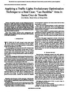
Figure 4: Normalized mutation strength � and normalized progress rate �� as functions of the normalized noise strength � . Note the scaling of the axes. The solid lines represent the values realized by the ����� ��-ES with cumulative step length adaptation and have been obtained from (20) and (21). The dashed lines represent the optimal values obtained by numerically optimizing (6). the dynamics of the process lead to mutation strengths that are too large for normalized noise strengths of up to about � ��� � � � and too small for noise strengths above this value. For zero noise strength, the progress rate that is achieved with cumulative step length adaptation is about 83% of the progress rate that would be achieved with optimally adapted mutation strength. Positive progress rates are achieved up to a normalized noise strength of �� � � � .
�
8
Population Sizing
While sufficient for obtaining a good qualitative understanding of the performance of cumulative step length adaptation in the presence of noise, the approximation considered thus far is too crude for addressing the problem of determining optimal population sizes. From the results obtained so far it appears that by increasing the population size, the strategy can always be made to operate in the regime at the left hand edge of the graphs in Fig. 4 and thus with maximum efficiency. However, it has been seen in [4] that the quality of the approximation given by (5) and (6) deteriorates with increasing population size. In that same reference and in [1], better estimates of the squared length of the progress vector, the signed length of its central component, and the progress rate have been derived. Using those estimates rather than (5) and (6) and not neglecting the �-dependent terms that had been neglected in the derivations of (12) and (20) yields a much improved approximation for the behavior of cumulative step length adaptation. Without going into details, we will present results from that �-dependent analysis here. 14
mutation strength �
20.0
15.0
10.0
5.0
0.0 0.0
5.0
10.0
noise strength
15.0
20.0
15.0
20.0
�
7.0
progress rate ��
6.0 5.0 4.0 3.0 2.0 1.0 0.0 0.0
5.0
10.0
noise strength
�
Figure 5: Normalized mutation strength � and normalized progress rate �� as functions of the normalized noise strength � . The crosses correspond to, from bottom to top, measurements of a ����� ���-ES, a ����� ���-ES, and a ������� ���ES at search space dimensionalities � � �� ��� and � � ��� � �. The solid lines represent the estimates for infinite search space dimensionality given by (20) and (21) that are also depicted in Fig. 4. The dotted lines correspond to the improved approximation that takes some �-dependent terms into account.
�
15
Figure 5 compares the estimates obtained numerically with empirical measurements of the normalized mutation strength and the normalized progress rate of the ����� ��-ES averaged over many time steps on noisy spheres with search space dimensionalities � � �� and � � ���. Also shown are the predictions for infinite � given by (20) and (21). While qualitatively correct, especially the estimates from (21) can be seen to be rather inaccurate even for � as large as ���. The accuracy of the �-dependent estimates is very good in comparison except for high normalized noise strength. In the regime just below � � �� � � � the dynamics of the ����� ��-ES with cumulative step length adaptation are dominated by fluctuations that have been left unconsidered in the present analysis. However, those inaccuracies are tolerable as it will be seen below that the ����� ��-ES optimally uses population sizes large enough to guarantee that the region in which the inaccuracies occur is avoided. The quality of the predictions for the normalized progress rate is not quite as good as for the normalized mutation strength. However, it can also be seen that the inaccuracy of the estimate for the normalized progress rate decreases with increasing � . On the basis of the improved estimates thus obtained, optimal population size parameters and efficiencies can be determined. The efficiency of a strategy is defined in a way that takes not only the progress made but also the computational costs of the optimization into account. Assuming that those costs are dominated by the costs of evaluating the objective function and that other contributions such as those resulting from mutation and recombination can be neglected, the efficiency is commonly defined as the normalized progress rate per evaluation of the objective function, �� �� (22) � Notice that the term � in the denominator is the number of objective function evaluations per time step. Optimal parameter settings can be obtained numerically by optimizing (22). Figure 6 shows the optimal number of offspring per time step � and the maximal efficiency � , i.e. the efficiency for optimally chosen population size parameter settings, as functions of the normalized noise strength � . Also shown are the corresponding values that would be obtained were the mutation strength continually adapted to the optimal values that have been derived in [4]. It can be seen that the efficiencies that cumulative step length adaptation is capable of realizing are — depending on the search space dimensionality and the noise strength — between 15% and 30% below the optimal values. Quite significantly, the right hand graph in Fig. 6 shows that cumulative step length adaptation is robust in the sense that it fails to break down in the presence of noise at least for the range of noise strengths considered. The loss of efficiency that incurs in the presence of noise does not
�
16
0.25
maximal efficiency
opt. number of offspring
150 120 90 60 30 0 0.0
4.0
8.0
12.0
noise strength ���
16.0
0.20 0.15 0.10 0.05 0.00 0.0
4.0
8.0
12.0
noise strength ���
16.0
Figure 6: Optimal number of offspring per time step � and maximal efficiency � as functions of the normalized noise strength � . The curves correspond to, from bottom to top, search space dimensionalities � � ��, � � ���, and � � ����. In the right hand graph, the limiting case � � is included as well. The solid curves depict the results for cumulative step length adaptation. The dotted lines assume optimally adapted mutation strength.
differ qualitatively from that in the absence of noise. As for the population size parameter settings, it can be seen that using cumulative step length adaptation optimal population sizes are below the values computed in [4] for optimally adapted mutation strengths. In the absence of noise, optimal values for � are �, ��, and �� for � � ��, ���, and ����, respectively. In the presence of noise, larger values of � need to be employed in order to achieve optimal efficiency. Overall, it can be said that the choice of a value for � is not very critical provided that � is chosen large enough to support positive progress for the given noise level, and that that choice becomes even less critical with increasing noise strength. For the range of noise strengths and search space dimensionalities considered, optimal values of � are always in the range from � ��� to � ���. Further numerical investigations show that for optimally chosen population size parameters, the strategies always operate in the regime in the left hand half of the graphs in Fig. 4, i.e. that � � � � � � for optimally chosen � and �.
9
Conclusions
What can be learned from the analyses in this paper? It has been seen that the target mutation strength that cumulative step length adaptation seeks to realize is ) in the absence of noise, but generally too optimal (at least in the limit � small in its presence. However, the mutation strength that cumulative step length adaptation actually realizes differs from the target mutation strength as adaptation
�
17
is not instantaneous. The mutation strength that is realized is too large for low noise levels, and too small for high noise levels. The performance loss as compared to optimally adapted mutation strengths has been found to be below 20% in the idealized model from Sect. 7 and below about 30% in the improved model from Sect. 8. In the presence of (not too much) noise, the larger than optimal mutation strengths have the advantage of improving the noise-to-signal ratio that the strategy operates under. Of particular importance to the practitioner is the problem of choosing appropriate settings for the population size parameters. The investigation presented in this paper suggests that between 25% and 30% of the candidate solutions generated should be retained to serve as the population of the next time step. As for choosing how many candidate solutions to generate per time step, higher values buy additional robustness — i.e. the ability to proceed in the presence of higher levels of noise — at the price of decreased efficiency. Cumulative step length adaptation drives the mutation strength to zero if there is too much noise present. A useful course of action is therefore to start out with a relatively small number of candidate solutions to generate per time step, and to gradually increase that number if the strategy is observed to stall. The choice of values for � and � has been found to be rather uncritical. Overall, the performance of the ����� ��-ES with cumulative step length adaptation is robust in that it degrades gradually with increasing noise levels. An empirical evaluation of direct optimization strategies in the presence of noise in [3] has shown that this is not necessarily true for other commonly used approaches, thus making the evolution strategy a promising candidate for the optimization of noisy objective functions.
Acknowledgments This work was supported by the Deutsche Forschungsgemeinschaft (DFG) under grants Be1578/4-2 and Be1578/6-3. The publication of the work was also supported by the DFG as part of the Collaborative Research Center “Computational Intelligence” (SFB 531). Hans-Georg Beyer is a Heisenberg Fellow of the DFG.
References [1] D. V. Arnold, 2001. Local Performance of Evolution Strategies in the Presence of Noise. Dissertation, University of Dortmund, Department of Computer Science. [2] D. V. Arnold and H.-G. Beyer, 2001. “Local performance of the ����� � ��-ES in a noisy environment”. In W. N. Martin and W. M. Spears 18
(eds.), Foundations of Genetic Algorithms 6, pages 127–141. MorganKaufmann Publishers, San Francisco. [3] D. V. Arnold and H.-G. Beyer, 2001. “Noisy optimization with evolution strategies”. Technical Report CI 117/01, SFB 531, University of Dortmund. Available from http://sfbci.informatik.uni-dortmund.de. Submitted for publication. [4] D. V. Arnold and H.-G. Beyer, 2002. “Performance analysis of evolution strategies with multi-recombination in high-dimensional ���-search spaces disturbed by noise”. Theoretical Computer Science. In Press. Available from http://www.sciencedirect.com. [5] T. B¨ack, 1996. Evolutionary Algorithms in Theory and Practice. Oxford University Press, New York. [6] T. B¨ack, D. B. Fogel, and Z. Michalewicz, 1997. Handbook of Evolutionary Computation. Institute of Physics Publishing, Bristol, and Oxford University Press, New York. [7] H.-G. Beyer, 1996. “Toward a theory of evolution strategies: Selfadaptation”. Evolutionary Computation, 3(3):311–347. [8] H.-G. Beyer, 2001. The Theory of Evolution Strategies. Natural Computing Series. Springer Verlag, Berlin. [9] H.-G. Beyer and D. V. Arnold, 2002. “Qualms regarding the optimality of cumulative path length control in CSA/CMA-evolution strategies”. Technical Report CI 129/02, SFB 531, University of Dortmund. Available from http://sfbci.informatik.uni-dortmund.de. Submitted for publication. [10] H.-G. Beyer and K. Deb, 2001. “On self-adaptive features in realparameter evolutionary algorithms”. IEEE Transactions on Evolutionary Computation, 5(3):250–270. [11] A. E. Eiben, R. Hinterding, and Z. Michalewicz, 1999. “Parameter control in evolutionary algorithms”. IEEE Transactions on Evolutionary Computation, 3(2):124–141. [12] P. Gilmore and C. T. Kelley, 1995. “An implicit filtering algorithm for optimization of functions with many local minima”. SIAM Journal on Optimization, 5:269–285.
19
[13] N. Hansen, 1998. Verallgemeinerte individuelle Schrittweitenregelung in der Evolutionsstrategie. Mensch & Buch Verlag, Berlin. [14] N. Hansen and A. Ostermeier, 2001. “Completely derandomized selfadaptation in evolution strategies”. Evolutionary Computation, 9(2): 159– 195. [15] J. Kiefer and J. Wolfowitz, 1952. “Stochastic estimation of a regression function”. Annals of Mathematical Statistics, 23:462–466. [16] S. Kirkpatrick, C. D. Gelatt, and M. P. Vecchi, 1983. “Optimization by simulated annealing”. Science, 220:671–680. [17] T. Lutz and S. Wagner, 1998. “Drag reduction and shape optimization of airship bodies”. Journal of Aircraft, 35(3):345–351. [18] M. Olhofer, T. Arima, T. Sonoda, and B. Sendhoff, 2000. “Optimisation of a stator blade used in a transonic compressor cascade with evolution strategies”. In I. Parmee (ed.), Adaptive Computing in Design and Manufacture, pages 45–54. Springer Verlag, Berlin. [19] J. C. Spall, 2000. “Adaptive stochastic approximation by the simultaneous perturbation method”. IEEE Transactions on Automatic Control, 45(10):1839–1853. [20] J. C. Spall, S. D. Hill, and D. R. Stark, 1999. “Theoretical comparisons of evolutionary computation and other optimization approaches”. Proceedings of the 1999 IEEE Congress on Evolutionary Computation, pages 1398–1405. [21] V. Torczon and M. W. Trosset, 1998. “From evolutionary operation to parallel direct search: Pattern search algorithms for numerical optimization”. Computing Science and Statistics, 29:396–401.
20