Exact and Variational Theorems for Fracture Mechanics of ... - CiteSeerX

International Journal of Fracture, in press, 2000 c 2000 Kluwer Academic Publishers °

Author prepared preprint

Exact and Variational Theorems for Fracture Mechanics of Composites with Residual Stresses, Traction-Loaded Cracks, and Imperfect Interfaces J. A. NAIRN Material Science and Engineering, University of Utah, Salt Lake City, Utah 84112, USA Submitted 8 January 1999

Abstract. By partitioning the total stresses in a damaged composite into either mechanical and residual stresses or into initial and perturbation stresses, it was possible to derive several exact results for the energy release rate due to crack growth. These general results automatically include the effects of residual stresses, traction-loaded cracks, and imperfect interfaces. The exact energy release rate results were expressed in terms of exact solutions to reduced composite stress analysis problems. By considering the common situation where the initial stresses are known exactly, but the perturbation stresses are only known approximately, it was possible to derive rigorous upper and lower bounds to the energy release rate for crack growth. Some of the new fracture mechanics equations were applied to crack closure calculations, to fiber fracture and interfacial debonding in the fragmentation test, and to microcracking in composite laminates. 1.

Introduction

Composite materials, especially composites reinforced with aligned, high-modulus fibers, are often very close to being linear elastic up to failure. For this reason, many composite fracture models for composites have been developed using linear-elastic fracture mechanics [1, 2]. There is microscopy evidence of large amounts of matrix deformation on fracture surfaces [3], but the fact that this deformation does not lead to non-linear, load-deformation curves suggests it is not a major factor in the global energy released during crack growth. The matrix deformation may play a role in toughness [3], but it should be possible to calculate the energy release rate due to crack growth by ignoring such deformation and then assuming that cracks propagate when that energy release rate exceeds the fracture toughness of the composite. The required energy release rate can be calculated from a global energy balance using G=−

d(W − U ) dΠ = dA dA

(1)

where Π is thermoelastic potential energy, W is external work, U is thermoelastic internal energy, and dA is an increment in total crack area. [4]. The required terms can be calculated using linear thermoelasticity methods. The goal of this paper is to apply (1) to general composite fracture problems when the composite is assumed to be a linear elastic material. Despite the simplification of linear elasticity, there are several added complexities in heterogeneous composites materials that make fracture mechanics of composite materials more difficult that the corresponding analysis for homogeneous materials. First, because composites are comprised of materials with disparate thermal expansion coefficients, the phases will inevitably be subjected to residual stresses [5]. These residual stresses can contribute to energy release rate and should be part of every composite fracture model [6]. Second, the heterogeneity of composites sometimes causes cracks to divert in directions that would not be observed in homogeneous materials. If such structure-controlled crack growth results in crack surfaces that contact each other, there may be crack surface tractions. When traction-loaded crack surfaces slide relative to each other during crack growth, that sliding can affect the energy release rate. Third, there will always be interfaces between phases. If these interfaces are not perfect, they may slide relative to each other during crack growth [7]. Like sliding traction-loaded cracks, sliding imperfect interfaces can affect the energy release rate. The main results of this paper are to apply (1) to general composite fracture problems and derive several new and exact results for energy release rate. All new results include the effects of residual stresses, traction-loaded crack surfaces, and imperfect interfaces. 1

J. A. Nairn

2

The fracture mechanics results for composites are derived in the section on Fracture Mechanics Theorems. The basic method was to partition the total stresses into residual and mechanical stresses or into initial and perturbation stresses. Then, by various applications of virtual work theorems and the divergence theorem it was possible to express (1) in several alternate forms that are more convenient for analysis of particular composite fracture problems. A total-stress form was derived by recombining either of the partitioned-stress results. All new equations are exact but were expressed in terms of exact solutions to composite stress analysis problems that typically will not have exact solutions. A previous paper [6] derived related exact expressions but only considered residual and mechanical stress partitioning and traction-free cracks; this paper extends that work to include traction-loaded cracks and imperfect interfaces and to additionally consider initial and perturbation stress partitioning. By partitioning the total stresses into exact initial stresses and approximate perturbation stresses, it was possible to recast the exact results as rigorous bounds to the energy release rate rate for crack growth. It is shown how these bounds can be applied to finite fracture mechanics analysis of composite fracture events. A previous paper [8] derived a rigorous upper bound to the finite energy release rate when there are traction-free cracks; this paper extends that work to include both upper and lower bounds, to derive bounds for both infinitesimal and finite fracture events, and to include the effects of traction-loaded cracks and imperfect interfaces. The Examples section shows how the new results can be applied to crack closure calculations, to fiber fracture and interfacial debonding in the fragmentation test, and to microcracking in composite laminates. 2.

Fracture Mechanics Theorems

Consider an arbitrary composite subjected to a uniform temperature change of ∆T = T and to any mixed traction and displacement boundary conditions as illustrated in Fig. 1. Let the boundary be S = ST ∪ Su , where ST is that part of the surface subjected to traction boundary conditions and Su is that part of the surface subjected to displacement boundary conditions. Let σ, with associated tractions on the boundary of T~ = σ n ˆ where n ˆ is a unit normal to the surface, and ε, with associated displacements ~u , be the exact solution to the linear thermoelasticity problem σn ˆ = T~ 0

on

ST

~u = ~u 0

on

Su

σ = C(ε − αT )

and

ε = Sσ + αT

(2)

where, in addition, σ satisfies equilibrium and ε and ~u satisfy strain-displacement relations. The terms C, S, and α are the stiffness, compliance, and thermal expansion tensors; in composites these material properties will depend on position. For arbitrary problems, the traction T~ 0 , and displacement, ~u 0 , boundary conditions may also depend on position. Note also that tractions and displacements may be applied over the same portions of the surface provided they are applied along orthogonal directions. Let the interior of the composite contain cracks and interfaces and denote the total surface area of cracks and interfaces as Sc . Across any crack or interface, static equilibrium requires that stresses be continuous, but displacements may be discontinuous. When cracks open, the surfaces will be traction free which corresponds to continuous zero stresses. The displacements, however, may be discontinuous as the two surfaces displace independently. When cracks close there may be contact compressive or shear stresses. These stress will be continuous but displacements may be discontinuous as the crack surfaces slide relative to each other. Interfaces may be perfect or imperfect. At perfect interfaces, stresses and displacement are continuous. Imperfect interfaces can be modeled by requiring continuous stresses, but allowing displacements to be discontinuous [7]. Thus opened cracks, closed cracks, perfect interfaces, and imperfect interfaces can all be included in the single interior surface Sc with continuous stresses but possibly discontinuous displacements. An additional boundary condition on Sc is T~ = T~c

on Sc

(3)

where T~c includes traction loads on any cracks or tractions induced at sliding interfaces. In general, T~c may depend on position.

3

,, ,,,, ,,, ,,

Exact and Variational Fracture Mechanics Theorems

ST →

→ 0

T=T

Su →

→

u = u0 σ = C( ε − αT)

Sc

→

ε = Sσ + αT →

T = T0

→

→ 0

u=u

ST

Su

Fig. 1. An arbitrary multiphase material subjected to traction and displacement boundary conditions and containing cracks and interfaces.

The goal of this section is derive exact and variational theorems for the energy release rate due to an increase in total crack area for the arbitrary composite in Fig. 1. An increase in crack area corresponds to an increase in the internal area Sc . 2.1.

Mechanical and Residual Stresses

The full thermal elasticity problem can be treated as a superposition of two problems. First, let σ m and εm , with tractions T~ m and displacements ~u m , be the exact solution to the isothermal (T = 0) elasticity problem: ˆ = T~ 0 on ST , ~u m = ~u 0 on Su , σ m = Cεm , and εm = Sσ m (4) σm n Second, let σ r and εr , with tractions T~ r and displacements ~u r , be the exact solution to the thermal elasticity problem: ˆ = 0 on ST , σr n

~u r = 0 on Su ,

σ r = C(εr − αT ),

and εr = Sσ r + αT

(5)

A superposition of the above two solutions, σ = σ m + σ r and ε = εm + εr , exactly solves the complete thermal elasticity problem in (2) and (3) provided T~ m + T~ r = T~c

on Sc

(6)

σ m and εm are the mechanical stresses and strains while σ r and εr are the residual thermal stresses and strains. By substituting the partitioned stresses into (1) and making use of virtual work and divergence theorems (the details are in the Appendix), it is possible to derive the first energy release rate theorem: µ ¶ µZ ¶ Z d hσ m · αi d hσ r · αi d VT 1 2 + + T~ r · ~u m dS + T~ r · ~u r dS (7) G = Gmech + 2 dA dA dA 2 Sc Sc where Gmech is the mechanical energy release rate or the energy release when T = 0: ¶ µ Z Z Z d 1 1 1 0 m m 0 m m ~ ~ ~ T · ~u dS − T · ~u dS + T · ~u dS Gmech = dA 2 ST 2 Su 2 Sc and angle brackets indicates a volume-averaged quantity: Z 1 f (x, y, z)dV hf (x, y, z)i = V V

(8)

(9)

J. A. Nairn

4

Equation (7) is exact. The first term is the traditional energy release rate. The subsequent terms are required in many composite fracture problems to account for effects of residual stresses, traction-loaded cracks, and imperfect interfaces. A similar analysis for traction-free cracks and perfect interfaces is given in Ref. [6]. The new terms above involving integrals over Sc extend those results to include traction-loaded cracks and imperfect interfaces. In Ref. [6], it was argued that during pure mode I crack growth (or similarly during pure mode II or mode III crack growth) the mode I energy release rate must scale with mode I stress intensity factor squared, KI2 . Furthermore, for linear elastic materials in which all applied tractions and displacements are scaled by a factor P and the temperature difference T is scaled by a factor T ∗ , KI must scale by a linear combination of P and T ∗ . Thus GI ∝ KI2 = (c1 P + c2 T ∗ )2

(10)

Comparing (10) to (7) similarly scaled by P and T ∗ , we can prove that V T d hσ m · αi 1 d + 2 dA 2 dA Gmech

Z T~ r · ~u m dS Sc

Z V T d hσ r · αi 1 d + T~ r · ~u r dS 2 dA 2 dA Sc Z = V T d hσ m · αi 1 d + T~ r · ~u m dS 2 dA 2 dA Sc

(11)

Substitution into (7) gives the pure mode I energy release rate of 

GI Gmech

V T d hσ m · αi 1 d +  2 dA 2 dA  = 1 + Gmech

Z T~ r · ~u m dS Sc

2   

(12)

This result extends the analogous result in Ref. [6] to include traction-loaded cracks and imperfect interfaces. 2.2.

Total Stresses

Sometimes it is simpler to have an energy release rate result in terms of total stresses instead of partitioned stresses. By comparing the two virtual work results in the Appendix in (87) and (88) we quickly derive Z

Z

Z

Z

T~ 0 · ~u r dS −

σ m · αT dV = V

T~ r · ~u 0 dS +

ST

Su

Z T~ m · ~u r dS −

Sc

T~ r · ~u m dS

(13)

Sc

Substituting half of (13) for half of the hσ m · αi term in (7) leads to an second energy release rate theorem, now in terms of total stresses (σ), tractions (T~ ), and displacements (~u ): G=

1 d 2 dA

µZ

Z T~ 0 · ~u dS −

ST

Su

T~ · ~u dS + Sc

¶

Z

Z T~ · ~u 0 dS +

σ · αT dV

(14)

V

For the special case of traction-only boundary conditions, (14) followed by use of the divergence theorem leads to ¶ µZ Z Z ¢ ¡1 d 1 d 0 ~ σ · αT dV = σSσ + σ · αT dV (15) T · ~u dS + G= 2 dA dA V 2 S+Sc V This result is identical to the thermoelastic fracture mechanics result derived by Hashin [8]. In other words, (14) extends Hashin’s analysis (i.e. (15)) to include mixed boundary conditions. Note also that the integrand in (15) is minus the Gibb’s free energy, F (written as F here to avoid confusion with energy release rate G), less entropy or heat capacity terms [9–11]. Because the constant heat-capacity terms drop out when evaluating the derivative with respect to crack area for an elastic material, (15) shows that energy release rate is equal to a Gibb’s free energy derivative, G = −dF/dA, when there are traction-only boundary conditions.

5

2.3.


Initial and Perturbation Stresses

To derive some alternative fracture mechanics theorems, including results that help derive a variational fracture mechanics theorem, we consider a different stress partitioning scheme. The full thermal elasticity problem can alternatively be partitioned into initial and perturbation stresses. First, let σ 0 and ε0 , with tractions T~ 0 and displacements ~u 0 , be the exact solution to the thermal elasticity problem: ¡ ¢ ˆ = T~ 0 on ST , ~u = ~u 0 on Su , σ 0 = C ε0 − αT , and ε0 = Sσ 0 + αT (16) σ0 n for any composite which may have cracks and imperfect interfaces on an initial surface Sc0 . Now let Sc0 expand into a larger crack and imperfect surface area, Sc , and, let σ p and εp , with tractions T~ p and displacements ~u p , be the exact solution to the isothermal (T = 0) elasticity problem: T~ p = 0 on ST ,

~u p = 0 on Su ,

T~ p = T~c − T~c0 on Sc ,

σ p = Cεp

and εp = Sσ p

(17)

where T~c0 is the initial stress state traction at the locations of the cracks and interfaces on Sc . Note that T~ p may be nonzero on Su and ~u p may be nonzero on ST and Sc . A superposition of the above two solutions, σ = σ 0 + σ p and ε = ε0 + εp , exactly solves the complete thermal elasticity problem in (2) and (3). σ 0 and ε0 are the initial stresses and strains; σ p and εp are the perturbation stresses and strains or the change in stresses and strains due to growth of traction-loaded cracks and sliding of imperfect interfaces. By substituting initial and perturbation stresses into (1) and making use of virtual work and divergence theorems (the details are in the Appendix), it is possible to derive a third energy release rate theorem expressed three different ways: µZ ¶ Z 1 d p 0 p p ~ ~ T · ~u dS + T · ~u dS G = dA 2 Sc S µZ c µZ ¶ ¶ Z Z 1 d 1 d p 0 p p p 0 p p ~ ~ T · ~u dS + T · ~u dS + σ Sσ dV = ε Cε dV (18) = dA 2 V dA 2 V Sc Sc In many problems it may be convenient to take the initial state as the undamaged composite with perfect interfaces and the perturbation stresses as the change in stresses due to introduction of cracks and imperfect interfaces. In an undamaged composite ~u 0 must be continuous across all cracks and interfaces. Because the area Sc has two sides and the traction vector T~ p changes sign from one side to the other, when ~u 0 is continuous, the first integral in each form of (18) vanishes giving the special case result of ¶ ¶ ¶ µ Z µ Z µ Z d d 1 1 1 d σ p Sσ p dV dV = εp Cεp dV dV (19) T~ p · ~u p dS = G= dA 2 Sc dA 2 V dA 2 V In other words, the total energy release rate including residual stresses, traction-loaded cracks, and imperfect interfaces, can be evaluated by finding the change in perturbation stress energy due to formation of damage. Notice that the perturbation stress analysis is an isothermal (T = 0) stress analysis. Thus the effect of thermal stresses on the energy release rate can be evaluated here completely by a thermoelasticity analysis of the undamaged composite only; there is never a need to conduct a thermoelasticity analysis of a cracked body. If we partition the total stresses in (14) into initial and perturbation stresses and delete derivatives of the constant initial stresses, we get µZ ¶ Z Z Z Z 1 d 0 p p 0 0 p p ~ ~ ~ ~ σ · αT dV (20) T · ~u dS − T · ~u dS + Tc · ~u dS + Tc · ~u dS + G= 2 dA ST Su Sc Sc V This result appears different than (18), but can be shown to be identical. Equating the two virtual work results between initial and perturbation stresses in the Appendix in (93) and (95), gives Z Z Z Z Z σ p · αT dV = (21) T~ p · ~u 0 dS + T~ p · ~u 0 dS − T~ 0 · ~u p dS − T~c0 · ~u p dS V

Su

Sc

ST

Substitution of (21) into (20) and subtracting zero in the form µZ ¶ 1 d 0 0 ~ Tc · ~u =0 2 dA Sc leads to a result that is identical to (18).

Sc

(22)

J. A. Nairn

2.4.

6

Generalized “Levin” Relations

In a pioneering composite mechanics paper, Levin considered an undamaged composite with traction loading and perfect interfaces [12]. By partitioning the stresses into mechanical and residual stresses and making use of two applications of virtual work, he derived (in the nomenclature of this paper): Z Z m T~ 0 · ~u r dS σ · αT dV = (23) V

ST

Levin’s result is a special case of (13); in other words, (13) generalizes Levin’s equation to account for mixed boundary conditions, traction-loaded cracks, and imperfect interfaces. Similarly, (21) was derived by two applications of virtual work between partitioned initial and perturbation stresses; it can therefore be considered as a new, generalized, Levin-type relation. In Ref. [12], Levin derived a powerful application of (23) for determining the effective thermal expansion coefficients of a composite from a solution for the mechanical-only stresses in that composite. Here (13) had an important use in deriving the total stress result in (14) from the partitioned mechanical and residual stress result in (7). Similarly, (21) was needed to show the identity between the total stress result in (14) and the perturbation stress result in (18). 2.5.

Variational Theorems

All results in the previous sections are exact, but they are written in terms of exact solutions to composite stresses and strains. In general, such exact solutions will not be known. In this section, we again partition the stresses into initial and perturbation stresses. We assume that the initial stresses are known exactly. We assume that the perturbation stresses and strains result from the formation of a new finite amount a fracture area, ∆A, and that the perturbation stress state is only known approximately. The goal is to find rigorous upper and lower bounds to the total energy release rate, ∆G, due to the fracture event of forming the finite amount of crack area. First consider an approximate perturbation solution written in terms of an admissible stress state, σ pa . To be an valid admissible stress state, σ pa must satisfy equilibrium and tractions associated with σ pa must give the proper boundary conditions on both ST and Sc . The thermoelastic complementary energy associated with this approximate stress state is [13] Z Z Z ¡ 0 ¢ 1 0 p 0 p 0 p (σ + σ a )S(σ + σ a )dV + (σ + σ a ) · αT dV − (24) T~ + T~ap · ~u 0 dS Γa = 2 V V Su Substituting the virtual work result in the Appendix in (95) (which is valid for any admissible stress state), the approximate complementary energy of the composite reduces to Z Z 1 p 0 ~ σ p Sσ pa dV (25) Ta · ~u dS + Γa = Γ0 + 2 V a Sc where Γ0 =

1 2

Z

Z

V

Z T~ 0 · ~u 0 dS

σ 0 · αT dV −

σ 0 Sσ 0 dV + V

(26)

Su

is the exact complementary energy of the initial stresses. By the principle of minimum complementary energy, this approximate result must be greater than the true complementary energy. Defining the true complementary energy from the exact perturbation stresses, σ p , and tractions, T~ p , we have Z Z Z Z 1 1 p 0 p p p 0 ~ ~ σ Sσ dV ≤ Γ0 + σ p Sσ pa dV (27) T · ~u dS + Ta · ~u dS + Γ0 + 2 V 2 V a Sc Sc By a discrete evaluation of the derivative in (18) for the formation of finite fracture area ∆A causing the stresses to change from σ 0 to σ 0 + σ p followed by a comparison to (27), the energy release rate for the process is seen to be bounded from above by: µZ ¶ Z 1 1 T~ap · ~u 0 dS + σ pa Sσ pa dV (28) ∆G ≤ ∆A 2 V Sc

7


If the initial stresses correspond to an undamaged composite with continuous ~u 0 on Sc , the first term vanishes and the upper bound to ∆G is given simply by the stress energy of any admissible perturbation stress state. Hashin previously considered an undamaged initial state, traction-free crack surfaces, and mechanical-only stresses and derived a result identical to (25) [14] but did not have the Sc integral because of the undamaged initial state. Hashin later added residual stresses and derived an upper bound result equivalent to (28) but again lacking the Sc integral [8]. Although Hashin’s two analyses used more restrictive assumptions then used here, both his results are all seen to be correct in general for any undamaged initial state, even when there are mixed boundary conditions, traction-loaded cracks, and imperfect interfaces. The new integral over Sc in (28) extends Hashin’s results to the case where the initial stress state is for a damaged composite. For a lower bound to ∆G, we consider approximate solutions based on admissible strain states, εpa , and the approximate change in potential energy. To be a valid admissible strain state, εpa must be derived from an assumed displacement field, ~uap , which gives the proper boundary conditions on Su . If the exact, initial stresses have a potential energy Π0 , the introduction of new damage will cause the potential energy to decrease by an amount ∆Π = −∆G∆A. For any admissible strain state, the approximate potential energy must be greater than the true potential energy. Thus trivially, an approximate change in potential energy, ∆Πa , provides a lower bound to ∆G: ∆Πa (29) ∆G ≥ − ∆A The only work that remains is to express ∆Πa in a convenient form using the admissible strain state. The thermoelastic potential energy associated with an approximate, admissible strain state is not given by (98) in the Appendix because that result used (96) which is not valid for general admissible strain states. All other steps used to derive (98), however, are valid for any admissible strain state. Thus, if we eliminate the final use of (96) and use the crack surface boundary conditions, the approximate thermoelastic potential energy can be written as Z Z Z ¡ ¢ 0 ¡ ¢ p 1 0 0 ~ ~ ~ ~ εp Cεp dV (30) Tc − Tc · ~u dS − Tc − Tc · ~ua dS + Πa = Π0 − 2 V a a Sc Sc The lower bound to ∆G becomes ¶ µZ Z Z ¡ ¢ ¡ ¢ 1 1 εpa Cεpa dV T~c − T~c0 · ~u 0 dS + T~c − T~c0 · ~uap dS − ∆G ≥ ∆A 2 V Sc Sc

(31)

Again, the first integral vanishes if the initial strain state corresponds to an undamaged composite with ~u 0 continuous on Sc . We can define the approximate changes in complementary and potential energy due to any admissible stress or strain states, respectively as Z Z 1 T~ap · ~u 0 dS σ pa Sσ pa dV + (32) ∆Γa = 2 V Sc Z Z Z ¡ ¢ ¡ ¢ 1 εpa Cεpa dV − (33) T~c − T~c0 · ~u 0 dS − T~c − T~c0 · ~uap dS ∆Πa = 2 V Sc Sc By (28) and (31), the rigorous bounds on the energy release rate due the formation of a finite amount of fracture area are ∆Γa ∆Πa ≤ ∆G ≤ (34) − ∆A ∆A The most common application of these rigorous bounds to composite energy release rate will probably be for the initiation of damage. It will often be possible to derive exact (or essentially exact) results for the stresses in the undamaged composites. The bounds on energy release rate can then be derived from any approximate solutions for the stresses in the cracked composite. In many composite failure analyses, however, the concern is not just with the initiation of damage, but also with the subsequent propagation of damage. If we introduce fracture area as a variable, the total energy release rate due to a fracture event extending damage area from A1 to A2 can be written exactly in terms of energy release rates for forming fracture area A1 or A2 from the initial undamaged composite: ∆G(A1 → A2 ) =

A2 ∆G(0 → A2 ) − A1 ∆G(0 → A1 ) A2 − A1

(35)

J. A. Nairn

8

By making use of the rigorous bounds on ∆G for damage initiation, it is possible to rigorously bound the damage propagation energy release rate by −

∆Γa (0 → A2 ) + ∆Πa (0 → A1 ) ∆Πa (0 → A2 ) + ∆Γa (0 → A1 ) ≤ ∆G(A1 → A2 ) ≤ A2 − A1 A2 − A1

(36)

Unless the rigorous bounds for damage initiation (from (34)) are very tight, the rigorous bounds for damage propagation (from (36)) are likely to be far apart. Perhaps the rigorous propagation bounds are too pessimistic. Because the admissible stress or strain states each provide approximate solutions, we could continue and define approximate energy release rates derived from each approximate solution using ∆G1 (A1 → A2 ) ∆G2 (A1 → A2 )

∆Γa (0 → A2 ) − ∆Γa (0 → A1 ) A2 − A1 ∆Πa (0 → A2 ) − ∆Πa (0 → A1 ) = − A2 − A1 =

(37) (38)

∆G1 (A1 → A2 ) and ∆G2 (A1 → A2 ) will, in general, be much closer to each other than the bounds in (36). Perhaps, therefore, in practice, they will provide tighter, albeit non-rigorous, bounds to ∆G(A1 → A2 ). An example of using such practical bounds to analyze composite microcracking will be given in the Examples section. 2.6.

Finite Fracture Mechanics

The previous section dealt with a finite amount of fracture growth — ∆A. Traditional fracture mechanics, however, deals with an infinitesimal amount of crack propagation. Such mathematical results can be derived from finite fracture results by taking the limit as ∆A → 0, but that limit may not always be appropriate. Many composite failures do not proceed by infinitesimal crack growth, but rather proceed by discrete fracture events [8]. Two examples are fiber fracture events [15] and matrix microcracking events [2]. Associated with any fracture event is a finite amount of new fracture area, ∆A. One could claim that fracture mechanics can not handle fracture events, or one could propose that the fracture event occurs when the total energy release rate for that fracture event, ∆G, exceeds the material toughness for that event. The method of predicting fracture events based on event energy release rate has been used for many composite failure problems such as edge delamination [16], matrix microcracking [2], fiber breakage and interfacial debonding [17], and cracking of coatings [18–20]. Hashin has recently proposed calling this approach to fracture mechanics finite fracture mechanics [8]. The results in the previous section provide variational analysis tools for evaluating energy release rate for fracture events. Two examples in the following section give applications of finite fracture mechanics to predicting composite failure. 3.

Examples

The five key energy release rate results are in (7), (14), (18), (34), and (36). Some applications using the mechanical and residual stress partitioning of (7) are given in Ref. [6]. An analysis using the total stress form of (14) including a traction-loaded crack is given in Ref. [21]. This section will give some examples of partitioning into initial and perturbation stresses and using (18), (34), and (36). 3.1.

Crack Closure in Finite Element Analysis

Consider a small amount of crack growth caused by opening the grid between two elements causing new crack surface area ∆A. The initial stresses are taken to be the stresses before the new crack area forms; the perturbation stresses are the change in stresses caused by the new crack growth or by opening the area between two elements. Evaluation of the derivative in (18) by taking the limit as ∆A → 0 results in µZ ¶ Z 1 1 T~ p · ~u 0 dS + T~ p · ~u p dS (39) G = lim ∆A→0 ∆A 2 Sc Sc

9


Notice that these integrals extend over the entire crack and interface surfaces in Sc . Most crack closure methods only consider the work required to close the new crack area and thus only integrate over the area S = ∆A local to the crack tip [22]. The result in (39) shows that such crack closure calculations are invalid when there are variable tractions along crack surfaces or slippage at imperfect interfaces. A good example of variable crack surface tractions is friction modeled by having the crack surface shear stress, τ , being related to the crack surface normal stress, σn , through a friction law τ = µσn where µ is the coefficient of friction. When a friction-loaded crack is extended by a finite amount ∆A, σn may change along the entire crack surface and thus the crack closure integral must consider all of Sc and not just the new crack area of S = ∆A. The condition for local crack-tip crack-closure calculations to be valid are that T~ p must be zero except on the area S = ∆A. These conditions are satisfied when all interfaces are perfect and when all crack surfaces are traction free. Under such conditions, (39) reduces to Z ¡ ¢ 1 −T~c0 · ~u p dS (40) G = lim ∆A→0 2∆A S=∆A which reduces to a standard crack closure integral when account is made for integration over both surfaces of the new crack area [22]. Local crack closure is also valid in the presence of crack surface tractions, provided there is no change in crack surface tractions along the original crack surfaces. For this situation, T~ p will be zero every place except on S = ∆A near the crack tip. Such tractions are included in (40) be replacing −T~c0 with T~c − T~c0 where T~c is the constant crack surface traction. 3.2.

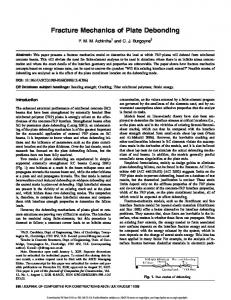
Fragmentation Test

In the fragmentation test [15], a single fiber is embedded in a large amount of matrix and the specimen is loaded in tension until the fiber fragments. On continued loading the fiber continues to fragment eventually forming a roughly periodic array of fiber fragments. To analyze a fragmentation specimen, we consider a unit cell of damage or a single fiber fragment as illustrated in Fig. 2. The fiber fragment is of length l and radius rf ; the matrix is assumed to be infinite. The stresses are partitioned into initial and perturbation stresses. The initial stresses can easily be found by an exact analysis to two concentric cylinders with a perfect interface (Fig. 2B); such a solution is given in Ref. [23]. The boundary conditions for normalized perturbation stresses are zero displacement on the matrix ends and −1 compression on the fiber ends (Fig. 2C). The full perturbation stresses are obtained by multiplying the normalized result by ψ∞ where ψ∞ is the initial axial stress in the fiber and is given in Ref. [23]; superscript p in this section indicates normalized perturbation stresses and displacements. We can analyze the fragmentation specimen using (18). The crack and interface surfaces, Sc , include the two fiber breaks and the matrix and fiber surfaces along the interface at r = rf . The fiber fracture surfaces are traction free; thus on the two fiber ends 2 wfp (±l/2, r) (T~c − T~c0 ) · ψ∞ ~u p = ∓ψ∞

(41)

On the fiber/matrix interfacial surfaces: Fiber Surface : Matrix Surface :

i h 2 p p (z, rf )wfp (z, rf ) + (σrr (z, rf ) − σ ∗ )upf (z, rf ) τrz (T~c − T~c0 ) · ψ∞ ~u p = ψ∞

(42)

2 p p p [τrz (z, rf )wm (z, rf ) + (σrr (z, rf ) − σ ∗ )upm (z, rf )] (43) (T~c − T~c0 ) · ψ∞ ~u p = −ψ∞

p (z, r) are the perturbation axial displacements of the fiber and matrix, upf (z, r) and where wfp (z, r) and wm p p p (z, rf ) and σrr (z, rf ) are the um (z, r) are the perturbation radial displacements of the fiber and matrix, τrz ∗ perturbation interfacial stresses, and ψ∞ σ is the interfacial radial stress in the initial stresses [23]. Notice p is zero due to axisymmetry and thus there is no term from the hoop displacements. Substitution of that τrθ the Sc conditions into (18) and assuming symmetry about z = 0 gives " # Z l/2 D E d p 2 p r2 wf (l/2) + rf τrz (z, rf )[wp ]dz (44) G = −πψ∞ dA f −l/2

J. A. Nairn

σ0 τrz=0 w2=con.

τrz=0 w2= -con.

,,,,,,, ,,,,,,, ,,,,,,, ,,,,,,, ,,,,,,, ,,,,,,, ,,,,,,, ,,,,,,, ,,,,,,, ,,,,,,, ,,,,,,, ,,,,,,, ,,,,,,, ,,,,,,, ,,,,,,, ,,,,,,, ,,,,,,, ,,,,,,, ,,,,,,, ,,,,,,, ,,,,,,, ,,,,,,, ,,,,,,, ,,,,,,, ,,,,,,, ,,,,,,, ,,,,,,, ,,,,,,, ,,,,,,, ,,,,,,, ,,,,,,, ,,,,,,, ,,,,,,, ,,,,,,, ,,,,,,, ,,,,,,, ,,,,,,, ,,,,,,, ,,,,,,, ,,,,,,, ,,,,,,, ,,,,,,, ,,,,,,, ,,,,,,, ,,,,,,, ,,,,,,, ,,,,,,, ,,,,,,,

σ0 τrz=0 w=con.

ld/2

τrz=0 w= -con.

−ψ∞

σ0

,,,,,,, ,,,,,,, ,,,,,,, ,,,,,,, ,,,,,,, ,,,,,,, ,,,,,,, ,,,,,,, ,,,,,,, ,,,,,,, ,,,,,,, ,,,,,,, ,,,,,,, ,,,,,,, ,,,,,,, ,,,,,,, ,,,,,,, ,,,,,,, ,,,,,,, ,,,,,,, ,,,,,,, ,,,,,,, ,,,,,,, ,,,,,,, ,,,,,,, ,,,,,,, ,,,,,,, ,,,,,,, ,,,,,,, ,,,,,,, ,,,,,,, ,,,,,,, ,,,,,,, ,,,,,,, ,,,,,,, ,,,,,,, ,,,,,,, ,,,,,,, ,,,,,,, ,,,,,,, ,,,,,,, ,,,,,,, ,,,,,,, ,,,,,,, ,,,,,,, ,,,,,,, ,,,,,,, ,,,,,,,

=

τrz=0 w2=0

+ τrz=0 w2=0

σ0

σ0 ψ∞ ∆Τ=Τ

σ0 ∆Τ=Τ A. Total Stresses

ψ∞

10

B. Initial Stresses

,,,,,, ,,,,,, ,,,,,, ,,,,,, ,,,,,, ,,,,,, ,,,,,, ,,,,,, ,,,,,, ,,,,,, ,,,,,, ,,,,,, ,,,,,, ,,,,,, ,,,,,, ,,,,,, ,,,,,, ,,,,,, ,,,,,, ,,,,,, ,,,,,, ,,,,,, ,,,,,, ,,,,,, ,,,,,, ,,,,,, ,,,,,, ,,,,,, ,,,,,, ,,,,,, ,,,,,, ,,,,,, ,,,,,, ,,,,,, ,,,,,, ,,,,,, ,,,,,, ,,,,,, ,,,,,, ,,,,,, ,,,,,, ,,,,,, ,,,,,, ,,,,,, ,,,,,, ,,,,,, ,,,,,,

ld/2

−ψ ∞ ∆Τ=0 C. Perturbation Stresses

Fig. 2. The analysis of a single fiber fragment (A) can be partitioned into the initial stresses (B) and the perturbation stresses (C). The initial stresses are the stresses for an infinitely long, unbroken fiber in an infinite matrix under an applied stress of σ0 and temperature differential of T . The perturbation stresses are the stresses for a fiber fragment loaded by compression stress of ψ∞ while the matrix ends are maintained at zero displacement. The notation “con.” means a constant that is independent of r.

D Here

E p wfp (l/2) is the average axial perturbation displacement on the fiber end and [wp ] = wm (z, rf ) −

wfp (z, rf ) is the axial displacement discontinuity at the fiber/matrix interface. There is also a term involving radial displacement discontinuity, [up ], but because the radial stresses are predominantly compressive, it has been argued that the radial displacement discontinuity is zero even in the presence of an imperfect interface [17, 23]; it was assumed to be zero for the derivation of (44). Two previous papers [17, 23] considered the energetics of the fragmentation specimen. After conversion of the dimensionless results in those papers to the dimensioned results used here, there is found to be a difference between (44) and the previous results. The difference is a change of sign on the second term in (44) or the integral along the interface. The previous papers argued that because of the infinite matrix, there is no external work and G reduces to G = −dU/dA. That argument was wrong. When there are traction-loaded cracks or imperfect interfaces, there is the potential for external work along Sc . The general theory in this paper includes all external work and thus (44) corrects the errors in Refs. [17] and [23]. Fortunately, the correction only affects the magnitude of some previous results and does not alter any conclusions. Additionally, for the case of perfect interfaces and traction-free cracks, the second term in (44) vanishes and the results in Refs. [17] and [23] are correct. 3.3.

Fiber Breakage with an Imperfect Interface

Hashin has proposed a simple imperfect interface model where the displacement discontinuity is linearly related to the associated stress at the interface [7] which for the fragmentation test reduces to [wp ] =

p (rf ) τrz Ds

(45)

where Ds is a property of the interface or interphase. Ds → ∞ corresponds to a perfect interface; any other Ds describes an imperfect interface with Ds → 0 corresponding to a traction-free debonded interface. Substitution in (44) and evaluating the discrete derivative for the fiber fragment of length l breaking into two fragments of length l/2 with dA = πrf2 , the total energy release rate for fiber fracture is ¡ ¢ 2 2H(l/2) − H(l) ∆Gf = ψ∞

(46)

11


1.2 ds = 300 MPa

1.0

d s = 1000 MPa

Gf (mJ/m2)

0.8 0.6

ds = ∞

0.4 0.2 0.0 0

1

2

3 4 5 Crack Density (1/mm)

6

7

8

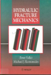
Fig. 3. Energy release rate for a fiber fracture event as a function of the crack density of fiber breaks for various values of the interface parameter, ds . These calculations were for a glass fiber (Ef = 72 GPa, vf = 0.20, and rf = 7.5 µm ) in a polymeric matrix (Em = 1.68 GPa, vm = 0.355) and an applied axial load adjusted to have ψ∞ = 1.

where after defining a new interface parameter ds = rf Ds H(l) = −

D

E

wfp (l/2)

1 − ds

Z

l/2

−l/2

2

p (τrz (rf )) dz

(47)

Sample calculations for ∆Gf as a function of fragment length (1/crack density) for glass fibers in a polymeric matrix and various values of the interface parameter are given in Fig. 3. The required perturbation p (rf ) for these calculations were found using the Bessel-Fourier stress function analysis terms wfp (l/2) and τrz derived in Ref. [23]. This plot corrects the similar plot in figure 2 of Ref. [17] for the sign error in the imperfect interface term in H(l). The corrected sign error causes the changes for a specific ds vs. ds = ∞ to now be smaller; all trends of the curves, however, are the same and the results with a perfect interface (ds = ∞) are identical. A detailed discussion of ∆Gf is given in Ref. [17]. In brief, the energy release rate for the first fiber breaks (at low crack density) gets higher as the interface gets more imperfect. An imperfect interface allows interfacial slip after the fiber break which releases more energy than when slip is prevented by a perfect interface. 3.4.

Fiber/Matrix Debonding with Friction

For a debonding analysis, debond zones of length ld /2 are added to each end of the fragment (see Fig. 2). When there are friction effects, the debonds will be loaded by shear traction. By Coulomb friction, the friction shear-stress should be τrz (z, rf ) = ±µσrr (z, rf ) where µ is the coefficient of friction of the fiber/matrix interface and the sign is adjusted depending on the sliding direction. In an exact friction model, one must account for variations in σrr (z, rf ) along the debond; for a simpler model, we assume the friction stresses are constant and given by τf = ±µ hσrr (rf )i where hσrr (rf )i is the average interfacial normal stress in the debond zone. The average normal stress must be linearly related to the applied load (ψ∞ ). Thus we can write the frictional stresses as τf = ±ψf ψ∞ where ψf is an effective coefficient of friction. The correct signs for τf are to be negative in the debond zone at z = −l/2 and positive in the debond zone at z = l/2. Finally, because the above fragmentation analysis used normalized perturbation stresses, the normalized shear stress p (z, rf ) = ±ψf . in the debond zone of this friction model are τrz For simplicity, we assume symmetric debonding damage and a perfect interface in the bonded zone. Generalizations to unsymmetric damage and imperfect interfaces are not difficult. Substitution into (44)

J. A. Nairn

l – ld 2

0

12

l 2

z wmp(z,rf ) wfp(z,rf )

Fig. 4. The expected form of the interfacial axial displacement in the fiber and matrix for the perturbation stress analysis of a single fiber fragment and z > 0. Note that the fiber and matrix interfacial displacements are equal in the central intact zone, but are discontinuous in the debond zone.

then gives 2 G = −πrf2 ψ∞

· E ψ l D E¸ d D p f d wf (l/2) + [wp (ld )] dA rf

(48)

where h[wp (ld )]i is the average axial displacement discontinuity along the debond: D

Z E 2 l/2 [wp ]dz [wp (ld )] = ld (l−ld )/2

(49)

This result is exact for debonds with a constant friction stress. Next we consider some accurate assumptions without actually undertaking stress analysis of the fragmentation specimen. The exact result depends on h[wp (ld )]i which requires a 3D axisymmetric analysis and accurate evaluation of the fiber and matrix displacements at the interface. A schematic view of the exact displacements for z > 0 is given in Fig. 4. To approximate the displacement discontinuity in the debond zone, we assume the fiber interfacial displacement is approximately equal to the average axial fiber displacement and we write the matrix axial displacement as a monotonic extrapolation between its boundary condition at l/2 p p (l/2, rf ) = 0) and its continuity condition at the debond tip (wm ((l − ld )/2, rf ) = wfp ((l − ld )/2, rf ). (wm The interfacial displacements then become D E D E p and wm (z, rf ) = m(z)wfp ((l − ld )/2, rf ) ≈ m(z) wfp ((l − ld )/2) (50) wfp (z, rf ) ≈ wfp (z) where the matrix extrapolation function, m(z), monotonically increases from m(l/2) = 0 to m((l−ld )/2) = 1. Substitution into (48) leads to ) ( µ ¶ Z E M ψf l d D p 2ψf l/2 2 2 d F (z)dz − 1 − (51) −F (l/2) + wf ((l − ld /2) G = πrf ψ∞ dA rf (l−ld)/2 rf where M =1−

2 ld

Z

l/2

m(z)dz (l−ld )/2

D E D E Z and F (z) = wfp (z) − wfp ((l − ld )/2) =

z

(l−ld )/2

D

E εpzz,f (z) dz

(52)

The constant M depends on the selected extrapolation function but it must be between 0 and 1. Here M will be assumed to be in the middle or M = 1/2; this assumption corresponds to a linear extrapolation of the matrix displacement. The function F (z) only depends on the average axial fiber displacements in the debond zone. By an exact equilibrium analysis, the average axial fiber stress in the debond zone must satisfy E D p (z) d σzz,f 2ψf 2τ p (z, rf ) =− (53) = − rz dz rf rf

13


E D p (l/2) = −1 gives Integration with boundary condition σzz,f D

¶ E 2ψ µ l f p (z) = −z −1 σzz,f rf 2

(54)

If the constant interfacial shear stress is due to friction, then the perturbation axial fiber stress must remain negative in the debond zone otherwise the stress transferred into the fiber would exceed the far-field fiber stress. From this requirement and (54), the analysis in this section is limited to friction or debond lengths sufficiently low that ψ∞ ld /rf < 1. We next assume that the average axial displacement in the fiber can be calculated from the axial stress alone; in other words, we ignore transverse stresses and assume D D E D E D E E p p p p E D σzz,f νA σrr,f νA σθθ,f σzz,f − − ≈ (55) εpzz,f = EA EA EA EA where EA and νA are the axial modulus and Poison’s ratio of the fiber. Substituting the debond zone strain into the definition for F (z) and substituting the result into (51) together with M = 1/2 leads to the final approximate result: # " Ã ! µ ¶ E ψf2 ld2 ld ψf l d ψf l d D p 2 2 d + (56) 1− − 1− wf ((l − ld )/2) G = πrf ψ∞ dA 2EA rf 3rf2 2rf To reiterate, the only approximations used to derive the constant friction stress result in (56) are that the interfacial axial fiber displacement is approximately equal to the average axial fiber displacement, that the matrix axial interfacial displacement varies linearly with z, and that transverse stresses can be ignored when calculating the debond zone axial strain. All these assumptions were checked by some sample finite element calculations and they all appear to be excellent assumptions. We claim, therefore, that (56) is a very accurate result. It has reduced the complete analysis of the fiber fracture and debonding problem to the determination E D p of the average axial fiber displacement at the debond tip wf ((l − ld )/2) . E D One could continue and substitute analytical results for wfp ((l − ld )/2) and quickly derive energy release rates for various failure modes involving fiber breakage and friction-loaded debonding. Additional progress can be made, still without any specific stress analysis, by considering the limiting case as l → ∞; this limit corresponds to non-interacting fiber breaks or fragmentation results at low crack density. In the limit l → ∞, all perturbation displacements become E independent of l and only depend on distance from the fiber break. D p Furthermore, liml→∞ wf ((l − ld )/2) , or the displacement at the tip of a long intact zone, is the equal to the displacement and the end of a long fiber with no debonds, but scaled by the amount of stress transferred to the end of the intact zone through the debond zone. From the stress at the debond tip in (54), we can write ¶ D D E µ E ψf l d lim wfp (l/2) (57) lim wfp ((l − ld )/2) = 1 − l→∞ l→∞ rf E D where wfp (l/2) is evaluated for a fiber with no debonds. Taking the limit of (46) gives 2 lim ∆Gf ∞ = lim ∆Gf = ψ∞ l→∞

l→∞

hD

E D Ei E D 2 lim wfp (l/2) wfp (l/2) − 2 wfp (l/4) = −ψ∞ l→∞

(58)

where subscript ∞ on any G implies the limit of long fragment lengths. Substituting (57) and (58) into (56) gives " Ã ! µ # ¶µ ¶ 2 2 ψ l l d l l l ψ ψ ψ ∆G d f d f d f d f ∞ f d 2 + 1− + 1− (59) 1− G∞ = πrf2 ψ∞ 2 dA 2EA rf 3rf2 2rf rf ψ∞ If the total debond length surrounding the isolated fiber breaks grows by an amount dld , then dA = 2πrf dld and the energy release rate for debond growth from an isolated fiber break in the presence of friction is µ µ ¶2 ¶ 2 rf ψ ∞ ψf ∆Gf ∞ 2ψf ld ψf l d − 3− 1− (60) Gd∞ = 4EA rf 4 rf

J. A. Nairn

14

In the absence of friction ψf → 0, Gd∞ reduces to the Outwater and Murphy [24] result of Gd∞ = 2 r f ψ∞ /(4EA ). For debonding from isolated fiber breaks, the entire problem has been reduced to finding ∆Gf ∞ . A Bessel-Fourier stress function result for ∆Gf ∞ is shown in Fig. 3 by taking the limiting value of the ds = ∞ curve at low crack density. A recent examination of the Bessel-Fourier analysis in Ref. [23] suggests it may not be accurate for ∆Gf ∞ . A refined Bessel-Fourier analysis [17, 25] or refined elasticity models [26] can give improved results. ∆Gf ∞ could alternatively be calculated using finite element analysis, but even that method has numerical difficulties dealing with infinitely long fibers in an infinite matrix and with handling the boundary conditions of a cracked fiber with a high modulus embedded in a matrix with a low modulus. Because evaluation of ∆Gf ∞ also solves the problem of finding Gd∞ , it can be claimed as a fundamental problem in analysis of composite failure. Additional theoretical work is required before ∆Gf ∞ can be calculated with confidence. 3.5.

Finite Fracture Mechanics of Fiber Fracture and Debonding

Experimental observations on fragmentation specimens for which debonds can be observed by microscopy indicates that fiber breaks are usually accompanied by a certain amount of instantaneous debonding [27– 29]. Thus, the fundamental fracture event in the fragmentation test is a fiber break with simultaneous debonding of length ld (or length ld /2 on either side of the fiber break). A finite fracture mechanics analysis of simultaneous fiber breakage and debonding can be derived by asserting that fiber breaks and debonds occur when the total energy released is equal to the total energy required. Using the long-fragment limit results in the previous section, the energy balance becomes Z πrf2 ∆Gf ∞ +

ld

2πrf Gd∞ (x)dx = πrf2 Γf + 2πrf ld Γd

(61)

0

The left side is the energy released by the fiber fracture and debonding fracture event; the right side is the energy required for the event where Γf is the fiber fracture toughness and Γd is the debonding fracture toughness. Substituting into (60) and solving for Γd leads to Ã ! µ ¶µ ¶ 2 ψf2 ld2 rf ψ ∞ ψf l d rf ∆Gf ∞ ψf l d ψf l d Γf rf + (62) 1− + 1− 1− − Γd = 2 4EA rf 3rf 2ld 2rf rf 2ld Equation (62) can be used to analyze fragmentation experiments and deduce an interfacial fracture toughness [29]. The key experiment is to measure instantaneous debond length at a fiber break as a function of the strain (or equivalently ψ∞ ) at which the fiber break occurred [27–29]. With known values of ψf and Γf and some theory for ∆Gf ∞ , such experimental results can be used to calculate Γd from each data point. 2 gives: Alternatively, substituting (58) and solving for ψ∞

2 ψ∞

2ld Γd + Γf rf Ã ! = ¶µ ¶ D Eµ ψf2 ld2 ψf l d ψf l d ld ψf l d p 1− − lim wf (l/2) 1− + 1− l→∞ 2EA rf 3rf2 2rf rf

(63)

This prediction for applied stress (ψ∞ ) as a function of debond length (ld ) can be fit to experimental results to determine Γd . Some example predictions are given in Fig. 5 for two values of interfacial toughness and three values of the effective friction coefficient. The predicted debond growth increases monotonically with applied strain. Recall, however, that these predictions assume isolated fiber breaks. When the fiber breaks begin to interact, the amount of debond growth will peak and then decrease at higher strain [17, 30]. The prediction curves shift to the right if either the friction or the interfacial toughness increases. When analyzing experimental data without any knowledge of friction, it will not possible to tell whether the data should be fit with high friction and low toughness or with low friction and high toughness. In other words, the only way to get the correct result for Γd is to have independent results to determine the level of friction stresses. With no knowledge of friction, the best fit Γd will decrease as the assumed ψf increases. An analysis that ignores friction will thus give an upper bound to the true interfacial toughness [17]. Some

15


7 0.00

Debond Growth (fiber radii)

6 5

Γd = 50

0.05

0.10

J/m 2 0.00

0.05

4

0.10

3 2 Γd = 200 J/m 2 1 0 0.0

0.5

1.0 1.5 Applied Strain (%)

2.0

2.5

Fig. 5. Finite fracture mechanics prediction for the extent of debonding near isolated fiber breaks as a function of the strain required to break the fiber. The interfacial toughness was assumed to be either Γd = 200 J/m2 or 50 J/m2 ; for each toughness, the friction was set to ψf = 0.0, 0.05, or 0.1. The fiber and matrix properties are given in the caption to Fig. 3. The fiber toughness was assumed to be Γf = 10 J/m2 . The ∆Gf ∞ was found using the Bessel-Fourier analysis of Fig. 3.

comparisons between debonding experiments and the above type of finite fracture mechanics model are given in Refs. [27–29]; these papers either ignored friction [27,E 28] or included friction [29]; each calculated D p ∆Gf ∞ using the shear-lag analysis result of liml→∞ wf (l/2) = −rf /(βEA ) where β is the dimensionless shear-lag parameter [30, 31]. 3.6.

Laminate Microcracking

When cross-ply laminates ([0n /90m ]s ) are loaded in tension parallel to the 0◦ plies, the 90◦ plies develop transverse cracks or matrix microcracks (see review article Ref. [2]). On continued loading, the 90◦ plies crack into a roughly periodic array of microcracks. For analysis of a microcracked specimen, we consider a unit cell of damage or a single microcrack as illustrated in Fig. 6. Previous work has derived approximate 2D, plane-stress solutions to the stresses in the x − z plane of a microcracked laminate based either on an admissible stress state [14, 32, 33] or an admissible strain state [34]. In this section, these previous solutions will be outlined and modified slightly to be more consistent about boundary conditions and to use the methods in this paper. The slightly modified results will then be used to discuss upper and lower bounds to the finite energy release rate due to formation of microcracks. 3.6.1.

Upper Bound Energy Release Rate

To derive an upper bound energy release rate solution we consider an approximate solution based on an admissible stress state. For a constant applied axial strain of ε0 and a plane-stress analysis in the x − z plane, the initial thermoelastic stresses are easily seen to be 0 (1) (1) = Exx (ε0 − αxx T) σxx,1

0 τxz,1 =0

0 σzz,1 =0

0 (2) (2) = Exx (ε0 − αxx T) σxx,2

0 τxz,2 =0

0 σzz,2 =0

(64)

where the subscript 1 or 2 on the stresses and superscripts (1) or (2) on the thermomechanical properties indicate terms for the 90◦ and 0◦ plies, respectively. Following Hashin [14], perturbation stresses were derived

J. A. Nairn

16

ε0

+2a 0˚ Plies 90˚ Plies 0˚ Plies t2 2t1 t2

+a

x z 2h λ=

t2 t1

0

h = t1 + t2

-a

ε0

Fig. 6. A unit cell of damage for a [0n /90m ]s laminate with a periodic array of microcracks spaced by distance 2a. This figure is an edge view or x–z plane view. The laminate width direction is in the y direction. The axial load is applied in the x direction.

by using one assumption that the axial stresses in each ply group are independent of the z coordinate. From the equations of stress equilibrium, the resulting perturbation stresses become p = −ψ(x) σxx,1 p = σxx,2

ψ(x) + σex λ

p τxz,1 = zψ 0 (x)

1 (ht1 − z 2 )ψ 00 (x) 2 1 ψ 00 (x) = (h − z)2 2 λ

p σzz,1 =

p τxz,2 = (h − z)

ψ 0 (x) λ

p σzz,2

(65)

where ψ(x) is an unknown function of x and h, t1 , and λ are defined in Fig. 6. These perturbation stresses p . Hashin considered traction boundary are identical to Hashin [14] except for the addition of σex in σxx,2 p p ) must be zero. Here, the analysis is conditions for which the total axial perturbation stress (t1 σxx,1 + t2 σxx,2 modified to consider displacement boundary conditions; the term σex is the excess perturbation stress that appears in the 0◦ plies after formation of the microcrack. The net perturbation axial stress is now a constant p p + t2 σxx,2 = t2 σex ) instead of zero as in the traction loading analysis. (t1 σxx,1 The unknown function ψ(x) can be found by minimizing the stress energy associated with the perturbation stresses which is equivalent to minimizing the total complementary energy (see (25)). The analysis procedure is identical to the one in Ref. [14]. When the solution of ψ(x) is substituted back into the perturbation stress energy, the total complementary energy for the microcrack unit cell reduces to  Ã !2  ¡ ¢ σ 2ρλ 2 ex 0  σ 2 + 2C3 χL (ρ) σxx,1 + (66) Γa = Γ0 + W t21  (1) (2) ex (2) C1 Exx Exx C1 Exx where W is laminate width in the y direction, ρ = a/t1 is the axial ratio of the microcracking interval, χL (ρ) is an excess energy function (defined first by Hashin [14] and later in Ref. [32] for all possible values of laminate properties), C3 is a constant that depends on laminate properties (see Ref. [35]), and C1 =

(1 + λ)E0 (1)

(2)

λExx Exx

(67)

17

Exact and Variational Fracture Mechanics Theorems (1)

(2)

where E0 = (t1 Exx + t2 Exx )/h is the rule-of mixtures modulus of the laminate. Equation (66) is identical to Hashin’s [14] result except for the new term involving σex . Minimizing Γa with respect to σex , the final approximate complementary energy for displacement boundary conditions becomes Γa = Γ0 +

¡ 0 ¢2 2W t21 C3 σxx,1 χL (ρ) 2

E (1) C3 χL (ρ) 1 + xx E0 1 + λ ρ

(68)

If the exact complementary energy is written in terms of the exact, effective axial modulus of a cracked composite with n microcrack intervals of possibly variable aspect ratios, ρi , the total complementary energy (1) 0 = Exx ε0 ) can be written as in the absence of residual stresses (σxx,1 n 1 ∗ 2X ε0 4W t21 (1 + λ)ρi Γ = − EA 2 i=1

(69)

Combining this result with Γ ≤ Γa , the definition of C1 , and n X 1 4W t21 (1 + λ)ρi Γ0 = − E0 ε20 2 i=1

we can derive a lower bound to the effective axial modulus of L ® (1) 2 ρEA (ρ) Exx C3 χL (ρ) E0 ∗ =1+ where EA ≥ L (ρ) hρi E0 1 + λ ρ EA

(70)

(71)

L (ρ) is defined as the lower bound modulus for and h·i is an average over the n microcrack intervals. Here EA a laminate with exactly periodic microcrack intervals of aspect ratio ρ. In contrast, Hashin’s lower bound modulus [14] can be expressed hρi ∗ ® (72) ≥ EA L (ρ) ρ/EA

These two lower bounds are the same for periodic cracks, but differ for variably spaced microcracks. The difference arises from the current constant strain analysis vs. Hashin’s constant stress analysis. Substituting (71) into (68) the total change in complementary energy associated with n microcracks of possibly variable aspect ratios, ρi , is ! Ã n L X ¡ 0 ¢2 EA (ρi ) 2 χL (ρi ) (73) C3 ∆Γa (0 → n) = 2W t1 σxx,1 E0 i=1 The total fracture area associated with n microcracks is A = 2nt1 W . Thus, a rigorous upper bound for the energy release rate due to the formation of n microcracks is À ¿ L ¡ 0 ¢2 ∆Γa (0 → n) EA (ρ) χL (ρ) (74) = t1 σxx,1 C3 ∆Gm (0 → n) ≤ 2nt1 W E0 For evaluation of the practical energy release rate bounds for formation of a single microcrack in the middle of an existing microcrack interval of aspect ratio ρ, substitution into (37) leads to ¶ µ L L ¡ 0 ¢2 EA EA (ρ/2) (ρ) χL (ρ/2) − χL (ρ) (75) 2 ∆Gm1 (n → n + 1) = C3 t1 σxx,1 E0 E0 This result is similar to previous energy release rate results derived using assumed stress states [2, 32, 35]. L (ρ)/E0 . Although such factors are always less than one, this It differs, however, in the new factors of EA new energy release rate is not an improved upper bound to energy release. Instead, these factors are a consequence of now analyzing fixed-displacement boundary conditions while all previous analyses were for

J. A. Nairn

18

Load

B

C

,,,,,,,,,,,,,,,,,,, ,,,,,,,,,,,,,,,,,,, ,,,,,,,,,,,,,,,,,,, ,,,,,,,,,,,,,,,,,,, ,,,,,,,,,,,,,,,,,,, ,,,,,,,,,,,,,,,,,,, ,,,,,,,,,,,,,,,,,,, ,,,,,,,,,,,,,,,,,,, ,,,,,,,,,,,,,,,,,,, ,,,,,,,,,,,,,,,,,,, ,,,,,,,,,,,,,,,,,,, ,,,,,,,,,,,,,,,,,,, ,,,,,,,,,,,,,,,,,,,D ,,,,,,,,,,,,,,,,,,, ,,,,,,,,,,,,,,,,,,, ,,,,,,,,,,,,,,,,,,, ,,,,,,,,,,,,,,,,,,, ,,,,,,,,,,,,,,,,,,, ,,,,,,,,,,,,,,,,,,, ,,,,,,,,,,,,,,,,,,, ,,,,,,,,,,,,,,,,,,, ,,,,,,,,,,,,,,,,,,, A ,,,,,,,,,,,,,,,,,,, ,,,,,,,,,,,,,,,,,,, ,,,,,,,,,,,,,,,,,,, ,,,,,,,,,,,,,,,,,,,

Displacement

Fig. 7. Load-displacement curve for a finite increase in crack area. The area of the ABC triangle is the total energy released by crack growth under load control. The shaded area of the ABD triangle is the total energy released by crack growth under displacement control.

fixed-load boundary conditions. In fracture mechanics with an infinitesimal amount of crack growth, the final energy release rate is independent of whether the analysis was done for fixed-displacement of fixedload boundary conditions. For finite fracture mechanics analyses, however, the energy release rate depends on boundary conditions. The dependence illustrated in Fig. 7 which plots loading and unloading loaddisplacement curves for a finite amount of fracture growth. The total energy released is the area between the loading and unloading curves [4]. For fixed-load boundary conditions, the total energy released is equal to the area of the ABC triangle; for fixed-displacement boundary conditions, the total energy released is lower and equal to the shaded area of the ABD triangle. Deriving the slopes of the initial loading curve from E0 ∗ and of the unloading curve from EA , it is easy to show the the ratio of the ABD to ABC triangular areas is ∗ L (ρ)/E0 are simply a consequence of now analyzing fixed-displacement EA /E0 . Thus, the new factors of EA boundary conditions. When analyzing real experiments using finite fracture mechanics, it is important to use the correct result for the specific experimental conditions. Most laminate experiments are done using displacement-control experiments and thus the new results derived here are the appropriate ones for finite fracture mechanics analysis of microcracking. 3.6.2.

Lower Bound Energy Release Rate

To derive an lower bound energy release rate solution we consider an approximate solution based on an admissible strain state. For a constant applied axial strain of ε0 and a plane-stress analysis in the x − z plane, the initial displacements are easily seen to be u01 = ε0 x u02 = ε0 x

(1) w10 = −ε0 νxz z ¢ ¡ 0 (1) (2) w2 = −ε0 νxz t1 + νxz ε0 (z − t1 )

(76)

where u and w are x and z direction displacements, respectively. Following Ref. [34], the perturbation displacements are assumed to be up1 = t1 ψ1 (x)φ(z) + a1 x

w1p = zt1 ψ2 (x)

up2

w2p

= t1 ψ1 (x) + a1 x

= t1 ψ2 (x) + a2 (z − t1 )

(77)

19


where ψ1 (x) and ψ2 (x) are two unknown functions of x, φ(z) is an unknown function of z that describes the crack opening displacement, and a1 and a2 are unknown constants. The boundary conditions on ψ1 (x), ψ2 (x), and φ(z) are ψ1 (±a) = ∓a1 ρ, ψ2 (±a) = a3 where a3 is another unknown constant, φ(t1 ) = 1, and φ0 (0) = 0 [34]. With a given φ(z), it is possible to minimize the total potential energy to find ψ1 (x), ψ2 (x), a1 , a2 , and a3 . Although Ref. [34] analyzed total displacements and strains and minimized total thermoelastic potential energy, the methods in Ref. [34] can also be used to minimize ∆Πa = Πa − Π0 (see (30)). The final result for total thermoelastic potential energy is identical to Ref. [34] but the analysis is simpler because it can ignore thermal stress terms, i.e., the perturbation stresses and strains have T = 0. The total potential energy can be written as ¡ 0 ¢2 χε (ρ) (78) Πa = Π0 − 2W t21 σxx,1 E0 where χε (ρ) is an energy function defined in Ref. [34] and denoted there as χU (ρ). If we define the exact potential energy in terms of the exact, effective axial modulus of a cracked composite with n microcrack intervals of possibly variable aspect ratios, ρi , the total potential energy in the absence of residual stresses (1) 0 = Exx ε0 ) can be written as (σxx,1 n 1 ∗ 2X ε0 4W t21 (1 + λ)ρ (79) Π = EA 2 i=1 Combining this result with Π ≤ Πa and Π0 =

n X 1 E0 ε20 4W t21 (1 + λ)ρ 2 i=1

(80)

we can derive an upper bound to the effective axial modulus of ® U (ρ) ρEA ≤ hρi

∗ EA

(1) 2

where

Exx C3 χU (ρ) E0 =1+ U E0 1 + λ ρ EA (ρ)

(81)

U (ρ)) has been to defined for better comparison between the upper and lower bound and χU (ρ) = χε (ρ)/(C3 EA U results. Here EA (ρ) is defined as the upper bound modulus for a laminate with exactly periodic microcrack intervals of aspect ratio ρ. This upper bound modulus is identical to the upper bound in Ref. [34] (but note that χU (ρ) in Ref. [34] is χε (ρ) here). Combining (78) with (74) and substituting into (34) the rigorous bounds to the energy release rate due to formation of n microcracks is À À ¿ ¿ U L ¡ 0 ¢2 ¡ 0 ¢2 EA (ρi ) EA (ρi ) χU (ρi ) ≤ ∆Gm (0 → n) ≤ t1 σxx,1 χL (ρi ) (82) C3 C3 t1 σxx,1 E0 E0

For evaluation of the practical energy release rate bounds for formation of a single microcrack in the middle of an existing microcrack interval of aspect ratio ρ, substitution into (38) leads to ¶ µ U U ¡ 0 ¢2 (ρ) EA EA (ρ/2) χU (ρ/2) − χU (ρ) (83) 2 ∆Gm2 (n → n + 1) = C3 t1 σxx,1 E0 E0 This result is similar to the previous energy release rate result derived using an assumed strain state [34]. U (ρ)/E0 because this current analysis if for fixed-displacement boundary It differs, however, by factors EA conditions while the analysis in Ref. [34] found energy release rate by substituting the effective modulus into a finite energy release rate expression for fixed-load boundary conditions [6, 34]. 3.6.3.

Sample Microcracking Calculations

A sample plot of the rigorous bounds ∆Gm (0 → n) for a [0/902 ]s E-glass/epoxy laminate is given in Fig. 8. This plot is the total energy released per unit area as a function of crack density for loading conditions 0 = 1 MPa). The curves labeled displacement control are the bounds giving unit stress in the 90◦ plies (σxx,1

J. A. Nairn

20

0.08 0.07 Load Control Bounds

Total G m (J/m2)

0.06 0.05 0.04 0.03 0.02 Displacement Control Bounds 0.01 0.00 0.0

0.5

1.0 Crack Density (1/mm)

1.5

2.0

Fig. 8. Rigorous bounds on total energy release rate due to formation of all microcracks under displacement control or load control conditions. The calculations are for a [0/902 ]s E-glass/epoxy laminate. The assumed laminate properties 0 are in Ref. 33. The calculation is for σxx,1 = 1 MPa.

derived in this paper and given in (82). The rigorous bounds for load-control experiments are also plotted; these bounds are derived from the results in Ref. [34]. The upper and lower bounds are fairly far apart at low crack density, but get closer at high crack density. The displacement-control upper bound drops much more rapidly than the load-control upper bound. The displacement control bounds get fairly close for crack densities greater the about 1 mm−1 . The more commonly required energy release rate for analyzing microcracking experiments [2] is the energy release rate for the formation of the next microcrack:∆Gm (n → n + 1). Figure 9 gives a sample calculation of ∆Gm (n → n + 1) for [0/902 ]s E-glass/epoxy laminate as a function of crack density for loading conditions 0 = 1 MPa. These sample calculations include the rigorous upper and lower bounds (see (36)) giving σxx,1 and the practical bounds defined in (75) and (83). The symbols give some finite element calculations of the energy release rate. The rigorous upper and lower bounds bound the numerical FEA results but are fairly far apart. The rigorous lower bound becomes negative at high crack density; a tighter lower bound can replace this negative result by the trivial lower bound of zero. The practical bounds (∆Gm1 and ∆Gm2 ) always bound the numerical results, but the sense of which practical bound is an upper bound and which is a lower bound switches at a crack density of about 0.6 mm−1 . Previous variational mechanics analysis of experimental results have been based on the practical ∆Gm1 bound [2, 35]. Figure 9 shows that this bound is accurate for all crack densities and very accurate for crack densities greater than about 0.6 mm−1 . This improved accuracy at high crack densities may explain, in part, why experimental results typically fit theoretical predictions better at higher crack densities than at lower crack densities [2, 35]. Finally, these practical, displacement-control bonds are tighter to the numerical results than the corresponding practical, load-control bonds plotted in Ref. [34]. 4.

Conclusions

The key results of this paper are to express global energy analysis of composite fracture in several alternate forms. All of these forms are mathematically identical, but specific forms will be more convenient than other forms for specific composite fracture problems. Equation (7) gives G in terms of mechanical and residual stresses. Equation (12) gives a special case to (7) for mode I crack growth. Equation (18) gives G in terms of initial and perturbation stresses. Equation (14) combines mechanical and residual stresses or initial and perturbation stresses to give G in terms of total stresses. Equations (34) and (36) give variational bounds to ∆G. Each of these results includes residual stresses, traction-loaded cracks, and imperfect interfaces. Most of

21


0.10 0.09

∆Gm (Upper Bound)

0.08

Gm (J/m2)

0.07

∆Gm1

0.06 0.05 0.04 0.03 0.02

∆Gm2

0.01 0.00

∆Gm (Lower Bound)

-0.01 0.0

0.2

0.4 0.6 Crack Density (1/mm)

0.8

1.0

Fig. 9. Rigorous (upper and lower bounds) and practical bounds (∆Gm1 and ∆Gm2 ) for the energy release rate ∆Gm (n → n+1) or the energy released due to the formation of the next microcrack. The calculations are for a [0/902 ]s 0 E-glass/epoxy laminate. The assumed laminate properties are in Ref. 33. The calculation is for σxx,1 = 1 MPa. The symbols are finite element analysis calculations for ∆Gm (n → n + 1).

the equations simplify further when all cracks are traction free and there is no sliding at imperfect interfaces (see, for example, Ref. [6] and (19) and (40)). Even further simplifications are possible when residual stresses are ignored. Because residual stresses are inevitable in composites, however, it is never acceptable to ignore residual stresses. Fortunately, some results in this paper make it possible to account for the effect of residual stresses without ever undertaking thermoelasticity analysis of damaged composites (see (19)).

5. 5.1.

Appendix Mechanical and Residual Stresses

The energy release rate in (1) requires calculation of internal energy and external work. When the stresses are partitioned into mechanical and residual stresses, the internal energy is: Z Z Z Z 1 1 1 σ · (ε − αT )dV = σ m Sσ m dV + σ m Sσ r dV + σ r Sσ r dV (84) U= 2 V 2 V 2 V V Using the divergence theorem and accounting for all surfaces, the mechanical stress term in (84) may be written in terms of mechanical surface tractions, T~ m , and displacements, ~u m , as Z Z Z Z 1 1 1 1 m m 0 m m 0 ~ ~ T · ~u dS + T · ~u dS + T~ m · ~u m dS σ Sσ dV = (85) 2 V 2 ST 2 Su 2 Sc The inclusion of the integral over Sc in (85) and in subsequent equations accounts for both traction loaded cracks and imperfect interfaces. The cross term between mechanical and residual stresses in (84), can be analyzed two separate ways by two applications of virtual work. First, the displacements caused by the residual thermal stresses can be considered as virtual displacements to the mechanical strains. By virtual work including surfaces Sc : Z Z Z T~ 0 · ~u r dS + T~ m · ~u r dS σ m · εr dV = (86) V

ST

Sc

J. A. Nairn Substituting, εr = Sσ r + αT gives: Z Z σ m Sσ r dV = V

22

Z

Z

T~ 0 · ~u r dS +

ST

T~ m · ~u r dS − Sc

σ m · αT dV

(87)

V

Second, the residual tractions, T~ r , can be considered as virtual forces on the mechanical stresses. Thus, again by virtual work including surfaces Sc : Z Z Z Z m r m r r 0 ~ T · ~u dS + T~ r · ~u m dS ε · σ dV = σ Sσ dV = (88) V

V

Su

Sc

The residual stress term in (84) can be written as µZ ¶ Z Z Z 1 1 1 T~ r · ~u r dS − σ r Sσ r dV = (σ r · εr − σ r · αT )dV = σ r · αT dV 2 V 2 V 2 S V

(89)

where S includes all boundary, crack, and interface surfaces. Only the crack and interface surfaces give a non-zero contribution of the surface integral. Thus: Z Z Z 1 1 1 r r r r ~ σ Sσ dV = σ r · αT dV (90) T · ~u dS − 2 V 2 Sc 2 V The total external work needs to consider both mechanical and residual displacements on the boundary and both mechanical and residual displacements and tractions on the cracks and interfaces. The work can be written as Z ³ Z ´ T~ 0 · (~u m + ~u r )dS + T~ m + T~ r · (~u m + ~u r )dS (91) W = ST

Sc

Combining (85), (87), (90), and (91) to get potential energy and substitution in (1) leads to the energy release rate theorem given in (7). 5.2.

Initial and Perturbation Stresses

When the stresses are partitioned into initial and perturbation stresses, the internal energy can be expressed as: Z Z Z Z 1 1 1 0 0 0 p σ · (ε − αT )dV = σ Sσ dV + σ Sσ dV + σ p Sσ p dV (92) U= 2 V 2 V 2 V V The cross term between initial and perturbation stresses in (92), can be analyzed two separate ways by two applications of virtual work. First, the displacements caused by the perturbation stresses can be considered as virtual displacements to the initial strains. By virtual work accounting for the thermal strains in the initial stresses and including surfaces Sc : Z Z Z Z 0 p 0 p 0 p ~ C(ε − αT ) · ε dV = σ Sσ = (93) T · ~u dS + T~c0 · ~u p dS V

V

ST

Sc

Second, the perturbation tractions, T~ p , can be considered as virtual forces on the initial stresses. Thus, again by virtual work including surfaces Sc : Z Z Z T~ p · ~u 0 dS + T~ p · ~u 0 dS ε0 · σ p dV = (94) V

Su

Sc

Substituting ε0 = Sσ 0 + αT into the first integral leads to Z Z Z Z σ 0 Sσ p dV = σ p · αT dV T~ p · ~u 0 dS + T~ p · ~u 0 dS − V

Su

Sc

(95)

V

The perturbation stress term in (92) can be written, using the divergence theorem, as a surface integral Z Z Z 1 1 1 T~ p · ~u p dS = T~ p · ~u p dS σ p Sσ p dV = (96) 2 V 2 S 2 Sc

23


As in the residual stress term (see (90)), only the crack and interface surfaces give a non-zero contribution to the surface integral. The total external work needs to consider both initial and perturbation displacements on the boundary and both initial and perturbation tractions on the cracks and interfaces. The work reduces to Z Z (97) T~ 0 · (~u 0 + ~u p )dS + T~c · (~u 0 + ~u p )dS W = ST

Sc

Combining (92), (93), (96), and (97), the potential energy can be written as Z Z 1 T~ p · ~u 0 dS − T~ p · ~u p dS Π = Π0 − 2 Sc Sc where Π0 =

1 2

Z

Z

V

Z T~ 0 · ~u 0 dS −

σ 0 Sσ 0 dV − ST

(98)

T~c0 · ~u 0 dS

(99)

Sc

is the potential energy of the initial stress state. Substitution of (98) into (1) and use of (96) and Hooke’s law for the perturbation stresses leads to the results in (18). Acknowledgments This work was supported, in part, by a grant from the Mechanics of Materials program at the National Science Foundation (CMS-9713356), and, in part, by the University of Utah Center for the Simulation of Accidental Fires and Explosions (C-SAFE), funded by the Department of Energy, Lawrence Livermore National Laboratory, under Subcontract B341493. References 1. S. Hashemi, A. J. Kinloch, and J. G. Williams, The Analysis of Interlaminar Fracture in Uniaxial Fibre Reinforced Polymer Composites. Proceedings of the Royal Society of London A347 (1990) 173–199. 2. J. A. Nairn and S. Hu, Micromechanics of Damage: A Case Study of Matrix Microcracking. In Damage Mechanics of Composite Materials, R. Talreja (ed.), Elsevier, Amsterdam (1994) 187–243. 3. W. M. Jordan and W. L. Bradley, Micromechanisms of Fracture in Toughened Graphite-Epoxy Laminates. In Toughened Composites, N. J. Johnston (ed.), ASTM STP 937 (1987) 95–114. 4. J. G. Williams, Fracture Mechanics of Solids, John Wiley & Sons, New York (1984). 5. J. A. Nairn and P. Zoller, Matrix Solidification and the Resulting Residual Thermal Stresses in Composites. Journal of Material Science 20 (1985) 355–367. 6. J. A. Nairn, Fracture Mechanics of Composites With Residual Thermal Stresses. Journal of Applied Mechanics 64 (1997) 804–810. 7. Z. Hashin, Thermoelastic Properties of Fiber Composites With Imperfect Interface. Mechanics of Materials 8 (1990) 333–348. 8. Z. Hashin, Finite Thermoelastic Fracture Criterion with Application to Laminate Cracking Analysis. Journal of the Mechanics and Physics of Solids 44 (1996) 1129–1145. 9. B. W. Rosen and Z. Hashin, Effective Thermal Expansion Coefficients and Specific Heats of Composite Materials. International Journal of Engineering Science 8 (1970) 157–173. 10. R. A. Schapery, Thermal Expansion Coefficients of Composite Materials Based on Energy Principles. Journal of Composite Materials 3 (1968) 380–403. 11. L. N. McCartney, Prediction of Microcracking in Composite Materials. In Fracture: A Topical Encyclopedia of Current Knowledge Dedicated to Alan Arnold Griffith, G. P. Cherepanov (ed.), Krieger Publishing Company, Melbourne, USA (1998). 12. V. M. Levin, On the Coefficients of Thermal Expansion in Heterogeneous Materials. Mechanics of Solids 2 (1967) 58–61.

J. A. Nairn

24

13. D. E. Carlson, Linear Thermoelasticity. In Mechanics of Solids, Volume II , C. Truesdell (ed.), SpringerVerlag, New York (1984) 297–345. 14. Z. Hashin, Analysis of Cracked Laminates: A Variational Approach. Mechanics of Materials 4 (1985) 121–136. 15. L. T. Drzal, Rich, M. J. and Lloyd, P. F., Adhesion of Graphite Fibers to Epoxy Matrices: I. The Role of Fiber Surface Treatment. Journal of Adhesion 16 (1983a) 1–30. 16. T. K. O’Brien, Analysis of Local Delaminations and Their Influence on Composite Behavior. In Delamination and Debonding of Materials, W. S. Johnson (ed.), ASTM STP 876 (1985) 282–297. 17. J. A. Nairn and Y. C. Liu, On the Use of Energy Methods for Interpretation of Results of Single-Fiber Fragmentation Experiments. Composite Interfaces 4 (1997) 241–267. 18. J. A. Nairn and S. R. Kim, A Fracture Mechanics Analysis of Multiple Cracking in Coatings. Engineering Fracture Mechanics 42 (1992) 195–208. 19. S. R. Kim and J. A. Nairn, Fracture Mechanics Analysis of Coating/Substrate Systems Subjected to Tension or Bending Loads II: Theory. Engineering Fracture Mechanics, submitted. 20. S. R. Kim and J. A. Nairn, Fracture Mechanics Analysis of Coating/Substrate Systems Subjected to Tension or Bending Loads II: Experiments in Bending. Engineering Fracture Mechanics, submitted. 21. C. H. Liu and J. A. Nairn, Analytical Fracture Mechanics of the Microbond Test Including the Effects of Friction and Thermal Stresses. Journal of of Adhesion and Adhesives, in press. 22. E. F. Rybicki and M. F. Kanninen, A Finite Element Calculation of Stress Intensity Factors By a Modified Crack Closure Integral. Engineering Fracture Mechanics 9 (1977) 931–938. 23. J. A. Nairn and Y. C. Liu, Stress Transfer into a Fragmented, Anisotropic Fiber Through an Imperfect Interface. International Journal of Solids and Structures 34 (1997) 1255–1281. 24. J. O. Outwater and M. C. Murphy, Fracture Energy of Unidirectional Laminates. Modern Plastics September Issue (1970) 160–168. 25. Y. C. Liu, Micromechanics Analysis of the Single Fiber Fragmentation Test to Give a Better Understanding of the Fiber/Matrix Interface in Composite Materials. Ph.D. Thesis, University of Utah, 1997. 26. L. N. McCartney, Stress Transfer Mechanics for Multiple Perfectly Bonded Concentric Cylinder Models of Unidirectional Composites. National Physical Lab Report DMM(A)129 (1993) 1–28. 27. H. D. Wagner, J. A. Nairn, and M. Detassis, Toughness of Interfaces from Initial Fiber-Matrix Debonding in a Single-Fiber Composite Fragmentation Test. Applied Composite Materials 2 (1995) 107–117. 28. M. Detassis, E. Frydman, D. Vrieling, X.-F. Zhou, J. A. Nairn, and H. D. Wagner, Interface Toughness in Fiber Composites by the Fragmentation Test. Composites 27A (1996) 769–773. 29. X.-F. Zhou, J. A. Nairn, and H. D. Wagner, Fiber-Matrix Adhesion From the Single-Fiber Composite Test: Nucleation of Interfacial Debonding. Composites, submitted. 30. J. A. Nairn and H. D. Wagner, A Revised Shear-Lag Analysis of an Energy Model for Fiber-Matrix Debonding. Advanced Composite Letters 5 (1996) 131–135. 31. J. A. Nairn, On the Use of Shear-Lag Methods for Analysis of Stress Transfer in Unidirectional Composites. Mechanics of Materials 26 (1997) 63–80. 32. J. A. Nairn, The Strain Energy Release Rate of Composite Microcracking: A Variational Approach. Journal of Composite Materials 23 (1989) 1106–1129. (and errata: Journal of Composite Materials 24 (1990) 233). 33. J. Varna and L. A. Berglund, A Model for Prediction of the Transverse Cracking Strain in Cross-Ply Laminates. Journal of Reinforced Plastics and Composites 11 (1992) 708–728. 34. J. A. Nairn, Some New Variational Mechanics Results on Composite Microcracking. Proceedings of the 10th International Conference on Composite Materials I (1995) 423–430. 35. J. A. Nairn, S. Hu, and J. S. Bark, A Critical Evaluation of Theories for Predicting Microcracking in Composite Laminates. Journal of Material Science 28 (1993) 5099–5111.