Jan 24, 2007 - The Allen-Cahn equation (1) may be derived from the zero-temperature ..... thank the Isaac Newton Institute, Cambridge, and JJA the LPTHE Jussieu, Paris, ... G. L. Thomas, R. M. C. de Almeida, and F. Graner, Phys. Rev. E 74 ...
Exact results for curvature-driven coarsening in two dimensions Jeferson J. Arenzon,1 Alan J. Bray,2 Leticia F. Cugliandolo,3 and Alberto Sicilia3
arXiv:cond-mat/0608270v2 [cond-mat.stat-mech] 24 Jan 2007
1
Instituto de F´ısica, Universidade Federal do Rio Grande do Sul, CP 15051, 91501-970 Porto Alegre RS, Brazil 2 School of Physics and Astronomy, University of Manchester, Manchester M13 9PL, UK 3 Universit´e Pierre et Marie Curie – Paris VI, LPTHE UMR 7589, 4 Place Jussieu, 75252 Paris Cedex 05, France (Dated: February 6, 2008) We consider the statistics of the areas enclosed by domain boundaries (‘hulls’) during the curvature-driven coarsening dynamics of a two-dimensional nonconserved scalar field from a disordered initial state. We show that the number of hulls per unit area that enclose an area greater than A has, for large time t, the scaling form Nh (A, √ t) = 2c/(A + λt), demonstrating the validity of dynamical scaling in this system, where c = 1/8π 3 is a universal constant. Domain areas (regions of aligned spins) have a similar distribution up to very large values of A/λt. Identical forms are obtained for coarsening from a critical initial state, but with c replaced by c/2.
Coarsening dynamics has attracted enormous interest over the last 40 years. The classic scenario concerns a system that in equilibrium exhibits a phase transition from a disordered high-temperature phase to an ordered low-temperature phase with a broken symmetry of the high-temperature phase. The simplest example is, perhaps, the Ising ferromagnet. When the system is cooled rapidly through the transition temperature, domains of the two ordered phases form and grow (‘coarsen’) with time under the influence of the interfacial surface tension, which acts as a driving force for the domain growth [1, 2, 3]. While phase transitions provide the traditional arena for coarsening dynamics, there are many other examples, including soap froths [4], breath figures [5], granular media [6], and interfacial fluctuations [7]. A common feature of nearly all such coarsening systems is that they are well described by a dynamical scaling phenomenology in which there is a single characteristic length scale, R(t), which grows with time. If dynamical scaling holds, the domain morphology is statistically the same at all times when all lengths are measured in units of R(t). The assumption of dynamical scaling also makes possible the determination of the length scale R(t) for a large class of coarsening systems [3, 8]. Despite the success of the scaling hypothesis in describing experimental and simulation data, its validity has only been proved for very simple models, including the 1d Glauber-Ising model [9] and the nonconserved O(n) model in the limit n → ∞ [10]. Another noteworthy exact result is the Lifshitz-Slyozov derivation of the domain-size distribution for a conserved scalar field in the limit where the minority phase occupies a vanishingly small volume fraction [11]. The only other exact results, to our knowledge, for domain-size distributions in coarsening dynamics are for the zero-temperature GlauberPotts [12] and time-dependent Ginzburg-Landau [13] models in 1d. In the present work we obtain some exact results for the coarsening dynamics of a nonconserved scalar field in d = 2, demonstrating explicitly, en passant, the validity
of the scaling hypothesis. To do this, we use a continuum model in which the velocity, v, of each element of a domain boundary is proportional to the local interfacial curvature, κ: v = −(λ/2π)κ ,
(1)
where λ is a material constant with the dimensions of a diffusion constant, and the factor 1/2π is for later convenience. The Allen-Cahn equation (1) may be derived from the zero-temperature time-dependent GinzburgLandau equation for the underlying order-parameter field [2, 3]. From Eq. (1), we can immediately deduce the timedependence of the area contained within any finite hull (i.e., the interior of a domain boundary) by Hintegrating the velocity around the hull: dA/dt = v dl = H −(λ/2π) κ dl = −λ, the final equality following from the Gauss-Bonnet theorem. At any given time t, therefore, hulls with original enclosed-area smaller than λt will have disappeared, and the enclosed-areas of surviving hulls will have decreased by λt. In other words, the entire distribution of hull enclosed areas is advected uniformly to the left at rate λ. If Nh (A, t) s the number of hulls per unit area of the system with enclosed-area greater than A, it follows that Nh (A, t) = Nh (A + λt, 0) , ∀ A > 0 .
(2)
To determine the initial condition we note that, shortly after the quench from the high temperature phase, the system is at the critical point of continuum percolation. Cardy and Ziff [14] have shown that the number of percolation hulls, per unit area of the system, with area greater than A has, for large A, the universal asymptotic form Np (A) ∼ c/A (3) √ where c = 1/8π 3 is a universal constant. This result provides the desired initial condition, Nh (A, 0) = 2Np (A), in Eq. (2), giving Nh (A, t) = 2c/(A + λt) ,
(4)
2
nh (A, t) = 2c/(A + λt) .
(5)
Equation (4) has the expected scaling form Nh (A, t) = t−1 f (A/t) corresponding to a system with characteristic area proportional to t. This corresponds to character1 istic length scale R(t) ∼ t 2 , which is the known result if scaling is assumed [3]. Here, however, we do not assume scaling – rather, it emerges from the calculation. Furthermore, the conventional scaling phenomenology is restricted to the ‘scaling limit’: A → ∞, t → ∞ with A/t fixed. Equation (4), by contrast, is valid whenever t is sufficiently large, and does not (at least on the continuum) require large A. This follows from the fact that, for large t, the form (4) probes, for any A, the tail (i.e. the large-A regime) of the Cardy-Ziff result (3), which is just the regime in which the latter is valid. It is, however, instructive to consider what can be deduced from scaling alone, augmented by the drift equation (2). The general scaling form corresponding to a scale area t is Nh (A, t) = t−φ f (A/t), with arbitrary exponent φ. Consistency with (2) requires that Nh (A, t) depends on A only through the combination A + λt, forcing Nh (A, t) ∝ (A + λt)−φ . Finally, φ = 1 is fixed by the requirement that there be of order one hull per scale area, i.e. Nh (0, t) ∝ 1/λt. Thus, for an internally consistent picture, one requires Nh (A, 0) ∝ A−1 for large A, and it is gratifying that the Cardy-Ziff result not only has this form but also provides the exact value of the proportionality constant. The argument above relies on the T = 0 Allen-Cahn Eq. (1). Temperature fluctuations have a two-fold effect. On the one hand they generate equilibrium thermal domains that are not related to the coarsening process. On the other hand they roughen the domain walls thus opposing the curvature driven growth and slowing it down. Once equilibrium thermal fluctuations are subtracted – equivalently, hulls associated to the coarsening process are correctly identified – the full temperature dependence should enter only through the value of the parameter λ, which sets the time scale. For simplicity we focus here on zero working temperature. In a future publication we shall show the finite T effects discussed above [17]. To test the above result we carried out numerical simulations on the 2d square-lattice Ising model (2dIM) with periodic boundary conditions using a heat-bath algorithm with random sequential updates. All data have been obtained using systems with size L2 = 103 × 103 and 2 × 10³ runs using independent initial conditions.
2
where the factor 2 arises from fact that there are two types of hull, corresponding to the two phases, while the Cardy-Ziff result accounts only for clusters of occupied sites (and not clusters of unoccupied sites). From this result one immediately derives the hull enclosed area density function, nh (A, t) = −∂Nh (A, t)/∂A, where nh (A, t) dA is the number of hulls, per unit area of the system, having area in the interval (A, A + dA):
t nh(A,t)
2
10
-2
10
-4
10
-6
10
-8
10 10
-10
-12
10
-2
10
-4
10
-6
10
-8
10
-10
10
-12
t=4 t=8 t = 16 t = 32 t = 64 t = 128 t = 256
100 200 500 1000 10
10
-2
-1
10
-1
10
0
10
10
1
0
10
2
10
10
3
10
1
4
10
2
10
3
10
4
10
5
A/t
FIG. 1: (Colour online) Number density of hulls per unit area for the zero temperature dynamics of the 2d Ising model evolving from an infinite temperature initial√condition. The full line is the prediction (5) with c = 1/8π 3 and λ = 2.1. Inset: finite size effects at t = 16 MCs; four linear sizes of the sample are used and indicated by the datapoints. The value of A/t at which the data separate from the master curve grows very fast with L with an exponent close to 2.
We mimic an instantaneous quench from infinite temperature with a random initial condition with spins pointing up or down with probability 1/2. The data are plotted in log-log form to test the prediction nh (A, t) ∝ A−2 for large A. The data are in remarkably good agreement with the prediction (5) – shown as a continuous curve in Fig. 1 – over the whole range of A and t. The downward deviations from the scaling curve are due to finite size effects. The latter are shown in more detail in the inset where we display the t = 16 MCs reults for four linear sizes. Finite size effects appear only when the weight of the distribution has fallen by many orders of magnitude (7 for a system with L = 103 ) and are thus quite irrelevant. The only fitting parameter is λ, which has the value λ = 2.1 in Fig. 1. The agreement between theory and data is all the more impressive given that the curvature-driven growth underlying the prediction (5) only holds in a statistical sense for the lattice Ising model [15]. The mean hull enclosed area, per unit area of the system, diverges with the system size: hAi = R L2 2 0 dA A nh (A, t) ∼ 2c ln(L /λt). The fact that the total hull enclosed area exceeds the area of the system seems paradoxical until one notes that a given point in space belongs to many hulls. It is clear that the evolution of the hull-enclosed area distribution follows the same ‘advection law’ (2), with the same value of λ, for other initial conditions. Moreover, Eq. (5) applies to any T0 > Tc equilibrium initial condition asymptotically. Equilibrium initial conditions at different T0 > Tc show only a different transient behaviour; initial states that are closer to Tc take longer to
3
2
t nh(A,t)
-2
10
-4
10
-6
10 10 10
10
-2
10
-4
10
-6
10
-8
-8
-10
t=4 t=8 t = 16 t = 32 t = 64 t = 128 t = 256
2
t nd(A,t)
10
-4
10
-6
10
-8
-10
10
-2
10
-4
10
-6
10
-8
10
-10
10
-12
t=4 t=8 t = 16 t = 32 t = 64 t = 128 t = 256
-2
10
10 10
-12
10
-2
10
-1
-1
0
1
2
3
4
10 10 10 10 10 10
10
0
10
1
10
5
2
10
3
10
4
10
5
10
5
A/t 10
-2
10
-4
10
-6
10
-8
10
-2
10
-4
10
-6
10
-8
t=4 t=8 t = 16 t = 32 t = 64 t = 128 t = 256
10
10
-12
10
-12
10
-2
-2
10
10
-1
-1
10
0
10
10
1
0
10
2
10
10
3
10
4
1
10
10
5
2
10
3
10
4
A/t
10
-2
-2
-10 10-10 10
t=128
-12
10
10
10
2
10
ward deviations from the scaling curve in the main panel as well as the bumps on the tail are finite size effects due to the percolating clusters and, as for the hull-enclosed areas (see Fig. 1), are not very important.
t nd(A,t)
reach the asymptotic law (2) (see the inset in Fig. 2) [17]. An equilibrium state at the critical temperature, T0 = Tc , is, as expected, different. This case has already been addressed, for general space dimension, in the context of coarsening from an initial state with long-ranged spatial correlations [20]. It was argued that the characteristic scale R(t) still grows as t1/2 , since the growth is curvature driven, but the space and time correlation functions are modified if the spatial correlations in the initial state are sufficiently long-ranged [20]. The statistics of hull and domain areas, however, were not discussed. In place of the continuum percolation statistics that characterize the initial state shortly after a quench from high temperature, the initial state for a quench from Tc is characterized by the statistics of Ising cluster hulls at the critical point. The area distribution of the hulls of these clusters has been studied by Cardy and Ziff [14]. The result has a form identical to Eq. (3), but with c replaced by c/2. We predict, therefore, that our results for the hull-enclosed area distributions can be generalized to this case by simply making the replacement c → c/2 everywhere, and keeping the value of λ unchanged. In Fig. 3 we compare this prediction to the number density of hull-enclosed areas in the 2dIM evolving at T = 0 from a critical initial condition, once more obtaining excellent agreement.
-2
10
10
-1
-1
10
0
10
0
10
1
10
10
1
2
10
3
10 A/t
2
10
3
10
4
10
5
FIG. 2: (Colour online) Number density of hulls per unit area for the zero-temperature 2dIM evolving from critical initial conditions. We obtained the initial states after running 103 Swendsen-Wang algorithm steps. The full (red) line represents (5) with c → c/2 and λ = 2.1. The dashed (blue) line is (5) with c. Inset: comparison between the hull-enclosed area distribution at t = 128 MCs for equilibrated initial conditions at T0 = 2.5 and T0 → ∞.
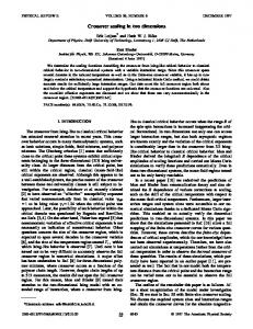
Also interesting is the distribution of domain areas, nd (A, t), which are the areas of regions of aligned spins [16]. Domains are obtained from hulls by removing any interior hulls. The domain area distribution nd (A, t) (number density of domains with area A, per unit area) of the 2dIM evolving at zero temperature after a quench from infinite temperature is shown in Fig. 3. The down-
FIG. 3: (Colour online) Number density of domains per unit area for the zero-temperature 2dIM evolving from T0 → ∞ (upper panel) and T0 = Tc (lower panel) initial conditions. In the main panels the percolating domains have been extracted from the analysis while in the insets we show the same data including the percolating clusters. We obtained the initial states after running 103 Swendsen-Wang algorithm steps. The √ full (red) line represents (5) with c = 1/8π 3 (upper) and c → c/2 (lower), and λ = 2.1 in both cases. The dotted (blue) lines have slopes -2.03 (a) and -2.05 (b).
Remarkably, the domain area distribution, nd , seems to be almost identical to the hull-enclosed area distribution nh , i.e. nd ∼ 2cd /(A + λd t)τ with a prefactor 2cd , a parameter λd and an exponent τ taking approximately the same values as for the hull-enclosed areas. An argument that treats interior domain walls in a mean-field approximation and uses the exact result for nh derived above, allows one to derive [17] nd (A, t) ∼ 2cd [λd (t + t0 )]τ −2 /[A + λd (t + t0 )]τ ,
(6)
with λd = λ + O(c), cd = c + O(c2 ) and τ ∼ 2 + O(c) for
4 infinite temperature initial conditions and, cd → cd /2 for initial conditions equilibrated at T0 = Tc . t0 is such that λd t0 = a2 , with a a microscopic length-scale, and sets the time scale. The constant cd and τ characterize the initial distribution of domain areas, nd (A, 0) ∼ 2cd aτ −2 A−τ . The exponent τ is known for the 2dIM critical geometrical clusters, τ = 379/187 ≈ 2.03 [18], and for cluster masses in 2d percolation, τ = 187/91 ≈ 2.05 [19]; the constant cd has not been computed analytically. τ > 2 allows one to satisfy the sum rule establishing that the total domain area, per unit area of the system, must be equal to unity since every spin belongs to one, and only one, domain. Unfortunately, it is hard to distinguish a power law with τ = 2 or 2.03-2.05 from our numerical data: both exponents describe the power-law tail equally well, as shown in Fig. 3, with a (blue) dotted line. It is, however, possible to put to the numerical test the value of the prefactor cd (or 2cd ) and λd . We shall present this analysis elsewhere [17]. Interestingly, similar results are obtained for the 2d random ferromagnet, at least when activation is not too important. In Fig. 4 we display data obtained at T = 0.4 after a quench from T0 → ∞. This low but finite working temperature is enough to avoid the complete pinning of domain walls by quenched disorder. Good scaling with the typical domain area R2 (t) is obtained for A/R2 (t) ≥ 10−1 and the master curve resembles strongly the one found in the pure Ising case also included in Fig. 4. 10
2
10
0
10
R(ε,t)
t1/2
-2
10
-4
10
-6
10
-8
10
1
10 10
R4(t) nd(A,t)
4
R (t) nh(A,t)
10
10
2
10
-3
10
-6
10
-9
-10
-2
-1
0
1
2
3
10 10 10 10 10 10 10
10
1
10
2
t
0
-2
10
-1
10
0
4
10
1
10
2
10
3
10
4
2
A/R (t)
FIG. 4: (Colour online) Number density of hull-enclosed and domain (lower inset) areas per unit area for the 2d random ferromagnetic Ising model with a uniform distribution of exchanges in the interval [2 − ǫ, 2 + ǫ] with ǫ = 0, 0.5, 1, 1.5, 2. The system evolves at T = 0.4 after a quench from T0 → ∞. Upper inset: the evolution of R(ǫ, t) used to scale the pdfs and its comparison to the pure R(0, t) ∝ t1/2 law.
In summary, we have obtained exact results for the statistics of hull-enclosed areas during the phase-ordering dynamics of 2d systems coarsening under curvature driven growth. Notably, these results include a proof
of the scaling hypothesis for these systems. The results are strongly supported by simulations of Ising systems, suggesting a strong degree of universality. The domain area distribution satifies a very similar law. AJB and LFC thank R. Blumenfeld, J. Cardy, D. Dhar, C. Godr`eche, S. Majumdar, P. Sollich, and R. Stinchcombe for very useful discussions. AJB and LFC thank the Isaac Newton Institute, Cambridge, and JJA the LPTHE Jussieu, Paris, for their hospitality during the period when this work was being carried out. JJA, LFC and AS acknowledge financial support from CapesCofecub research grant 448/04. JJA is partially supported by CNPq and FAPERGS and LFC by IUF.
[1] I. M. Lifshitz, Zh. Eksp. Teor. Fiz. 42, 1354 (1962) [Sov. Phys. JETP 15, 939 (1962)]. [2] S. M. Allen and J. W. Cahn, Acta Metall. 27, 1085 (1979). [3] A. J. Bray, Adv. Phys. 43, 357 (1994), and references therein. [4] W. Y. Tam, A. D. Rutenberg, B. P. Vollmayr-Lee, and K. Y. Szeto, Europhys. Lett. 51, 223 (2000), and references therein. G. L. Thomas, R. M. C. de Almeida, and F. Graner, Phys. Rev. E 74, 021407 (2006). [5] M. Marcos-Martin, D. Beysens, J. P. Bouchaud, C. Godr`eche, and I. Yekutieli, Physics A 214, 396 (1995). [6] I. Aranson and L. S. Tsimring, Rev. Mod. Phys. 78, 641 (2006). [7] M. Siegert, Phys. Rev. Lett. 73, 1517 (1994); L. Golubovic, Phys. Rev. Lett. 78, 90 (1997); D. Moldovan and L. Golubovic, Phys. Rev. E 61, 6190 (2000). [8] A. J. Bray and A. D. Rutenberg, Phys. Rev. E 49, R27 (1994); Phys. Rev. E 51, 5499 (1995). [9] J. G. Amar and F. Family, Phys. Rev. A 41, 3258 (1990); A. J. Bray, J. Phys. A 23, L67 (1990). [10] A. Coniglio and M. Zannetti, Europhys. Lett. 10, 575 (1989). [11] I. M. Lifshitz and V. V. Slyozov, J. Phys. Chem. Solids 19, 35 (1961). [12] B. Derrida and R. Zeitak, Phys. Rev. E 54, 2513 (1996). [13] A. J. Bray, B. Derrida, and C. Godr`eche, Europhys. Lett. 27, 175 (1994). [14] J. Cardy and R. M. Ziff, J. Stat. Phys. 110, 1 (2003). [15] A. D. Rutenberg, Phys. Rev. E 54, R2181 (1996) has shown that lattice anisotropy also induces a very small anisotropy in the coarsening structure. [16] See T. B. Liverpool, Physica A 224, 589 (1996) and M. Fialkowski and R. Holyst, Phys. Rev. E 66, 046121 (2002) for earlier studies of this problem. [17] J. J. Arenzon, A. J. Bray, L. F. Cugliandolo, and A. Sicilia, in preparation. [18] A. L. Stella and C. Vanderzande, Phys. Rev. Lett. 62, 1067 (1989). W. Janke and A. M. J. Schakel, Phys. Rev. E 71, 036703 (2005). [19] D. Stauffer and A. Aharony, Introduction to percolation theory, 2nd ed. (Taylor & Francis, London, 1994). [20] A. J. Bray, K. Humayun, and T. J. Newman, Phys. Rev. B 43, 3699 (1991).