arXiv:cond-mat/0205404v2 [cond-mat.dis-nn] 6 Aug 2002
Exact results for the universal area distribution of clusters in percolation, Ising and Potts models John Cardy Department of Physics Theoretical Physics, 1 Keble Road, Oxford OX1 3NP, UK & All Souls College, Oxford
[email protected] and
Robert M. Ziff Michigan Center for Theoretical Physics & Department of Chemical Engineering University of Michigan, Ann Arbor, MI 48109–2136, USA
[email protected], 734-764-5498
Abstract At the critical point in two dimensions, the number of percolation clusters of enclosed area greater than A is proportional to A−1 , with a proportionality constant C that is universal. We show theoretically (based upon Coulomb gas √ methods), and verify numerically to high precision, that C = 1/8 3π = 0.022972037 . . .. We also derive, and verify to varying precision, the corresponding constant for Ising spin clusters, and for Fortuin-Kasteleyn clusters of the Q = 2, 3 and 4-state Potts models. Key words: Percolation, Ising model, Potts model, universality, conformal field theory, Coulomb gas methods. Running title: Cluster-area distribution in percolation, Ising and Potts models.
1
1
Introduction.
It is often useful to characterize critical systems by their geometric properties, for example the distribution of cluster sizes which appears to follow a power law ns ∼ Bs−τ (1) asymptotically for large s, where ns gives the number of clusters of s connected sites, per lattice site. The exponent τ is a universal quantity whose value is the same for all systems of a given class — for example, 187 for 91 all critical percolation systems in two dimensions, no matter what lattice or percolation type is considered as long as the rules are sufficiently local. The coefficient or amplitude B however is non-universal, varying from lattice to lattice. Indeed, ns cannot have a completely universal form because it is written in terms of a lattice-level measure, the mass s. Different lattice structures have different typical site densities at the lattice level and correspondingly different values of B. In order to characterize the size distribution of clusters in a way that circumvents the site-level description, the authors of Ref. [1] considered ˜ (ℓ) (for the case of two-dimensional percolation) the quantity Nr(ℓm > ℓ) = N which gives the number of clusters whose maximum x- or y- dimension ℓm is greater or equal to a given value ℓ, divided by the total system area, A = O(L2 ). They argued that for L >> ℓ >> a (where a is the lattice spacing), this quantity should behave as C˜ ˜ N(ℓ) ∼ 2 , ℓ
(2)
with the coefficient C˜ being a universal quantity, identical for all 2d percolating system at the critical point. The universality of C˜ follows heuristically ˜ represents a macroscopic measure of the large clusters of from the idea that N the system, and remains well defined in the limit a → 0, in which the lattice disappears. The proportionality to 1/ℓ2 is a consequence of the self-similarity of the fractal percolating system, and can also be derived by the following argument (in d dimensions): from (1) it follows that the number of clusters whose mass is greater than s scales as s1−τ , and because s ∼ ℓD , where D is the fractal dimension of the clusters, the number of clusters whose length scale is greater than ℓ scales as ℓD(1−τ ) , or ℓ−d by virtue of the hyperscaling 2
relation d/D = τ −1. This result is valid for any critical system where the hyperscaling relation is valid. Later we shall give other, presumably equivalent, theoretical arguments. Besides the maximum dimension ℓm , one can consider any other macroscopic measure of the length scale of the cluster, such as the radius of gyration or the diameter of the covering disk. For each measure, there is a ˜ corresponding value of C. An equivalent way to write (2) is N(A) ∼
C A
(a2 ≪ A ≪ L2 )
(3)
where N(A) is the number of clusters (per unit area) whose area (by some measure) is greater or equal to A, and C depends upon the choice of that measure. This could be the area of the smallest disk covering the cluster, the area enclosed by the cluster, and so on. Eq. (3) is the form of the size distribution that will be considered in this paper. We note that (3) can also be written as [2] An ∼
C n
(4)
for 1 0, and similarly the contribution from a2 ∼ A ≪ L2 will violate this bound if ω < 0. Therefore ω = 0, and N(A) ∼ 2C/A for a2 ≪ A ≪ L2 . Admittedly, this argument assumes the ansatz (35), and the reader may be more comfortable with the hyperscaling argument put forward in the Introduction. However, independently of the validity of (35), our argument shows that if N(A) ∼ C/A, then the coefficient C is related to k(n). For then the leading contribution from the region a2 ≪ A ≪ L2 is 2C ln(A/a2 ) ∼ 4C ln(L/a), so that comparing once again with (28), C = k(n)/8 , (37) with k(n) given by (27). For percolation cluster hulls and FK clusters in the Q-state Potts model, √ we take n = Q = −2 cos πg in the dense phase 0 ≤ g ≤ 1, which yields g = 23 , 43 , 56 , 1 for Q = 1, 2, 3, and 4, respectively. For critical Ising spin clusters, we take n = 1 in the dilute phase where 1 ≤ g ≤ 2, so that g = 34 . Then by (27) we find the values of C given in Sec. 1 and also listed in Table 1 (taking the limit in the case Q = 4). The logarithmic corrections that appear for the case Q = 4 are derived in the Appendix.
3
Numerical results.
To test these predictions, we carried out numerical studies of percolation on square and triangular lattices with both site and bond percolation, and the Ising/Potts models on the square lattice. For percolation we considered two 13
cluster type C(measured) √ C(theoretical) Percolation 1/8 √3π = 0.022972037 . . . 0.0229721(1) Ising spin 1/16 3π = 0.011486019 . . . 0.01149(5) Ising FK 0.0265 √1/12π = 0.026525824 . . . Q = 3 Potts FK 3/20π = 0.027566445 . . . 0.0278 2 Q = 4 Potts FK 1/4π = 0.025330296 . . . 0.0258 Table 1: Predicted and measured values of C for various systems. ways to generate the clusters: populating the entire lattice, and individual hull generation.
3.1
Bond percolation — Full-lattice population method.
In the full-lattice population method, we first assign all bonds on the lattice as occupied or vacant with probabilities p or 1 − p, respectively, and then carry out all possible hull walks around these bonds. These walks go from the center to center of each bond along the diagonals, as shown in Fig. 1, and turn by an angle +π/2 when the center of an occupied bond is encountered, and by −π/2 when the center of a vacant bond is encountered. Each walk is completed when it returns to its beginning step. For bond percolation on the square lattice, we used a square lattice of size 512 × 512 with periodic boundary conditions, with p at the threshold 1/2. We simulated 107 samples, amounting to a total of 5.2 × 10¹² bonds occupied or not. We used the R9689 random number generator of Ref. [16]. In the computer program we employed an array of size 2048 × 2048, so that we had distinct array locations to represent the bonds and each diagonal leg of the hull walks. The enclosed area of a hull walk was found “on the fly” by the following method: Initially, the area is set equal to zero. When the walk steps to the right, the area is increased by one-half the y coordinate at the center of the diagonal step (where we had an array point), and decreased by one-half the y coordinate when the walk steps left. The zero point of the y coordinate is irrelevant, because its value cancels out. The factor of 1/2 comes from the fact that each leg of the hull walk changes the x-coordinate by ±1/2; we are 14
111111111111111111111111 000000000000000000000000 111111111111111111111111 000000000000000000000000 11 00 11111 00000
111111111111111111111111 000000000000000000000000 000000000000000000000000 111111111111111111111111 111111111111111111111111 000000000000000000000000 Figure 1: Hull paths for bond percolation, with enclosed shaded areas of 12 (top left), 1 (top right), 2 (bottom left) and 2 12 (bottom right). These are all external hulls – the last case also has an internal hull of area 12 (not shown).
15
taking the spacing of the bond lattice to be unity. When the walk closes, this algorithm gives the area of the enclosed space, with a sign attached: positive areas correspond to external hulls that surround clusters, and negative areas corresponds to internal hulls (which are of course external to the clusters on the dual lattice). The smallest area is 1/2; for positive area this corresponds to the hull around an isolated site (one with no bonds attached), and negative 1/2 corresponds to the hull inside a square of four occupied bonds, or equivalently around an isolated site on the dual lattice. The area of all the hulls are in √ units of 1/2. (Alternately, one could consider the lattice spacing to be 2; then the hulls would all have integer areas, and the system area would be 2L2 .) Because we use periodic boundary conditions, there is the possibility that some hulls could wrap around the torus once or more before closing into a loop. The areas for such loops are undefined, unless taken in pairs, but in any case we discarded them because we are interested in clusters whose size is much smaller than the size of the system. We found the statistics for internal and external hulls were identical (within numerical error), as one would expect for this self-dual system, and took the average of the two. For small A we kept track of the quantity NA = the number of loops (per unit area) whose enclosed area is exactly A, where A = 12 , 1, 32 , 2, .... According to (3), this quantity should behave as NA = N(A) − N(A + 1/2) ∼
C 2A2
(38)
so that 2A2 NA ∼ C for large A. The results are given in Table 3 for A ≤ 5. To check these results, we derived the exact expressions for NA for 21 ≤ A ≤ 92 given in Table 2. These are for an arbitrary bond occupancy of p, with q = 1 − p. For A = 12 . . . 3 these expressions are identical to the expressions for the number of clusters (per site) containing b = 2A − 1 bonds, which are well known [17, 18]. For larger A we had to make modifications to the bond cluster expressions to take into account graphs that contain internal open spaces with vacant bonds, which result in areas larger than (b + 1)/2. We subtracted the term 2p6 q 11 from N 7 and added it to N4 to account for the area 2 of an open 1 × 2 rectangle, whose external hull area is 4, not 7/2. Likewise, the term 20p7 q 13 (the 1 × 2 rectangle with an extra bond attached) was 16
A 1 2
1 3 2
2 5 2
3 7 2
4 9 2
NA (p) q4 2pq 6 6p2 q 8 p3 (4q 9 + 18q 10 ) p4 (q 8 + 32q 9 + 55q 10 ) p5 (8q 10 + 30q 12 + 160q 13 + 174q 14) p6 (12q 11 + 40q 12 + 332q 14 + 672q 15 + 570q 16 ) 2p6 q 11 + p7 (2q 10 + 136q 13 + 168q 14 + 336q 15 + 2030q 16 + 2712q 17 +1908q 18) 20p7q 13 + p8 (22q 12 + 186q 14 + 844q 15 + 868q 16 + 4064q 17 + 9972q 18 +10880q 19 + 6473q 20 )
Table 2: Exact results for NA (p) for bond percolation on the square lattice at occupancy p = 1 − q, for A = 12 . . . 92 . subtracted from N4 and added to N9/2 . Finally, the terms 42p8 q 14 , 114p8 q 15 , and p8 q 16 , which correspond to various graphs with area greater than 9/2, were subtracted from N9/2 . These various diagrams are shown in Fig. 2. This shifting of terms has the effect of making NA follow asymptotically the exponent −2 of (38) rather than the exponent −τ = −2.055 . . . followed by ns . Taking p = 1/2 and multiplying by 2A2 , we arrive at the estimates for C listed in Table 3. The agreement with our numerical results is excellent — within the small statistical error. Interestingly, the convergence of these estimates is rather quick — already, at A = 5, the result is within 6% of the (presumably) exact value. To analyze the data for larger A, we considered the quantity N(A, 2A) ≡ the number of clusters whose enclosed area is greater or equal to A and less than 2A. According to (3), this quantity should behave as N(A, 2A) = N(A) − N(2A) ∼
C 2A
(39)
so that 2AN(A, 2A) ∼ C for large A. The measured values of 2AN(A, 2A) are given in Table 4. They monotonically decrease to a value 0.0229860(45) for A = 2048, but then slightly increase at A = 4096; for larger A, the increase continues, as seen in Fig. 17
2p6q11 A=4 20p7q13 A = 9/2
42p8q14 A=5
114p8q15 A=5
p8q16 A = 13/2 Figure 2: Clusters contributing higher-area terms to polynomials in Table 2. Solid lines represent occupied bonds, dashed lines are vacant bonds, and the dotted lines trace out the external hull. These are the graphs that have to be “moved” in the usual cluster polynomials from A = (b + 1)/2 (where b is the number of bonds) to higher A due to the existence of enclosed open spaces.
18
0.02315
2 A N(A,2A)
0.0231
0.02305
0.023
0.02295
0.0229
0
0.01
0.005 A
0.015
-0.875
Figure 3: Plot of 2AN(A, 2A) vs. A−0.875 for bond percolation on a square lattice. Upper data points: lattice population method. Lower points (shifted down by 0.00005): single hull generation method.
19
A 1/2 1 3/2 2 5/2 3 7/2 4 9/2 5
Full lattice 0.0312500(1) 0.0312500(1) 0.0263674(1) 0.0253907(2) 0.0257491(2) 0.0254749(3) 0.0249188(3) 0.0249898(4) 0.0247714(4) 0.0245659(5)
Single Exact hull results 0.031247(3) 1/32 = 0.03125 0.031252(4) 1/32 = 0.03125 0.026363(4) 27/1024 = 0.026367188 0.025398(5) 13/512 = 0.025390625 0.025744(6) 3375/217 = 0.025749207 0.025477(6) 3339/217 = 0.025474548 0.024917(7) 104517/222 = 0.024918795 0.025004(7) 6551/218 = 0.024990082 0.024778(8) 13298985/229 = 0.02477129 0.024557(8)
Table 3: Values of 2A2 NA for small A for bond percolation on the square lattice: two algorithms and exact results. Errors in last digit are given in parentheses. 3, (upper curve) where the data from A = 128 to 16384 are shown. We attribute this increase to interference of clusters with themselves around the periodic boundary conditions, and thus ignore these data. Fitting the the 5 data points from A = 128 to 2048 as a function of A−θ to a straight line, we find a good linear fit with θ = 0.875 as shown in that figure, with the equation of the line given by 2AN(A, 2A) = 0.0229712 + 0.01148A−0.875
(40)
implying C = 0.0229712. We estimate the error in the above value of C to be ≈ 10−6 from the statistical error of the data and the uncertainty in the extrapolation to infinity. The predicted value (5) falls within these error bars. 1 In terms of the length scale ℓ ∼ A 2 , this exponent corresponds to a correction of the order ℓ−1.75 , which is the scaling of the hull of the cluster. Indeed, this finite-size correction can be interpreted as a surface effect [19], reflecting the arbitrariness in locating where precisely the hull of the cluster should be placed. 20
As a test of our procedure, we also compared our measurement of the total number of loops (hulls of both type) per unit area (≈ twice the number of clusters) with the theoretical result, which for bond percolation on the square lattice is given by the Temperley-Lieb result [20, 21] X √ NA ∼ 3 3 − 5 = 0.196152422 . . . (41) A
Our measured value was 0.1961572(14), larger than the above prediction by only 0.0000048(28). This difference corresponds to an excess number of 1.2 loops per lattice (found by multiplying the latter number by 5122 ), which is barely discernible above the statistical error of ±0.7. In fact, this correction can also be predicted theoretically. For a system with a rectangular boundary of aspect ratio r, the excess number of clusters is a known function b(r) [21, 22]. To find the excess number of loops, note that the quantity nc + nc′ − nl (the number of clusters, plus the number of dual lattice clusters, minus the number of loops) equals 1 if there is a cross-configuration on the lattice or the dual lattice, and zero otherwise. Thus it follows that the excess number of loops is just 2b(r) − 2π+ (r), where π+ (r) is the cross-configuration probability, which has been calculated by Pinson [23]. For a square system, the excess number of loops is predicted to be 2[b(1) − π+ (1)] = 2(0.883576 − 0.309526) = 1.14810
(42)
using b(1) from [22] and π+ (1) from [1]. This prediction happens to coincide almost exactly with the measured value (even though the error bars of the latter are quite large). This predicted value can be tested to higher precision most easily by going to smaller lattices. Besides the problem of clusters interfering with themselves, there is also the problem in the population method that the statistics for larger hulls are rather poor because of the relatively small number of such hulls that are generated. In the next section we consider a method that addresses both of these problems.
3.2
Bond percolation — Single hull generation method.
It is well known that percolation clusters can be grown individually through a process where bonds are made occupied or not only when they are encountered (the “Leath” method). In the same way, percolation hulls can be 21
A
Full lattice 1/2 0.0625001(1) 1 0.0429689(1) 2 0.0306645(2) 4 0.0270220(2) 8 0.0250527(3) 16 0.0240647(4) 32 0.0235504(6) 64 0.0232785(8) 128 0.0231360(11) 256 0.0230598(16) 512 0.0230218(22) 1024 0.0229968(32) 2048 0.0229860(45) 4096 0.0229882(63)
Single hull 0.0625022(42) 0.0429634(32) 0.0306677(26) 0.0270226(25) 0.0250528(25) 0.0240635(25) 0.0235463(26) 0.0232740(27) 0.0231412(28) 0.0230616(29) 0.0230212(31) 0.0229948(32) 0.0229849(33) 0.0229785(35)
Table 4: Values of 2AN(A, 2A) for bond percolation on the square lattice for the two algorithms.
22
generated individually on a blank (undetermined) lattice by a kind of growing self-avoiding walk that mimics the walk used to trace out hulls [24]. For critical bond percolation [25], the walker moves along the edges of a square lattice (the diagonals in Fig. 1), and turns by +π/2 or −π/2 randomly at each vertex, except at vertices previously visited, where it always turns to avoid retracing itself. The walk terminates when it returns to the origin and cannot proceed further. Note that pseudo-random numbers are generated only for the bonds that are visited during the walk, making this method efficient. This walk has also been studied as a kinetic Lorentz-gas model [26], and the results here apply to that model also. In order for the contribution of a given hull to be the same as on the fully populated lattice, it is necessary to weight each walk by 1/t, where t is the number of hull steps. This compensates for the fact that a hull of t steps is generated with t times the probability in the single cluster method compared to the population method, because there are t places a given walk can start from. This weighting can also be checked as follows: The probability of generating a closed hull of at least t steps is generated with a probability [27] P (t) ∼ ct−1/7
(43)
where c is a constant. Defining a Euclidean length scale ℓ ∼ t1/DH , it follows that the area enclosed by the walk scales as A ∼ ℓ2 ∼ t2/DH = t8/7 . Thus, the probability of growing a walk enclosing at least area A scales as A−1/8 , so that the probability of growing a walk of exactly area A scales as A−9/8 . When we weight a hull by the factor 1/t ∼ A−7/8 , we thus get the proper probability A−9/8−7/8 = A−2 as given in (38). In our simulations, we considered square lattices of size L × L with periodic b.c. This is the lattice of the hull walks, which √ is rotated by π/4 from the square bond lattice, and has a spacing that is 2/2 of the bond lattice spacing. Note that the square system boundary here corresponds to a diamond on the bond lattice. We stopped all walks that did not close by 65536 steps, and kept track of the areas of all the walks that closed before this cutoff, without wrapping around the periodic b.c. With this cutoff, we could be assured that all walks that were stopped at the cutoff would ultimately enclose an area of at least 65536/8 = 8192, taking into account that there are at most 4 hull steps around each wetted site, and each square on the hull-walk (rotated) lattice corresponds to an area of 1/2. 23
While the statistics of walks of areas smaller than A = 8192 should thus be unbiased by having this cutoff, they can still be biased by the finite-size of the lattice. For runs on lattices of size 1024 × 1024 and smaller, we found both wraparound clusters and large deviations in the hull statistics for larger A. Even for lattices of size 2048 × 2048, where no wraparound occurred with this cutoff, we still found significant, obviously finite-size deviations even for N(A, 2A) for A below A = 8192. We attribute these deviations to hulls making contact with themselves around the periodic b.c., without actually closing to wrap around. Therefore, to be absolutely certain of no finite-size effects, we went to a lattice of size 65536 × 65536 using the virtual lattice method of [24]. We checked that with the cutoff of 65536 steps, indeed no walk got anywhere near the boundary of the system. We carried out 1.8 × 10⁹ walks on this lattice, which, like the simulations for the 107 fully populated lattices, took several weeks of workstation computer time. A total of 3.2 × 10¹³ hull steps simulated here, compared with 1.0 × 10¹³ in the simulations of the populated lattices. The algorithm for the single-hull method is somewhat simpler and more efficient than that for the lattice population method. In the single-hull method, larger hulls are generated with a higher probability than in the lattice-population method: the number generated in the interval (A, 2A) (before reweighting) is proportional to A−1/8 here, compared with A−1 . This is advantageous because the large hulls with their small finitesize effects are essential for finding C accurately. On the other hand, in the single-hull method a large fraction of time is spent on the walks that reach the cutoff before they close (and are discarded): Eq. (43) implies that the total number of steps for all the hulls that reach the cutoff tmax grows as ∼ c t6/7 max , while the total number of steps for all the hulls that close before tmax is given by ! Z tmax dP c t − dt ∼ t6/7 . (44) dt 6 max Thus, no matter what the value of the cutoff is, a fraction 6/7 = 85.7 % of the work (ignoring finite-size effects) is spent generating walks that reach the cutoff without closing and are thus discarded. Still, for very large cutoffs this overhead is compensated by the increase in useful statistics for large A, making this method advantageous. Note that, in our simulations of 3.2 × 10¹³ hull-walk steps, the fraction 24
of those steps belonging to clusters that reached the cutoff tmax = 65536 was 6.000124/7, with the deviation from 6 in the numerator being about equal to the apparent statistical error, ≈ 0.0001. This result seems to provide a very precise confirmation that the exponent in P (t) is indeed −1/7 (i.e., the hull fractal dimension is DH = 7/4), although to quantify the precision of this result one would have to investigate different values of the cutoff tmax to determine the finite-size corrections. For small A, results for 2A2 NA are given in Table 3 agree with the exact values, confirming that the 1/t weighting is correct. Because the single hull method gives fewer of these small hulls than the lattice population method, these results have larger error bars. Here use used (NA (total))−1/2 , where NA (total) is the total number of clusters of size A, to estimate the error bars. Likewise, the results for N(A, 2A) for all A, given in Table 4, are seen to agree with the lattice population results. For the largest size ranges, the single-hull method is seen to give better error bars (and are not biased by finite-size boundary effects). A plot of the 2AN(A, 2A) vs. A−0.875 for 128 ≤ A ≤ 4096 is also given in Fig. 1 (shifted down by 0.00005), and the data are fit by the linear function given y 2AN(A, 2A) = 0.0229692 + 0.01197A−0.875 (45) which is consistent with the results of the lattice population method (40). The error bars on the intercept is about the same, 10−6 . Thus, although the single-hull method is in principle advantageous, for the system size we considered we obtained C with about the same precision as the lattice population method, with about the same amount of work. However, the single-hull method allowed us to show that the curvature in the behavior of 2AN(A, 2A) for large A as seen in Fig. 1 was indeed due to cluster interference around the periodic boundaries. Assuming the predicted value of C given by (5), we can also make a plot of log(2AN(A, 2A) − C) vs. log(A) (not shown); with single-hull data we find good linear behavior with a slope −θ = −0.88±0.01, which is consistent with the value 0.875 that we have been using.
25
(a)
0000000000000000000 1111111111111111111 0000 1111 0000 1111 1111111111111111111 0000000000000000000 00000000 11111111 000000000 111111111 00000000 11111111 000000000 111111111 0000 1111 0000 1111 00000000 000000000 111111111 00000000 11111111 000000000 111111111 (b) 11111111 0000 1111 0000 1111 00000000 11111111 000000000 111111111 00000000 11111111 000000000 111111111 0000 1111 0000 1111 00000000 11111111 000000000 111111111 00000000 11111111 000000000 111111111 0000 1111 00000000 11111111 000000000 111111111 00000000 11111111 000000000 111111111 0000 1111 1111111111111111111 0000000000000000000 0000 1111 0000 1111 00000000 11111111 000000000 111111111 00000000 11111111 000000000 111111111 0000 1111 0000 1111 00000000 11111111 000000000 111111111 00000000 11111111 000000000 111111111 0000 1111 00000000 11111111 000000000 111111111 00000000 11111111 000000000 111111111 0000 1111 1111111111111111111 0000000000000000000 0000 1111 0000 1111 00000000 11111111 000000000 111111111 00000000 11111111 000000000 111111111 0000 1111 0000 1111 00000000 11111111 000000000 111111111 00000000 11111111 000000000 111111111 0000 1111 0000 1111 00000000 11111111 000000000 111111111 00000000 11111111 000000000 111111111 0000 1111 0000 1111 1111111111111111111 0000000000000000000 00000000 11111111 000000000 111111111 00000000 11111111 000000000 111111111 0000 1111 0000 1111 00000000 11111111 000000000 111111111 00000000 11111111 000000000 111111111 0000 1111 0000 1111 00000000 11111111 000000000 111111111 00000000 11111111 000000000 111111111 0000 1111 0000 1111 00000000 11111111 000000000 111111111 00000000 11111111 000000000 111111111 1111111111111111111 0000000000000000000
(c)
Figure 4: Medial lattices used for hulls in site percolation: (a) square lattice, (b) triangular lattice, and (c) brick-lattice form of triangular lattice.
26
3.3
Site percolation on the square and triangular lattices.
We also carried out simulations of site percolation on two different lattices to demonstrate the universality of the result (5) for C. For site percolation, the logical choice for the hull walk around a cluster is to follow a path on the medial lattice whose vertices are at the center of the faces of the lattice, as shown in Fig. 4 for the square and triangular lattice. This choice allows the single isolated site to have a non-zero area, and is symmetric for internal and external hulls for the triangular lattice. For the square lattice, we carried out 4 × 10⁸ samples on a lattice of size 256 × 256, using the weighted single-hull method. (In our program we employed a computer array of size 512×512 to include the sites of the medial lattice.) With such a small lattice, finite-size effects appeared for hulls with A larger than ≈ 1024. We used occupancy probability p = 0.592746, which is close to the critical threshold for this system [28]. Here we generated the hulls starting from a segment between a single occupied and vacant site, which occurs in a populated system with a probability of p(1 − p). The latter factor was therefore included in the total weight of each hull, along with the 1/t weight, where here t is the number of steps along the medial lattice. We found that the statistics for internal and external hulls are quite different, as one would expect by the asymmetry of this system. For example, for A = 1, N1 = p(1 − p)4 ≈ 0.0163053 for an external hull, and N1 = (1 − p)p8 ≈ 0.00620604 for an internal hull. This large difference persists as A increases, and suggests that some other definition of the hull which gives more symmetric results between external and internal hulls might be advantageous. In Fig. 5 we show 2AN(A, 2A) for the two kinds of hulls, along with their average. Taking the average is the same as including both types of hulls in the area calculation (and dividing by two). Indeed, in the theoretical development in Section 2, both internal and external hulls were included in the calculation, so it is appropriate to take this average. The finite-size corrections to the average measure again followed a behavior with exponent close to −0.875, which was used in the plot in Fig. 5. The line in that figure is fit by the equation 2AN(A, 2A) = 0.022976 − 0.0114A−0.875 27
(46)
0.028
0.026
2 A N(A,2A)
0.024
0.022
0.02
0.018
0.016
0
0.02
0.04
0.06 A
0.08
0.1
-0.875
Figure 5: Plot of 2AN(A, 2A) vs. A−0.875 for site percolation clusters on a square lattice: external hulls (triangles), average (circles) and internal hulls (squares). The equation of the line fit through the average points is given in Eq. (46). where the unit of area is one square lattice spacing on the square lattice. The average measure extrapolates (for large A) to a value ≈ 0.022976, in obvious agreement with the theoretical prediction, and making a more precise determination rather superfluous. Note that, the coefficient to the correction term is similar in value to the coefficient for bond percolation, even though a different kind of path was used to define the hulls in the two cases. The similarity might be a coincidence, or it might reflect a fundamental equivalence of perimeter corrections for site and bond percolation on this lattice. For site percolation on the triangular lattice the medial lattice is a honeycomb lattice with a hexagon around each vertex of the triangular lattice as shown in Fig. 4. To implement this in the computer, we used the squarelattice form of the honeycomb lattice, also shown in that figure, where the hexagons become rectangular bricks and a single site on the triangular lattice 28
now becomes a pair of sites on the square lattice. Thus, we could use the same basic algorithm as we used for site percolation on the square lattice, with the only modification being that sites are occupied or made vacant in pairs, with a probability 1/2. For this case (the triangular lattice) we used the lattice-population method on an underlying square lattice of size 1024 × 1024 with periodic b.c. We generated 2.4 × 10⁶ independent samples. As expected, the internal and external hulls had equal statistics, within error, reflecting the symmetry of this system. Again, the data closely followed the A−0.875 behavior, and we do not plot it. Fitting the data in the range 26 < A < 212 (where A is measured in square-lattice units, so that the smallest hexagon corresponds to A = 2) we found the following behavior: 2AN(A, 2A) = 0.022977 − 0.0146A−0.875
(47)
again agreeing with the predicted value of C. In this case, that value is approached from below for finite systems, with the definition of cluster-hull area used here.
3.4
Ising clusters.
To study the clusters of the Ising model, we considered a square lattice of size 1024 × 1024 with periodic b.c., and simulated the system at the critical √ temperature of exp(−J/kT ) = 1 + 2 (where J is the coupling constant in P the Potts model formulation, H = −J δσi δσj ) using the Wolff variation [29] of the Swendsen-Wang method [30]. We initialized the lattice with 1000 updates, and then measured the hull area distribution treating the system exactly as if it were one of site percolation, using the same definition of hull areas as shown in Fig. 2 and indeed the same algorithm. This was followed by 10–100 Wolff updates, and the procedure was repeated. 140,000 realizations were generated. As in the site percolation case, we found rather large differences between internal and external hulls, as seen in Fig. 6. Here we also found very large deviations for large A, presumably reflecting stronger correlations due to the interaction. (Indeed, runs on a smaller 256×256 lattice showed even stronger large-A deviations.) The average measure for the smaller hulls is consistent 29
0.014
0.0135
2 A N(A,2A)
0.013
0.0125
0.012
0.0115
0.011
0
0.05
0.1
0.15
0.2
0.25
−0.875
A
Figure 6: Plot of 2AN(A, 2A) vs. A−0.875 for Ising clusters: external hulls (triangles), average (circles) and internal hulls (squares). The line is fit through the four rightmost points of the average values.
30
with the A−0.875 finite-size scaling used in that figure, and a fit of the points for A = 2 through 16 yields the straight line as shown in that figure, with a fit of 2AN(A, 2A) = 0.011487 + 0.004458A−0.875 (48) The intercept is nearly identical with the predicted value of C (6), in spite of the rather small size of clusters that were used. We estimate the error to be ±0.00005.
3.5
FK Clusters on the Potts model for Q = 2, 3 and 4.
We also studied the FK clusters on the Potts model at the critical temper√ ature eJ/kT = 1 + Q. These clusters are the bond percolation clusters when bonds are drawn between neighboring identical spins with a proba√ √ bility 1 − e−J/kT = Q/(1 + Q). We defined the hulls exactly as in the square-lattice bond percolation case (Fig. 1) and indeed could use the same algorithm to trace out and measure the hulls after the bonds have been specified. To thermalize the system, we used the Swendsen-Wang (SW) procedure of identifying all FK clusters on the lattice and then randomly reassigning their spins. Indeed, the FK hull measurements and the SW update method naturally go hand in had in this calculation, since the identification of the FK clusters is needed for the SW method. For Q = 2 and Q = 3 we used a lattice of size 512 × 512 and obtained the results shown in Figs. 7 and 8, where once again we find large discrepancies between internal and external clusters, and take the average of the two. That average is found to fall on a nearly straight line when plotted as a function of A−θ taking θ = 0.875 for Q = 2 and θ = 0.7 for Q = 3. The extrapolated exponents are seen to approach the expected theoretical values, as shown in Table 1. We simulated 82, 000 samples (Q = 2) and 1,000,000 samples (Q = 3). Note that the discrepancy between internal and external hulls reflects an inherent asymmetry for FK clusters of the Potts model in finite periodic systems for Q > 1. This asymmetry is also manifested in the behavior of the fraction of bonds that are occupied, which in finite systems has a value somewhat greater than the infinite-system value of 12 [31]. For Q = 4, very large differences between internal and external hulls 31
0.04
2 A N(A,2A)
0.035
0.03
0.025
0.02
0
0.1
0.05
A
0.15
0.2
-0.875
Figure 7: Plot of 2AN(A, 2A) vs. A−0.875 for FK clusters of the Ising model (Q=2 Potts): external hulls (triangles), average (circles) and internal hulls (squares).
32
0.04
2 A N(A,2A)
0.035
0.03
0.025
0.02
0
0.05
0.1
0.15 A
0.2
0.25
-0.7
Figure 8: Plot of 2AN(A, 2A) vs. A−0.7 for FK clusters of the Q=3 Potts model: external hulls (triangles), average (circles) and internal hulls (squares).
33
persisted even for relatively small values of A on the 512 × 512 lattice, so we went to a larger lattice of size 2048 × 2048 (20,000 realizations) which improved the behavior somewhat. Even for this lattice, however, large finitesize effects were apparent. Similar large finite-size corrections have been seen in other Potts model studies at Q = 4 (e.g., [31, 32]) and are generally expected to be logarithmic in character. In the Appendix we have calculated these corrections analytically for this case and find 2a2 C 1− + O((ln A)−3 ) N(A) ∼ 2 A (ln A)
!
(49)
where a2 is a constant. The above result implies that 2AN(A, 2A) = C + O((ln A)−2 ). In Fig. 9 we plot our results for 2AN(A, 2A) as a function of (ln A)−2 . The data fall on a straight line for large A, and the intercept yields C = 0.0258, which is comparable to our predicted value of 1/4π 2 = 0.0253 . . .. Note that if we plot the data versus 1/ ln A, we find about as good of a fit to linear behavior for large A, but then the intercept would 0.0231, quite a bit below the predicted value of C. Likewise, if we fit the data to a power-law as we did for other values of Q, we find fairly linear behavior with an abcissa of A−0.5 , but now the intercept is 0.0279. Thus, the data is consistent with our prediction for C combined with the predicted 1/(ln A)2 finite-size scaling.
4
Conclusions.
We derived and numerically confirmed predictions for the behavior of the area-size distribution of various Potts model including percolation clusters. For the latter, we also considered different lattices and percolation types (site and bond) to demonstrate universality. The theoretical ideas presented in Section 2 were well verified numerically, especially in the percolation and Ising model cases. For Q = 4, our results were consistent with the logarithmic finite-size behavior predicted here. This work confirms the idea of a universal size distribution expressed by Eq. (3). An alternate way to state that result is as follows: Consider that the unit of area is now some value A much smaller than the lattice size (which is therefore no longer of unit area). Then, (3) implies that the number of clusters whose enclosed area is greater than A, per unit area A, is a constant
34
0.04
0.035
2 A N(A,2A)
0.03
0.025
0.02
0.015
0.01
0
0.05
(ln A)
-2
0.1
0.15
Figure 9: Plot of 2AN(A, 2A) vs. (ln A)−2 for FK clusters of the Q=4 Potts model: external hulls (triangles), average (circles) and internal hulls (squares).
35
C, for all values of A. The lack of dependence on A is a direct consequence of the scale-free nature of this fractal system. The arguments put forward in Sec. 2.1.2 also imply that the number of cluster hulls which must be crossed to connect a typical point deep inside the system to the boundary behaves as 4C ln(L/a), where L is the system size, with same value of C for each universality class. So, for example, the fact that C for critical Ising spin clusters is half that for percolation clusters means, according to Zipf’s law, that the nth largest cluster is the Ising case has roughly half the area of the nth largest percolation cluster. This is consistent with the fact that we have to cross one half as many cluster hulls to reach the boundary in the Ising case. It might suggest that we may go from the ensemble of percolation hulls to those of Ising clusters simply by erasing every other percolation hull, e.g. by ignoring all the internal hulls! This however is not the case, as percolation hulls have a different fractal dimension from those of Ising clusters. The form of (3) is also consistent with the existence of the universal amplitude ratio, Rξ+ = [α(1 − α)(2 − α)Fc ]1/d ξ0 , where α is the free-energy critical exponent, Fc is the critical part of the free energy per unit area, and ξ0 is the amplitude for the correlation length [33]. For any value of Q in the random cluster model, ∂F /∂Q gives the mean total number of clusters P P per unit area s ns = A NA . At the critical point, NA ∼ −N ′ (A) ∼ C/A2 for A ≫ a2 , and near the critical point one expects a scaling law NA = A−2 Φ(A/ξ 2 ), where Φ(u) is some nontrivial scaling function with Φ(0) = C, which decays exponentially fast as u → ∞. This gives, on substitution into R∞ P A NA ∼ a2 NA dA, X ns ∼ const. + Bξ −2 (50) s
where the constant is nonuniversal, as it depends on the details of the cutoff, and Z ∞ Φ(u) − C B= du . (51) u2 0 Eq. (50) is of the form expected from hyperscaling [33], with B = (Rξ+ )2 /]α(1− α)(2 − α)] directly related to the universal combination Rξ+ (recently given exactly for percolation by Seaton [34]). However, we see that it is given by a certain integral over a nontrivial scaling function, while C is just one limiting value of this function.
36
The results presented here represent the first examples where a measure of the cluster size distribution is given exactly (in the asymptotic limit), both in exponent (here, simply −1) and amplitude (the value C). The agreement between the theoretical prediction and the numerical results for percolation (to a relative accuracy of better than 10−4 ) compares well with other precision tests of conformal field theory predictions for percolation amplitudes, for example the crossing formula [37] (where the results have been confirmed within a relative error of about 10−3 [35, 36]). Knowing the exact result for C at the critical point allows finite-size effects and behavior away from the critical point to be studied, without at the same time having to determine these critical parameters. In percolation especially there has been great interest in size distributions and their finite size corrections, so this result should be useful in that field.
5
Acknowledgements
J. C. thanks H. Kesten for useful comments and for drawing attention to Refs. [14, 15]. He was supported in part by EPSRC Grant GR/J78327. R. Z. acknowledges a discussion with Greg Huber concerning the origin of the finite-size corrections.
Appendix. Logarithmic corrections for Q = 4. We summarize the arguments leading to Eq. (49). It has long been known that many critical quantities in the 4-state Potts model exhibit confluent logarithmic corrections. In the RG framework, this is explained by the existence of a marginally irrelevant scaling variable [38]. A general formalism for computing the form of these corrections was developed in Ref. [39], was taken further in Ref. [40], and recently has been applied to the fractal properties of Q = 4 FK clusters by Aharony and Asikainen [41]. In general [39], logarithmic corrections to susceptibilities take the form of multiplicative powers of logarithms, and are therefore numerically very significant, but in some quantities, for example the finite-size scaling of the free energy at the critical point [42], they give only additive corrections. We shall argue that this is the case here.
37
Following [42], suppose that the fixed-point hamiltonian is deformed by a P marginal perturbation H∗ → H∗ + g R Φ(R), where Φ is a scaling operator with scaling dimension xΦ = 2. We may develop the current-current correlation function (18 in a power series in g, the coefficient of each term being a sum over the Rj of correlation functions hJµ (r1 )Jν (r2 )Φ(R1 )i, hJµ (r1 )Jν (r2 )Φ(R1 )Φ(R2 )i, and so on, each evaluated with respect to the fixed point hamiltonian. The form of the r1 and r2 -dependence of each of these correlation functions is completely fixed by conformal invariance in two dimensions, so that they may be computed in a simple model. Choosing a gaussian theory with hamiltonian 1 R ∗ H = 2 (∂φ)2 d2r, a conserved current Jµ ∼ ∂µ φ, and the marginal operator Φ ∼ (∂φ)2 , all the correlators may be evaluated using Wick’s theorem. For the O(g) correction, it turns out that the only non-zero components (in complex coordinates) have µ = z, ν = z¯, and vice versa. The form of the correlation function is hJz (z1 )Jz¯(¯ z2 )Φ(0)i ∝ 1/(z12 z¯22 )
(52)
where we have set R1 = 0 for convenience. Now the O(g) correction to the total area within all loops (15) is g
Z
hJy (z1 )Jy (¯ z2 )Φ(R1 )i|x1 − x2 |δ(y1 − y2 )dx1 dx2 dy1dy2 d2R1
(53)
where Jy ∝ Jz − Jz¯. This is to be evaluated in a large but finite region of linear size O(L). As before, we shall use the infinite volume continuum limit form (52) of the correlation function, justifying this a posteriori. The integral in (53) is then proportional to the area A of the system, and we remove this factor by setting R1 = 0. The remaining integral is then proportional to Z
∞
−∞
|x1 − x2 | dx1 dx2 dy1 (x1 + iy1 )2 (x2 − iy1 )2
(54)
The contour integration over y1 vanishes unless x1 and x2 have the same sign: the result is then proportional to Z
0
∞
Z
0
∞
|x1 − x2 | dx1 dx2 = (x1 − x2 )3
Z
dx1 ∼ ln(L/a) x1
(55)
with an equal contribution from x1 , x2 < 0. We have cut off the logarithmically divergent integral in the last step, arguing that because the divergence 38
is only logarithmic, it was permissible to use the infinite-volume forms for the correlation function in the integrand. The important point about this result is that it is O(g ln L), not O(g(ln L)2 ), as might have been expected (recall that the leading term is O(g 0 ln L)). A similar, but more tedious, calculation shows that the next term is O(g 2 ln L), and we conjecture that the nth order term is O(g n ln L). This is consistent with the fact that, in the gaussian model, g is exactly marginal so that k, the coefficient of the O(ln L) term, depends continuously on g. However, in the 4-state Potts model the perturbation is not exactly marginal, and instead flows logarithmically slowly to zero under the RG. This may be taken into account [42] by replacing the bare expansion parameter g by the running coupling g˜(L) =
g ∼ (b ln L)−1 + O(g −1(ln L)−2 ) 1 + bg ln L
(56)
where b is a known constant whose value is not important. Inserting this result into the formula (15) for the total area hAtot i ∼ P A A