Preprints of the 18th IFAC World Congress Milano (Italy) August 28 - September 2, 2011
Exact Tuning of PID Controllers in Control Feedback Design ★ L. Ntogramatzidis ∗ A. Ferrante ∗∗ ∗ Department
of Mathematics and Statistics, Curtin University, Perth WA 6845, Australia. (E-mail:
[email protected]). ∗∗ Dipartimento di Ingegneria dell’Informazione, Universit` a di Padova, via Gradenigo, 6/B – I-35131 Padova, Italy. (E-mail:
[email protected]) Abstract: In this paper, we introduce a range of techniques for the exact design of PID controllers for feedback control problems involving requirements on the steady-state performance and standard frequency domain specifications on the stability margins and crossover frequencies. These techniques hinge on a set of simple closed-form formulae for the explicit computation of the parameters of the controller in finite terms as functions of the specifications, and therefore they eliminate the need for graphical, heuristic or trial-and-error procedures. The relevance of this approach is i) theoretical, since a closed-form solution is provided for the design of PID-type controllers with standard frequency domain specifications; ii) computational, since the techniques presented here are readily implementable as R ; iii) educational, because the synthesis of the controller software routines, for example using MATLAB⃝ reduces to a simple exercise on complex numbers that can be solved with pen, paper and a scientific calculator. These techniques also appear to be very convenient within the context of adaptive control and self-tuning strategies, where the controller parameters have to be calculated on-line. 1. INTRODUCTION Countless tuning methods have been proposed for PID controllers over the last seventy years. Accounting for all of them goes beyond the possibilities of this paper. We limit ourselves to noticing that many surveys and textbooks have been entirely devoted to these techniques, that differ from each other in terms of the specifications, the amount of knowledge on the model of ˚ om et al. the plant and in terms of tools exploited, see e.g. Astr¨ (1995); Datta et al. (2000); Visioli (2006) and the references therein. Recently, renewed interest has been devoted to design techniques for PID controllers under frequency domain specifications, see e.g. Yeung et al. (2000); Skogestad (2003); Keel et al. (2008); Ho et al. (1995). In particular, much effort has been devoted to computation of the parameters of the PID controllers that guarantee desired values of the gain/phase margins and of the crossover frequency. Specifications on the stability margins have always been extensively utilised in feedback control system design to ensure a robust control system. It is also common to encounter specifications on phase margin and gain crossover frequency, since these two parameters together often serve as a performance measure of the control system. In the last fifteen years, three important sets of techniques have been proposed to deal with requirements on the phase/gain margins and on the gain crossover frequency, to the end of avoiding the trial-and-error nature of classical control methods based on Bode and Nichols diagrams. The first one is a graphical method hinging on design charts, and exploits an interpolation technique to determine the parameters of the PID controller. This ★ This work was partially supported by the Australian Research Council (Discovery Grant DP0986577) and by the Italian Ministry for Education and Resarch (MIUR) under PRIN grant “Identification and Robust Control of Industrial Systems”.
Copyright by the International Federation of Automatic Control (IFAC)
method can deal with specification on the stability margins, crossover frequencies and on the steady-state performance, Yeung et al. (2000). A second important set of techniques that can handle specifications on the phase and gain margins relies on the approximation of the plant with a first (or second) order plus delay model, Ho et al. (1995), Skogestad (2003). To overcome the difficulties and approximations of trial-anderror procedures on Bode and Nyquist plots, and of the three above described design methods, a unified design framework is presented in this paper for the closed-form solution of the feedback control problem with PID controllers. In this paper, simple closed-form formulae are easily established for the computation of the parameters of a PID controller that exactly meets specifications on the steady-state performance, stability margins and crossover frequencies, without the need to resort to approximations for the transfer function of the plant. There are several advantages connected with the use of the methods presented here for the synthesis of PID controllers: i) unlike other analytical synthesis methods Wakeland (1976), steady-state performance specifications can be handled easily; Moreover, the desired phase/gain margins and crossover frequency can be achieved exactly, without the need for trialand-error, approximations of the plant dynamics or graphical considerations; ii) a closed-form solution to the feedback control problem allows to analyse how the solution changes as a result of variations of the problem data; Moreover, the explicit formulae presented here can be exploited for the selftuning of the controller; iii) very neat necessary and sufficient solvability conditions can be derived for each controller and each set of specifications considered, and reliable methods can be established to select the compensator structure to be employed depending on the specifications imposed; iv) The formulae presented here are straightforwardly implementable R routines. Furthermore, the calculation of the as MATLAB⃝
5759
Preprints of the 18th IFAC World Congress Milano (Italy) August 28 - September 2, 2011
parameters of the controller is carried out via standard manipulations on complex numbers, and therefore appears to be very suitable for educational purposes; v) The closed-form formulae that deliver the parameters of the PID controller as a function of the specifications only depend on the magnitude and argument of the frequency response of the system to be controlled at the desired crossover frequency. As such, this method can be used in conjunction with a graphical method based on any of the standard diagrams for the representation of the dynamics of the frequency response, e.g., the Bode, Nyquist or Nichols diagrams; vi) In the case a mathematical model of the plant or a graphic representation of its frequency reponse are not available, the technique presented in this paper can be used on a first/second order plus delay approximation of the plant. The extra flexibility offered by the design method presented here consists in the fact that the formulae for the computation of the parameters are not linked to a particular plant structure. Thus, differently from other approaches based on first/second order approximations, when a more accurate mathematical model is available for the plant, the formulae presented here can still be used without modifications, and will deliver more reliable values for the parameters of the compensator. This paper provides a unified and comprehensive exposition of this technique, not only for PID controllers in standard form, but also for PI and PD controllers. 2. PROBLEM FORMULATION In this section we formulate the problem of the design of the parameters of a compensator belonging to the family of PID controllers such that different types of steady-state specifications are satisfied and such that the crossover frequency and the phase margin of the loop gain transfer function are equal to desired values ωg and PM, respectively. Consider compensators described by the one of the following transfer functions: i) PID controller in standard form: ( ) 1 CPID (s) = Kp 1 + + Td s ; Ti s ii) PI controllers: ) ( 1 ; CPI (s) = Kp 1 + Ti s iii) PD controllers in standard form:
U(s)
+ −
C(s)
arg L( jωg ) = PM − π .
(4) (5)
If we are able to solve Problem 2.1, the desired compensator C(s) ensures that the frequency response of the loop gain transfer function satisfies (45), but it does not automatically guarantee that the closed loop system is stable. In fact, the conditions (45) do not exclude the existence of other points where the polar plot of the loop gain frequency response L( jω ) intersects the unit circle. Therefore, an a posteriori verification is necessary to ensure that the closed loop is stable. 3. PID CONTROLLERS IN STANDARD FORM Consider the classical PID controller (1). Our aim in this section is to solve Problem 2.1 with C(s) = CPID (s). Here, we have to discriminate between two situations. The first is the one in which the steady-state specifications can be met by the use alone of a controller with a pole at the origin; consider e.g. the case of a type-0 plant and the steady-state performance criterion of zero position error. In this case, the fact itself of using a PID controller guarantees that the steady-state requirement is satisfied. The second case of interest is the one in which the imposition of the steady-state specifications gives rise to def a constraint on the Bode gain Ki = Kp /Ti of CPID (s). This situation occurs, for example, in the case of a type-0 plant when the steady-state specification not only requires zero position error, but also that the velocity error be equal to (or smaller than) a given non-zero constant. A similar situation arises with constraints on the acceleration error for type-1 plants.
(1)
(2)
(3)
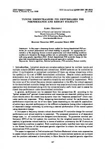
with Kp , Ti , Td , τd > 0. The parameter Kp is the proportional sensitivity constant, while Ti and Td are the time constants of the integral and derivative actions, respectively. The problem we are concerned with can be stated in precise terms as follows. Problem 2.1. Consider the feedback control architecture in Figure 1, where G(s) is the plant transfer function. Design E(s)
∣L( jωg )∣ = 1,
3.1 Steady-State requirements do not constrain Ki
CPD (s) = Kp (1 + Td s) ;
R(s)
def
e(t) = r(t) − y(t) are satisfied, and such that the crossover frequency and the phase margin of the compensated system def (loop gain transfer function) L(s) = C(s) G(s) are ωg and PM, respectively, i.e.,
First, we consider the case where the steady-state specifications do not lead to a constraint on the integral constant of the PID controller. In order to compute the parameters of the PID controller, we write G( jω ) and CPID ( jω ) in polar form as G( jω ) = ∣G( jω )∣ e j arg G( jω ) , CPID ( jω ) = M(ω ) e j ϕ (ω ) . The loop gain frequency response can be written as L( jω ) = ∣G( jω )∣ M(ω ) e j (arg G( jω )+ϕ (ω )) . If the gain crossover frequency ωg and the phase margin PM of the loop gain transfer function L(s) are assigned, (4-5) lead to ∣L( jωg )∣ = 1 and PM = π + arg L( jωg ). These equations can be written as (1) Mg = 1/ ∣G( jωg )∣ , (2) ϕg = PM − π − arg G( jωg ), def
Y (s)
def
where Mg = M(ωg ) and ϕg = ϕ (ωg ). In order to find the parameters of the controller such that (4-5) are met,
G(s)
1 + j ωg Ti − ωg2 Ti Td (6) j ωg Ti must be solved in Kp , Ti , Td > 0. In the solution to this problem there is a degree of freedom: by equating the real and imaginary parts of both sides of (6) we obtain two equations Mg e j ϕg = Kp
Fig. 1. Unity feedback control architecture. ′ (s), C (s), C (s), C′ (s)} a controller C(s) ∈ {CPID (s), CPID PI PD PD such that the steady-state requirements on the tracking error
5760
Preprints of the 18th IFAC World Congress Milano (Italy) August 28 - September 2, 2011
ωg Mg Ti cos ϕg = ωg Kp Ti ,
(7)
Kp − Kp ωg2 Ti Td
−Mg ωg Ti sin ϕg = in the three unknowns Kp , Ti and Td .
(8)
A possibility to carry out the design of the PID controller in the case of unconstrained integral constant is to exploit the remaining degree of freedom so as to satisfy some further time or frequency domain requirements. Here, we consider two ways to exploit this freedom: the first is the one where the ratio Td /Ti is chosen, so as to ensure, for example, that the zeros of the PID controller are real; the second is the one where a gain margin constraint is to be satisfied. Imposition of the ratio Td /Ti A very convenient way to exploit the degree of freedom in the solution of (6) is the impodef sition of the ratio σ = Td /Ti . This is convenient since it is an easily established fact that when Ti ≥ 4 Td , i.e., when σ −1 ≥ 4, the zeros of the PID controller are real (and coincident when σ −1 = 4), and they are complex conjugate when σ −1 < 4. In the following theorem, necessary and sufficient conditions are given for the solvability of Problem 2.1 when σ is given. Moreover, closed-form formulae are provided for the parameters of the PID controller to meet the specifications on PM, ωg and σ exactly. ˚ om et al., 1995, p. 140). Let the ratio σ = Theorem 3.1. (Astr¨ Td /Ti be assigned. Equation (6) admits solutions in Kp , Ti , Td > 0 if and only if ( π π) . (9) ϕg ∈ − , 2 2 If (9) is satsfied, the solution of (6) with σ fixed is given by Kp = Mg cos ϕg √ tan ϕg + tan2 ϕg + 4 σ Ti = 2 ωg σ Td = Ti σ
(10) (11)
def
1
,
(13)
GM ∣G( jω p )∣
ϕ p = −π − arg G( jω p ),
(14)
def
where Mp = M(ω p ) and ϕ p = ϕ (ω p ). Now Kp , Ti , Td > 0 must be determined so that (6) and 1 + j ω p Ti − ω p2 Ti Td (15) j ω p Ti are simultaneously satisfied. By equating the real and the imaginary part of (6) and (15) we obtain (7), (8) and the additional two equations Mp e j ϕ p = Kp
ω p Mp Ti cos ϕ p = ω p Kp Ti , −Mp ω p Ti sin ϕ p =
Kp − Kp ω p2 Ti Td .
Mg cos ϕg = Mp cos ϕ p (18) in the unknown ω p . For the control problem to be solvable, (18) must admit at least one strictly positive solution. Lemma 3.1. Let G(s) be a rational function in s ∈ ℂ. Then, equation (18) can be reduced to a polynomial equation in ω p . Remark 3.1. If the transfer function of the process is given by ˆ the product of a rational function G(s), and a delay e−t0 s , i.e., if −t s ˆ 0 G(s) = G(s) e , equation (18) is not polynomial in ω p , and it needs to be solved numerically. Theorem 3.2. Consider Problem 2.1 with the additional specification on the gain margin GM. Equations (6) and (15) admit solutions in Kp , Ti , Td > 0 if and only if ϕg ∈ (−π /2, π /2) and (18) admits a positive solution ω p such that { ω p < ωg ω p > ωg ωg tan ϕg > ω p tan ϕ p or ωg tan ϕg < ω p tan ϕ p (19) ω p tan ϕg > ωg tan ϕ p ω p tan ϕg < ωg tan ϕ p If ϕg ∈ (−π /2, π /2) and (19) is satisfied, the control problem admits solutions with a PID controller, whose parameters can be computed as {
Kp = Mg cos ϕg
(16) (17)
(20)
Ti =
ωg2 − ω p2 ωg ω p (ω p tan ϕg − ωg tan ϕ p )
(21)
Td =
ωg tan ϕg − ω p tan ϕ p ωg2 − ω p2
(22)
Proof: A necessary condition for the problem to admit solutions is that ω p is a solution of (18). From (7) and (8), and from (16) and (17), we obtain
(12)
Imposition of the Gain Margin Another possibility in the case of unconstrained Ki is to fix the gain margin to a certain value GM. To this end, the conditions arg L( jω p ) = −π and GM = ∣L( jω p )∣−1 on the loop gain frequency response must be satisfied by definition of gain margin and phase crossover frequency ω p . By writing again CPID ( jω ) = M(ω ) e j ϕ (ω ) , these conditions are equivalent to Mp =
From (7) and (16), we obtain the equation
−ωg Ti tan ϕg = 1 − ωg2 Ti Td ,
(23)
1 − ω p2 Ti Td .
(24) −ω p Ti tan ϕ p = By solving (23) and (24) in Ti and Td , we obtain (20-22). For Kp to be positive, it is necessary that ϕg ∈ (−π /2, π /2). Moreover, the time constants Ti and Td are positive if ωg and ω p satisfy (19). 3.2 Steady-State requirements constrain Ki Now, the Bode gain Ki = Kp /Ti is determined via the imposition of the steady-state requirements; for example, for type-0 (resp. type-1) plants, Ki is computed via the imposition of the velocity error (resp. acceleration error). As such, the factor Ki /s can be separated from C˜PID (s) = 1 + Ti s + Ti Td s2 , and viewed as part of the plant. In this way, the def ˜ part of the controller to be designed is C˜PID (s).Denote G(s) = Kp Ti s G(s), so that the loop gain transfer function can be written as ˜ ˜ jω ) and C˜PID ( jω ) in polar form L(s) = C˜PID (s) G(s). Write G( as ˜ jω ) ˜ jω )∣ e j arg G( ˜ jω ) = ∣G( , C˜PID ( jω ) = M(ω ) e j ϕ (ω ) , G( so that the loop gain frequency response can be written as ˜ jω )+ϕ (ω )) ˜ jω )∣ M(ω ) e j (arg G( L( jω ) = ∣G( . If the crossover frequency ωg and the phase margin PM of L(s) are assigned,
5761
Preprints of the 18th IFAC World Congress Milano (Italy) August 28 - September 2, 2011
√ √ 960 ( 5 2 2 + 63 ) √ + s . CPID (s) = 1+ 12 s 2160 2
the equations ∣L( jωg )∣ = 1 and PM = π + arg L( jωg ) must be satisfied. These can be written as −1 Kp ωg G( jωg ) = Mg = Ti j ωg Ki G( jωg ) ] [ Kp ϕg = PM − π − arg G( jωg ) Ti j ωg π = PM − − arg G( jωg ), 2
(25)
(26)
def
def
where Mg = M(ωg ) and ϕg = ϕ (ωg ), since Kp , Ti > 0. In order to find the parameters of the controller such that (i)-(ii) are met, equation Mg e j ϕg = 1 + j ωg Ti − Ti Td ωg2
(27)
must be solved in Ti > 0 and Td > 0. The closed-form solution to this problem is given in the following theorem. Theorem 3.3. Equation (27) admits solutions in Ti > 0 and Td > 0 if and only if 0 < ϕg < π
and
Mg cos ϕg < 1.
(28)
If (28) are satisfied, the solution of (27) is given by 1 Kp = Ki Mg sin ϕg ωg 1 Ti = Mg sin ϕg ωg 1 − Mg cos ϕg . Td = ωg Mg sin ϕg
(29) (30) (31)
Example 3.1. Consider the plant transfer function 1 G(s) = , s (s + 2)
Now we solve the same problem by imposing a gain margin equal to 3. We compute Mp and ϕ p as functions of ω p : 1 Mp = = GM∣G( j ω p )∣
∙ the acceleration error is equal to 0.005. ∙ the velocity error is equal to zero; first use the remaining degree of freedom to assign the ratio Ti /Td = 16, and then to impose a gain margin equal to 3. Consider the first problem. The acceleration error is 1 2 Ti . = 2 Kp 1 + Ti s + Ti Td s lims→0 s2 Kp Ti s2 (s + 2) ˜ Then, ea∞ = 0.005 implies Ki = Kp /Ti = 400. Define G(s) = √ Ki G(s)/s. Compute Mg = 30/Ki ∣G(30 j)∣ = 9 904/4 and ϕg = PM − π /2 − arg G(30 j) = π /4 + arctan 15. Using Theorem 3.3, the time constants of the PID controller are 1 = lims→0 s2 L(s)
√ Mg sin ϕg 1 − Mg cos ϕg 12 2 + 63 = √ , Td = . Ti = = 30 30 Mg sin ϕg 2160 5 2 The zeros of the PID controller are real since Ti is greater than √ 4 Td . From the ratio Kp /Ti = 400, we find Kp = 400 Ti = 960/ 2. The transfer function of the PID controller is
ωp
√
ω p2 + 4
; 3 ωp π ϕ p = −π − arg G( j ω p ) = − + arctan . 2 2 Using these expression, (18) can be written as
ωp
and consider the problem of determining the parameters of a PID controller that exactly achieves a phase margin of 45∘ and gain crossover frequency ωg = 30 rad/s in the two situations:
ea∞ =
Now let us consider the second problem, where the ratio Ki = Kp /Ti is not constrained. Now, the pole at the origin alone guarantees that the velocity error be equal to zero. We first −1 consider the situation where Ti /T √d = σ = 16. First, we compute Mg = 1/∣G(30 j)∣ = 30 904 and ϕg = PM − π − arg G(30 j) = π /4 − π + π /2 + arctan 15 = −π /4 + arctan 15. Using (10) we find ( π ) √ √ Kp = 30 904 cos − + arctan 15 = 480 2. 4 Moreover, a simple computation shows that tan ϕg = 7/8, so that using the results in Theorem 3.1, and in particular (11) with σ −1 = 16, we find √ √ 7 + 65 7 + 65 and Td = . Ti = 30 480 The transfer function of the PID controller in this case is ) ( √ √ 7 + 65 30 √ s . CPID (s) = 480 2 1 + + 480 (7 + 65) s
√
ω p2 + 4
( ωp ) = Mg cos ϕg , sin arctan 3 2 √ whose unique real solution is ω p = 3 Mg cos ϕg > 0. Using the for Mg and ϕg it is easily found that ω p = √ expressions √ 720 8 rad/s. Hence, √ √ √ √ π 720 8 π = − + arctan 180 8, ϕ p = − + arctan 2 2 2 √ √ which gives tan ϕ p = −1/ 180 8. It is easily verified that the conditions in Theorem 3.2 are not satisfied, since ω p > ωg but ωg tan ϕg > ω p tan ϕ p = −2. Let us consider the same problem with PM = 23π , ωg = 3 rad/s, and GM = 3. In this case, we find √ Mg = 3 13, ϕg = π6 + arctan 23 , and consequently tan ϕg = (2 + √ √ 3 3)/(2 3 − 3). Using these values in (18) yields
ωp = As such,
√
3 Mg cos ϕg =
√
9 √ (2 3 − 3). 2
√ √ π 9 (2 3 − 3) , ϕ p = − + arctan 2 8 √ √ which yields tan ϕ p = −1/ 98 (2 3 − 3). In this case, the conditions in Theorem 3.2 are satisfied, and the parameters of the PID controller can be computed in closed form as
5762
Preprints of the 18th IFAC World Congress Milano (Italy) August 28 - September 2, 2011
Kp = Mg cos ϕg =
3 √ (2 3 − 3) 2
√ ωg2 − ω p2 5−2 3 √ Ti = = ωg ω p (ω p tan ϕg − ωg tan ϕ p ) 10 + 9 3 √ ωg tan ϕg − ω p tan ϕ p 26 3 √ Td = . = ωg2 − ω p2 144 3 − 243 Since Ti < 4 Td , the zeros of the PID controller are complex conjugate.
Theorem 5.1. Equation (33) admits solutions in Kp > 0 and Td > 0 if and only if ϕg ∈ (0, π /2). If this condition is satisfied, the solution of (33) is given by Kp = Mg cos ϕg and Td = tan ϕg /ωg . When the imposition of the steady-state specifications lead ˜ to a sharp constraint on Kp , and define G(s) = Kp G(s) and ˜ jωg )∣ and ϕg = PM − C˜PD (s) = 1 + Td s, the values Mg = 1/∣G( ˜ jωg ) lead to the identity 1 + j ωg Td = Mg e j ϕg , which π − arg G( in turn leads to the two equations Mg cos ϕg = 1 and Mg sin ϕg = ωg Td , so that the problem admits solutions only if the constraint Mg cos ϕg = 1 is satisfied. In that case, Td = Mg sin ϕg /ωg .
4. PI CONTROLLERS The synthesis techniques presented in the previous sections can be adapted to the design of PI controllers for the imposition of phase margin and crossover frequency of the loop gain transfer function. This can be done, however, only when the steady-state specifications do not lead to the imposition of the Bode gain of the loop gain transfer function. The transfer function of a PI ˜ = G(s)/s, we find controller is given by (2). By defining G(s) Mg =
ωg 1 = , ˜ jωg )∣ ∣G( jωg )∣ ∣G(
˜ jωg ) = PM − π − arg G( jωg ). ϕg = PM − π − arg G( 2 To find the parameters of the PI controller, equation j Ti ωg + 1 (32) Ti must be solved in Kp > 0 and Ti > 0. Theorem 4.1. Equation (32) admits solutions in Kp > 0 and Ti > 0 if and only if ϕg ∈ (0, π /2). If this condition is satisfied, the solution of (32) is given by Kp = Mg sin ϕg /ωg and Ti = tan ϕg /ωg . Mg e j ϕg = Kp
As already observed, when the steady-state requirements lead to the imposition of the ratio Kp /Ti , the problem of assigning the phase margin and the crossover frequency of the loop gain transfer function cannot be solved in general. Indeed, if we Kp ˜ G(s) and C˜PI (s) = 1 + Ti s, the values Mg = define G(s) = Ti s ˜ jωg )∣ and ϕg = PM − π − arg G( ˜ jωg ) are such that the 1/∣G( identity 1 + j ωg Ti = Mg e j ϕg must be satisfied. The latter yields Mg cos ϕg = 1 and Mg sin ϕg = ωg Ti , which are two equations in one unknown Ti ; the first does not even depend on Ti , but only on the transfer function of the plant G(s). As such, the problem is solvable only if Mg cos ϕg = 1 is satisfied. If that constraint is satisfied, Ti = Mg sin ϕg /ωg . 5. PD CONTROLLERS As for the design of PI controllers, the synthesis techniques presented for the imposition of phase margin and crossover frequency of the loop gain transfer function can be used for PD controllers only when the steady-state specifications do not lead to the imposition of the proportional sensitivity Kp . The transfer function of a PD controller is given by (2). To find the parameters of the PD controller, the equation Mg e j ϕg = Kp (1 + j Td ωg ) must be solved in Kp > 0 and Td > 0.
(33)
6. GRAPHICAL AND APPROXIMATE SOLUTION TO THE DESIGN PROBLEM The synthesis methods developed in the previous sections are based on closed-form formulae for the computation of the parameters of the PID controller. Clearly, the strength of this approach – which provides an exact answer to the control problem design with standard steady-state and frequency domain specifications – can at first sight be also considered its weakness, because often a full knowledge of the dynamics of the plant is not available in practice. However, when this is the situation at hand, the approach presented in this paper still offers a solution to the design problem, either based on graphical considerations similar in spirit to those considered in the literature Yeung et al. (2000) (but that can be carried out on any of the standard diagrams for the frequency response), or on the approximation of the plant with a first or second order plus delay transfer function Ho et al. (1995). As already mentioned, a graphical version of the method presented in this paper can be implemented using any of the frequency domain plots usually employed in control to represent the frequency response dynamics, i.e., Bode diagrams, Nyquist diagrams or Nichols charts. This is due to the fact that the formulae used to derive the parameters of the PID controller are expressed in terms of the magnitude and the argument of the frequency response of the plant at a given crossover frequency, which is readable over any of these diagrams. Given the point of the Nyquist plot corresponding to the desired gain crossover frequency, i.e., we can estimate Mg and ϕg . These values lead to the parameters of the PID controller. This approach may be employed even in absence of graphical descriptions of the plant transfer function. Indeed, in the very same spirit of the Ziegler and Nichols method, we may “perform an experiment” on the plant by feeding it with a sinusoidal input with frequency ωg , i.e. the desired crossover frequency. From the steady-state output we can estimate G( jωg ), and hence Mg and ϕg and we can thus readily apply the proposed method. 7. SECOND ORDER PLUS DELAY APPROXIMATION Several tuning techniques proposed in the literature do not require exact knowledge of the mathematical model of the plant, but rely on its first or second order plus delay approximation, ˚ om et al. (1995). While in this paper the Ho et al. (1995); Astr¨ formulae for the parameters of the PID controller have been obtained under the assumption of exact knowledge of the transfer function of the plant, the procedure outlined can be used in conjuction with the heuristics or numerical methods based on
5763
Preprints of the 18th IFAC World Congress Milano (Italy) August 28 - September 2, 2011
these approximations. In this section we show that the formulae presented in this paper can be specialised to the case of a second order plus delay approximation of the plant dynamics. Consider the second order plus delay model K G(s) = e−T s , (1 + τ1 s)(1 + τ2 s) where τ1 , τ2 , T > 0 and K > 0. A direct calculation shows that √ (1 + ωg2 τ12 ) (1 + ωg2 τ12 ) , Mg = K ϕg = θ − π + arctan(ωg τ1 ) + arctan(ωg τ2 ), where θ = PM + ωg T , which lead to
ωg (τ1 + τ2 ) sin θ − (1 − ωg2 τ1 τ2 ) cos θ . K If the specifications are on the ratio σ = Td /Ti , the parameters of the compensator can be computed using directly (10-12), that with this particular model yield Mg cos(ϕg ) =
ωg (τ1 + τ2 ) sin θ − (1 − ωg2 τ1 τ2 ) cos θ , K (1 − ω p2 τ1 τ2 ) tan θ + ω p (τ1 + τ2 ) , Ti = (1 − ω p2 τ1 τ2 ) − ω p (τ1 + τ2 ) tan θ Td = Ti σ . If the specifications are on both the phase and gain margin (and on the gain crossover frequency), we must also compute √ (1 + ω p2 τ12 ) (1 + ω p2 τ12 ) Mp = , K ϕ p = −π + ω p T + arctan(ω p τ1 ) + arctan(ω p τ2 ), so that Kp =
ω p (τ1 +τ2 ) sin(ω p T )−(1−ω p2 τ1 τ2 ) cos(ω p T ) . GM ⋅ K Therefore, to achieve the desired margins at the desired gain crossover frequency, we need to find the roots ω p of Mp cos(ϕ p ) =
ψ (ω p ) = ω p (τ1 +τ2 ) sin(ω p T )−(1−ω p2 τ1 τ2 ) cos(ω p T ) (34) −GM ⋅ K ⋅ Mg cos(ϕg ) = 0. Notice that this time function ψ (ω p ) is not polynomial, since the transfer function of the model is not rational. The roots of this equation can be determined numerically. Of all the roots of ψ (ω p ), one satisfying the conditions of Theorem 3.2 must be determined (if no such roots exist, the problem does not admit solutions), and compute the parameters of the PID controller using (20-22). The closed-form formulae given in this paper for the parameters of the PID controller are given in finite terms. Hence, a remarkable advantage of this method is the fact that these formulae can applied to any plant approximation, even though in this section for the sake of comparison with the existing methods only the second order plus delay approximation has been considered. As such, the flexibility offered by the method presented here also extends to the case where the transfer function of the plant to be controlled is not exactly known, and necessarily guarantees a better performance when a better approximation of the plant dynamics is available. This also means that the method proposed in this paper outperformes any method constructed upon a plant approximation with a fixed structure.
8. CONCLUSIONS A unified approach has been presented that enable the parameters of PID, PI and PD controllers to be computed in finite terms given appropriate specifications expressed in terms of steadystate performance, phase/gain margins and gain crossover frequency. The synthesis tools developed in this paper eliminate the need of trial-and-error and heuristic procedures in frequency-response design, and therefore they outperform the heuristic, trial-and-error and graphic approaches proposed so far in the literature in the case of perfect knowledge of the model of the plant. When the plant model is not exactly known – as is often the case in practice – the present method can still be employed for the design of the PID controller. Indeed, the formulae delivering the controller parameters only require the magnitude and the argument of the frequency response of the plant at the desired crossover frequency. These can be obtained graphically by direct inspection over any of the Nyquist, Bode and Nichols diagrams. Alternatively, the closed-form design techniques can be used jointly with a first or second order plus delay approximation of the plant to deliver the desired values of the stability margins and crossover frequency. REFERENCES Charles L. Phillips. Analytical Bode Design of Controllers. IEEE Trans. Educ., E-28, no. 1, pp. 43–44, 1985. ˚ om, and T. Hagglund, PID Controllers: Theory, DeK.J. Astr¨ sign, and Tuning, second edition. Instrument Society of America, Research Triangle Park, NC, 1995. A. Datta, M.-T. Ho, and S.P. Bhattacharyya. Structure and Synthesis of PID Controllers. Springer, 2000. A. Ferrante, A. Lepschy, and U. Viaro. Introduzione ai Controlli Automatici. UTET Universit, 2000. G. Franklin, J.D. Powell, and A. Emami-Naeini. Feedback Control of Dynamic Systems. Prentice Hall, 2006. W.K. Ho, and C.C. Hang, and L.S. Cao, Tuning of PID Controllers Based on Gain and Phase Margin Specifications. Aut., vol. 31, no. 3, pp. 497–502, 1995. L.H. Keel and S.P. Bhattacharyya. Controller Synthesis Free of Analytical Models: Three Term Controllers. IEEE Trans. Aut. Contr., AC-53, no. 6, pp. 1353–1369, 2008. G. Marro, TFI: Insegnare ed apprendere i controlli automatici R . Zanichelli Ed., Bologna (Italy), di base con MATLAB⃝ 1998. K. Ogata. Modern Control Engineering. 2nd edn. Prentice Hall, Englewood Cliffs, NJ, 2000. S. Skogestad. Simple analytic rules for model reduction and PID controller tuning. J. Proc. Contr., vol. 13, pp. 291-309, 2003. A. Visioli, Practical PID Control. Advances in Industrial Control, Springer-Verlag, 2006. W.R. Wakeland. Bode Compensation Design. IEEE Trans. Aut. Contr., AC-21, no. 5, pp. 771–773, 1976. R. Zanasi and G. Marro, New formulae and graphics for compensator design. Proc. 1998 IEEE Int. Conf. Contr. Applic., Vol. 1, pp. 129–133, 1-4 Sept. 1998. K.S. Yeung, and K.H. Lee. A Universal Design Chart for Linear Time-Invariant Continuous-Time and Discrete-Time Compensators. IEEE Trans. Educ., E-43, no. 3, pp. 309–315, 2000. J.G. Ziegler, and N.B. Nichols, Optimum settings for automatic controllers. Trans. ASME, vol. 64, pp. 759-768, 1942.
5764