Exchange Rate Forecasting using Flexible Neural Trees Yuehui Chen1 , Lizhi Peng1 , and Ajith Abraham1,2 1
School of Information Science and Engineering Jinan University, Jinan 250022, P.R.China Email:
[email protected] 2 IITA Professorship Program, School of Computer Science and Engg. Chung-Ang University, Seoul, Republic of Korea Email:
[email protected]
Abstract. Forecasting exchange rates is an important financial problem that is receiving increasing attention especially because of its difficulty and practical applications. This paper proposes a Flexible Neural Tree (FNT) model for forecasting three major international currency exchange rates. Based on the pre-defined instruction/operator sets, a flexible neural tree model can be created and evolved. This framework allows input variables selection, over-layer connections and different activation functions for the various nodes involved. The FNT structure is developed using the Extended Compact Genetic Programming and the free parameters embedded in the neural tree are optimized by particle swarm optimization algorithm. Empirical results indicate that the proposed method is better than the conventional neural network forecasting models.
1
Introduction
Forecasting exchange rates is an important financial problem that is receiving increasing attention especially because of its difficulty and practical applications. Exchange rates are affected by many highly correlated economic, political and even psychological factors. These factors interact in a very complex fashion. Exchange rate series exhibit high volatility, complexity and noise that result from an elusive market mechanism generating daily observations [1]. Much research effort has been devoted to exploring the nonlinearity of exchange rate data and to developing specific nonlinear models to improve exchange rate forecasting, i.e., the autoregressive random variance (ARV) model [2], autoregressive conditional heteroscedasticity (ARCH) [3], self-exciting threshold autoregressive models [4]. There has been growing interest in the adoption of neural networks, fuzzy inference systems and statistical approaches for exchange rate forecasting problem [5][6][15][8][16][17]. For a recent review of neural networks based exchange rate forecasting, please consult [9]. The input dimension (i.e. the number of delayed values for prediction) and the time delay (i.e. the time interval between two time series data) are two
critical factors that affect the performance of neural networks. The selection of dimension and time delay has great significance in time series prediction. This papers proposes a Flexible Neural Tree (FNT) [10][11] for selecting the input variables and forecasting exchange rates. Based on the pre-defined instruction/operator sets, a flexible neural tree model can be created and evolved. FNT allows input variables selection, over-layer connections and different activation functions for different nodes. In our previous work, the hierarchical structure was evolved using Probabilistic Incremental Program Evolution algorithm (PIPE) with specific instructions. In this research, the hierarchical structure is evolved using the Extended Compact Genetic Programming (ECGP), a tree-structure based evolutionary algorithm. The fine tuning of the parameters encoded in the structure is accomplished using particle swarm optimization (PSO). The proposed method interleaves both optimizations. Starting with random structures and corresponding parameters, it first tries to improve the structure and then as soon as an improved structure is found, it fine tunes its parameters. It then goes back to improving the structure again and, fine tunes the structure and rules’ parameters. This loop continues until a satisfactory solution is found or a time limit is reached. The novelty of this paper is in the usage of flexible neural tree model for selecting the important inputs and/or time delays and for forecasting foreign exchange rates.
2
The Flexible Neural Tree Model
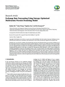
The function set F and terminal S instruction set T used for S generating a FNT model are described as S = F T = {+2 , +3 , . . . , +N } {x1 , . . . , xn }, where +i (i = 2, 3, . . . , N ) denote non-leaf nodes’ instructions and taking i arguments. x1 ,x2 ,. . .,xn are leaf nodes’ instructions and taking no other arguments. The output of a non-leaf node is calculated as a flexible neuron model (see Fig.1). From this point of view, the instruction +i is also called a flexible neuron operator with i inputs. In the creation process of neural tree, if a nonterminal instruction, i.e., +i (i = 2, 3, 4, . . . , N ) is selected, i real values are randomly generated and used for representing the connection strength between the node +i and its children. In addition, two adjustable parameters ai and bi are randomly created as flexible activation function parameters. For developing the IDS, the flexible activation −(
x−ai 2
)
bi function f (ai , bi , x) = e is used. The total excitation of +n is netn = P n j=1 wj ∗ xj , where xj (j = 1, 2, . . . , n) are the inputs to node +n . The output netn −an 2
of the node +n is then calculated by outn = f (an , bn , netn ) = e−( bn ) . The overall output of flexible neural tree can be computed from left to right by depth-first method, recursively. 2.1
Tree Structure Optimization
Finding an optimal or near-optimal neural tree is formulated as a product of evolution. In our previously studies, the Genetic Programming (GP), Proba-
+6
Output layer
x1 x2
ω1 ω2
xn
ωn
+n
f(a,b)
y
Second hidden x1 layer
x2
First hidden layer
+3
Input layer
x1
x2
+2
x3
+3
x 1 x2
+2
x3
x3
x3
x2
+3 x1 x2 x3
Fig. 1. A flexible neuron operator (left), and a typical representation of the FNT with function instruction set F = {+2 , +3 , +4 , +5 , +6 }, and terminal instruction set T = {x1 , x2 , x3 } (right)
bilistic Incremental Program Evolution (PIPE) have been explored for structure optimization of the FNT [10][11]. In this paper, the Extended Compact Genetic Programming (ECGP) [13] is employed to find an optimal or near-optimal FNT structure. ECGP is a direct extension of ECGA to the tree representation which is based on the PIPE prototype tree. In ECGA, Marginal Product Models (MPMs) are used to model the interaction among genes, represented as random variables, given a population of Genetic Algorithm individuals. MPMs are represented as measures of marginal distributions on partitions of random variables. ECGP is based on the PIPE prototype tree, and thus each node in the prototype tree is a random variable. ECGP decomposes or partitions the prototype tree into sub-trees, and the MPM factorises the joint probability of all nodes of the prototype tree, to a product of marginal distributions on a partition of its sub-trees. A greedy search heuristic is used to find an optimal MPM mode under the framework of minimum encoding inference. ECGP can represent the probability distribution for more than one node at a time. Thus, it extends PIPE in that the interactions among multiple nodes are considered. 2.2
Parameter Optimization with PSO
The Particle Swarm Optimization (PSO) conducts searches using a population of particles which correspond to individuals in evolutionary algorithm (EA). A population of particles is randomly generated initially. Each particle represents a potential solution and has a position represented by a position vector xi . A swarm of particles moves through the problem space, with the moving velocity of each particle represented by a velocity vector vi . At each time step, a function fi representing a quality measure is calculated by using xi as input. Each particle keeps track of its own best position, which is associated with the best fitness it has achieved so far in a vector pi . Furthermore, the best position among all the particles obtained so far in the population is kept track of as pg . In addition to this global version, another version of PSO keeps track of the best position among all the topological neighbors of a particle. At each time step t, by using the individual best position, pi , and the global best position, pg (t), a new velocity
for particle i is updated by vi (t + 1) = vi (t) + c1 φ1 (pi (t) − xi (t)) + c2 φ2 (pg (t) − xi (t))
(1)
where c1 and c2 are positive constant and φ1 and φ2 are uniformly distributed random number in [0,1]. The term vi is limited to the range of ±vmax . If the velocity violates this limit, it is set to its proper limit. Changing velocity this way enables the particle i to search around its individual best position, pi , and global best position, pg . Based on the updated velocities, each particle changes its position according to the following equation: xi (t + 1) = xi (t) + vi (t + 1). 2.3
(2)
Procedure of the general learning algorithm
The general learning procedure for constructing the FNT model can be described as follows. 1) Create an initial population randomly (FNT trees and its corresponding parameters); 2) Structure optimization is achieved by using the ECGP algorithm; 3) If a better structure is found, then go to step 4), otherwise go to step 2); 4) Parameter optimization is achieved by the PSO algorithm as described in subsection 2. In this stage, the architecture of FNT model is fixed, and it is the best tree developed during the end of run of the structure search. The parameters (weights and flexible activation function parameters) encoded in the best tree formulate a particle. 5) If the maximum number of local search is reached, or no better parameter vector is found for a significantly long time then go to step 6); otherwise go to step 4); 6) If satisfactory solution is found, then the algorithm is stopped; otherwise go to step 2).
3 3.1
Exchange Rates Forecasting Using FNT Paradigms The Data Set
We used three different datasets in our forecast performance analysis. The data used are daily forex exchange rates obtained from the Pacific Exchange Rate Service [14], provided by Professor Werner Antweiler, University of British Columbia, Vancouver, Canada. The data comprises of the US dollar exchange rate against Euros, Great Britain Pound (GBP) and Japanese Yen (JPY). We used the daily data from 1 January 2000 to 31 October 2002 as training data set, and the data from 1 November 2002 to 31 December 2002 as evaluation test set or out-of-sample datasets (partial data sets excluding holidays), which are used to evaluate the good or bad performance of the predictions, based on evaluation measurements.
The forecasting evaluation criteria used is the normalized mean squared error (NMSE), PN t=1 N M SE = PN
(yt − yˆt )2
t=1 (yt
− y¯t )2
=
N 1 1 X (yt − yˆt )2 , σ 2 N t=1
(3)
where yt and yˆt are the actual and predicted values, σ 2 is the estimated variance of the data and y¯t the mean. The ability to forecast movement direction or turning points can be measured by a statistic developed by Yao and Tan [12]. Directional change statistics (Dstat) can be expressed as Dstat =
N 1 X at × 100%, N t=1
(4)
where at = 1 if (yt+1 − yt )(ˆ yt+1 − yˆt ) ≥ 0, and at = 0 otherwise. 3.2
Feature/Input Selection with FNT
It is often a difficult task to select important variables for a forecasting or classification problem, especially when the feature space is large. A fully connected NN classifier usually cannot do this. In the perspective of FNT framework, the nature of model construction procedure allows the FNT to identify important input features in building an IDS that is computationally efficient and effective. The mechanisms of input selection in the FNT constructing procedure are as follows. (1) Initially the input variables are selected to formulate the FNT model with same probabilities; (2) The variables which have more contribution to the objective function will be enhanced and have high opportunity to survive in the next generation by a evolutionary procedure; (3) The evolutionary operators i.e., crossover and mutation, provide a input selection method by which the FNT should select appropriate variables automatically. 3.3
Experimental Results
For simulation, the five-day-ahead data sets are prepared for constructing FNT models. A FNT model was constructed using the training data and then the model was used on the test dataSset. The instruction sets used to create an S optimal FNT forecaster is S = F T = {+2 , +3 } {x1 , x2 , x3 , x4 , x5 }. Where xi (i = 1, 2, 3, 4, 5) denotes the 5 input variables of the forecasting model. The optimal FNTs evolved for three major internationally traded currencies: British pounds, euros and Japanese yen are shown in Figure 2. It should be noted that the important features for constructing the FNT model were formulated in accordance with the procedure mentioned in the previous section. For comparison purpose, the forecast performances of a traditional multilayer feed-forward network (MLFN) model and an adaptive smoothing neural network (ASNN) model are also shown in Tables 1 and 2. The actual daily
+2
+3
+2
x0 x4
+2
x4
+3
+3
x3 x4
x1
x0
+3
+3
+3
+2
x4
x2
+2
+2
x0 x1 x2 x1 x4 x3 x4
x0
+3
+2 x2
x4 x1 x3
+2
+3
x4
+2
x1 x3 x1
x0 x1 x3
Fig. 2. The evolved FNT trees for forecasting euros (left), British pounds (middle) and Japanese yen (right). Table 1. Forecast performance evaluation for the three exchange rates (NMSE for testing) Exchange rate
euros
British pounds
Japanese yen
MLFN [15]
0.5534
0.2137
0.2737
ASNN [15]
0.1254
0.0896
0.1328
FNT (This paper)
0.0180
0.0142
0.0084
Table 2. Forecast performance evaluation for the three exchange rates (Dstat for testing) Exchange rate
euros
British pounds
MLFN [15]
57.5%
55.0%
Japanese yen 52.5%
ASNN [15]
72.5%
77.5%
67.5%
FNT (This paper)
81.0
84.5%
74.5%
exchange rates and the predicted ones for three major internationally traded currencies are shown in Figures 3, 4 and 5. From Tables 1 and 2, it is observed that the proposed FNT forecasting models are better than other neural networks models for three major internationally traded currencies.
4
Conclusions
In this paper, we presented a Flexible Neural Tree (FNT) model for forecasting three major international currency exchange rates. We have demonstrated that the FNT forecasting model may provide better forecasts than the traditional MLFN forecasting model and the ASNN forecasting model. The comparative evaluation is based on a variety of statistical measures such as NMSE and Dstat . Our experimental analyses reveal that the NMSE and Dstat for three currencies
Training
Testing
1 0.9 0.8
Target and forecast
0.7 0.6 0.5 0.4 0.3 Target Forecast
0.2 0.1 0
0
100
200
300
400
500
600
700
800
s
Time serie
Fig. 3. The actual exchange rate and predicted ones for training and testing data set (euros) Training
Testing
1 0.9 0.8
Target and forecast
0.7 0.6 0.5 0.4 Target Forecast
0.3 0.2 0.1 0
0
100
200
300
400
500
600
700
800
s
Time serie
Fig. 4. The actual exchange rate and predicted ones for training dan testing data set (British pounds) Training
Testing
1 0.9
Target Forecast
Target and forecast
0.8 0.7 0.6 0.5 0.4 0.3 0.2 0.1 0
0
100
200
300
400
500
600
700
800
Time serie s
Fig. 5. The actual exchange rate and predicted ones for training dan testing data set (Japanese yen)
using the FNT model are significantly better than those using the MLFN model and the ASNN model. This implies that the proposed FNT model can be used as a feasible solution for exchange rate forecasting.
Acknowledgment This research was partially supported the Natural Science Foundation of China under contract number 60573065, and The Provincial Science and Technology Development Program of Shandong under contract number SDSP2004-0720-03.
References 1. P. Theodossiou, ”The stochastic properties of major Canadian exchange rates”. The Financial Review 29(2):193-221, 1994. 2. M. K. P. So, K. Lam and W. K. Li., ”Forecasting exchange rate volatility using autoregressive random variance model”, Applied Financial Economics, 9:583-591, 1999. 3. D. A. Hsieh. ”Modeling heteroscedasticity in daily foreign-exchange rates”, Journal of Business and Economic Statistics, 7:307C317, 1989. 4. D. Chappel, J. Padmore, P. Mistry and C. Ellis. ”A threshold model for French franc/Deutsch mark exchange rate”, Journal of Forecasting, 15:155-164, 1996. 5. A. N. Refenes. ”Constructive learning and its application to currency exchange rate forecasting”, In Neural Networks in Finance and Investing: Using Artificial Intelligence to Improve Real-World Performance, eds. R. R. Trippi and E. Turban (Probus Publishing Company, Chicago), pp. 777-805, 1993. 6. A. N. Refenes,M. Azema-Barac, L. Chen and S. A. Karoussos. ”Currency exchange rate prediction and neural network design strategies”, Neural Computing and Application, 1:46-58, 1993. 7. L.Yu, S. Wang, and K. K. Lai. ”Adaptive Smoothing Neural Networks in Foreign Exchange Rate Forecasting”, V.S. Sunderam et al. (Eds.): ICCS 2005, LNCS 3516, pp. 523-530, 2005. 8. L.Yu, S. Wang, and K. K. Lai. ”A novel nonlinear ensemble forecasting model incorporating GLAR andANN for foreign exchange rates”, Computers & Operations Research 32:2523-2541, 2005. 9. W. Wang, K.K.Lai, Y.Nakamori, S.Wang. ”Forecasting Foreign Exchange Rates with Artificial Neural Networks: A Review”. International Journal of Information Technology & Decision Making, 3(1):145-165, 2004. 10. Y. Chen, B. Yang and J. Dong, ”Nonlinear System Modeling via Optimal Design of Neural Trees”, International Journal of Neural Systems, 14(2):125-137, 2004. 11. Y. Chen, B. Yang, J. Dong, and A. Abraham, ”Time-series Forecasting using Flexible Neural Tree Model”, Information Science, Vol.174, Issues 3/4, pp.219-235, 2005. 12. J.T. Yao, C.L. Tan. ”A case study on using neural networks to perform technical forecasting of forex”, Neurocomputing, 34:79-98, 2000. 13. K. Sastry and D. E. Goldberg. ”Probabilistic model building and competent genetic programming”, In R. L. Riolo and B. Worzel, editors, Genetic Programming Theory and Practise, chapter 13, pp. 205-220. Kluwer, 2003. 14. http://fx.sauder.ubc.ca/
15. L. Yu, S. Wang, and K. K. Lai, ”Adaptive Smoothing Neural Networks in Foreign Exchange Rate Forecasting”, V.S. Sunderam et al. (Eds.): ICCS 2005, LNCS 3516, 523-530, 2005. 16. A. Abraham, Analysis of Hybrid Soft and Hard Computing Techniques for Forex Monitoring Systems, IEEE International Conference on Fuzzy Systems (IEEE FUZZ’02), 2002 IEEE World Congress on Computational Intelligence, ISBN 0780372808, IEEE Press pp. 1616 -1622, 2002. 17. A. Abraham, M. Chowdury and S. Petrovic-Lazerevic, Australian Forex Market Analysis Using Connectionist Models, Management Journal of Management Theory and Practice, No. 29, VIII, pp. 18-22, 2003.