Existence, uniqueness and efficiency of equilibrium in hedonic markets with multidimensional types. Ivar Ekeland Canada Research Chair in Mathematical Economics University of British Columbia
[email protected] April 15, 2005 We prove the existence and uniqueness of equilibrium in hedonic markets, when consumers and suppliers have reservation utilities and the utility functions are separable with respect to price. Consumers and suppliers are restricted to trading one or zero unit of an indivisible good characterized by a multidimensional quality, so that each trade matches a seller with a buyer. This is part of an ongoing research program with Jim Heckman, Lars Nesheim and Rosa Matzkin. I am particulary grateful to Jim Heckman for explaining hedonic models to me, discussing preliminary versions of the paper and sharing his economic insight. I am thankful to Pierre-Andre Chiappori, Lars Nesheim, Michael Peter, Art Shneyerov and Jean-Francois Jacques for valuable discussions leading to substantial improvement, and to all the participants in the May 2004 workshop on Mathematical Structures in Economic Theory and Econometrics, where this paper was presented. I also wish to thank Simon Ljusberg for a careful reading of the manuscript.
1
Introduction.
1.1
Main results.
In this paper, we show the existence and uniqueness of equilibrium in a hedonic market, and we give uniqueness results. The main features of our model are as follows: • There is a single, indivisible, good in the market, and it comes in different qualities z • Consumers and producers are price-takers and utility-maximizers. They are characterized by the values of some variables; each set of values is called a (multidimensional) type. 1
• Consumers buy at most one unit of the good, and they buy none if their reservation utility is not met; producers supply at most one unit of the good, and they supply none if their reservation utility is not met. In other words, agents always have the option of staying out of the market. • The utilities of consumers and of producers are quasi-linear with respect to price: the utility consumers with type x derive from buying one unit of quality z at price p (z) is u (x, z) − p (z), and the utility producers with type y derive from selling one unit of quality z at price p (z) is p (z) − v (y, z) Our results are valid in the discrete case and in the continuous case. We show that there is a (nonlinear) price system p (z) such that, for every quality z, the number (or the aggregate mass) of consumers who demand z is equal to the number (or the aggregate mass) of suppliers who produce z. In addition, agents who are staying out of the market are doing so because by entering they would lower their utility. In other words this price system exactly matches a subset of consumers with a subset of producers, and the remaining consumers or producers are priced out of the market. This is called an equilibrium price, and the resulting allocation of qualities is called an equilibrium allocation. An example is given in section 4.4, and the reader may proceed there directly. We should stress, however, that we prove existence in full generality, beyond the one-dimensional situation described in that example. Every price system p (z) creates a matching between consumers and producers: for every unit traded, there is a pair consisting of a consumer who buys it and a producer who sells it. When summing their utilities, the price of the traded item cancels out, so that the resulting utility of the pair is independent of the price system. Unmatched consumers and producers (singles) get their reservation utility. It is then meaningful to take the social planner’s point of view, and to ask for a matching between consumers and producers which will maximize aggregate utility, where the utility of matched pairs is the maximum utility they can get by trading, and the utility of unmatched agents is their reservation utility. We will show that the solution of this problem coincides with the equilibrium matching. This implies that every equilibrium is efficient. An interesting feature of equilibrium pricing is that, even tough all technologically feasible qualities are priced, not all of them will be traded in equilibrium. For each non-traded quality, there is a non-empty bid-ask range: all prices which fall within that range are equilibrium prices, that is, they will 2
not lure customers or suppliers away from traded qualities. This means that equilibrium prices cannot be uniquely defined on non-traded qualities. On the other hand, they are uniquely defined on traded qualities. There is a corresponding degree of uniqueness for the equilibrium allocation. The main drawback of our model is the assumption that utilities are quasi-linear. It is quite a restriction, from the economic point of view, since it means that the marginal utility of money is constant, but our proof seems to require it in an essential way. On the other hand, it also enables us to prove some uniqueness results, which are probably not to be expected in the more general case.
1.2
The literature.
This paper inherits from two traditions in economics. On the one hand, is can be seen as a contribution to the research program on hedonic pricing that was outlined by Shervin Rosen in his seminal paper [16]. The idea of defining a good as a bundle of attributes (originating perhaps with Houthakker [9], and developed by Lancaster [11], Becker [1] and Muth [12]), provides a systematic framework for the economic analysis of the supply and demand for quality. The main direction of investigation, however, has been towards econometric issues, such as the construction of price indices net of changes in quality; see for instance the seminal work of Court [3] and the book [8]). The identification of hedonic models raises specific questions which have been first discussed by Rosen [16], and most recently by Ekeland, Heckman and Nesheim [4]. Theoretical question, such as the existence and characterization of equilibria, have attracted less attention. The papers by Rosen [16] and later Mussa and Rosen [14] study the one-dimensional situation, that is, the case when agents are fully characterized by the value of a single parameter. The multidimensional situation has been investigated by Rochet and Choné [15], but it deals with monopoly pricing. The issue of equilibrium pricing in the multidimensional situation, had to my knowledge not been adressed up to now (nor, for that matter, has the issue of oligopoly pricing). One of Rosen’s main achievement has been to recognize hedonic pricing as nonlinear, against the prevailing tradition in econometric usage. As noted in [16], a buyer can force prices to be linear with respect to quality if certain types of arbitrage are allowed. In the present paper, buyers and sellers are restricted to trading one unit of a single quality, and there is no second-hand market, so this kind of arbitrage is unavailable, and prices will be inherently nonlinear. This would not be the case if consumers and producers were allowed to buy and sell several qualities simultaneously. On the other hand, this paper also belongs to the tradition of assignment 3
problems. This tradition has several strands, one of which originates with Koopmans and Beckmann [10], and the other with Shapley and Shubik [17]. We refer to the papers by Gretzki, Ostroy and Zame [6] and [7], and to [13] for more recent work. In this literature, producers are not free to choose the quality they sell: each quality is associated with a single producer, who can produce that one and not any other one. The Shapley-Shubik model, for instance, describes a market for houses. There are a certain number of sellers, each one is endowed with a house, and a certain number of buyers. No seller can sell a house other than his own, but a buyer can buy any house. This is in contrast with the situation in the present paper, where both buyers and sellers are free to choose the quality they buy or sell.
1.3
Structure of the paper
Section 2 describes the mathematical model and the basic assumptions. As we mentioned earlier, we do not require that the distribution of types be continuous, nor that the number of consumers equals the number of producers. Mathematically speaking, there is a positive measure µ on the set of consumer types X, and a measure ν on the set of producer types Y , both µ and ν can have atoms, and typically µ (X) 6= ν (Y ). These features, although very appealing from the point of view of economic modelling, introduce great complications in the mathematical treatment. In earlier work [5], the author has given a streamlined proof in the particular case when µ and ν are nonatomic, µ (X) = ν (Y ) and an additional sorting assumption on utilities is satisfied (extending to multidimensional types the classical Spence-Mirrlees single-crossing assumption), so that all agents with the same type do the same thing. Beside the fact that it does not apply when X or Y are finite, such a model does not capture one of the essential role of prices, which serve not only to match consumers and producers which enter the market (there must necessarily be an equal number of both) but also to keep out of the market enough agents so that matching becomes possible. The latter function is an essential focus of the present paper. In our model, there is a single indivisible good, consumers are restricted to buying one or zero unit, and producers are restricted to supply one or zero unit. The price is a nonlinear function p (z) of the quality z. It is an equilibrium price if the market for every quality clears. This implies that the number of consumers who trade is equal to the number of suppliers who trade. The remaining, non-trading, agents, are kept out of the market by the price system, which is either too high (for consumers) or too low (for producer) to allow them to make more than their reservation utility. It is important to note that in equilibrium consumers (or producers) which 4
have the same type may not be doing the same thing. This will typically occur when utility maximisation does not result in a single quality being selected. To be precise, given an equilibrium price p (z), consumers of type x maximize u (x, z) − p (z) with respect to z. But there is no reason why there should be a unique optimal quality: even if we assumed u (x, z) to be strictly concave with respect to z, the price p (z) typically is nonlinear with respect to z, and no conclusion can be derived about uniqueness. If p (z) is an equilibrium price, and if there is a non-trivial subset D (x) ⊂ Z such that any z ∈ D (x) is a utility mazimizer for x, there will be a certain equilibrium probability Pxα on D (x). This means that, given A ⊂ D (x) , the number Pxα [A] ∈ [0, 1] is the proportion of agents of type x whose demands lie in A. Similarly, there will be an equilibrium probability Pyβ for every producer y, and the resulting demand and supply for every quality z will balance out. A formal definition is given in section 3. In other words, in equilibrium, we cannot tell which agent of a given type does what, but we can tell how many of them do this or that. The main results of the paper, together with the definition of equilibrium, are stated in section 3: equilibria exist, equilibrium prices are not unique, there is a unique equilibrium allocation, and it is efficient (Pareto optimal). Proofs are deferred to Appendices C and D. These proofs combine two mathematical ingredients, the Hahn-Banach separation theorem on the one hand, and duality techniques which extend the classical Fenchel duality for convex functions, and which have been developed in the context of optimal transportation (see [18] for a recent survey). Everything relies in studying a certain optimization problem (30), which is novel. Section 4 gives additional assumptions which ensure that all agents of the same type do the same thing in equilibrium: µ and ν should be non-atomic, and conditions (8) and (9) should be satisfied. These conditions extend to multidimensional types the classical single-crossing assumption of Spence and Mirrlees. The resulting equilibria are called pure, in reference to pure and mixed equilibria in game theory. Note however that, even in this case, one cannot fully determine the behaviour of agents in equilibrium: if consumers of type x are indifferent between entering the market or not (either decision giving them their reservation utility), then, even with these additional assumptions, we cannot say which ones will stay out and which ones will come in. The equilibrium relations will only determine the proportion of each. Subsection 4.4 describes an explicit example. It is strictly one-dimensional (types and qualities are real numbers), which makes calculations possible, and a complete description of the equilibrium is provided. Unfortunately, the method used does not extend to multidimensional types. Appendix A gives the mathematical results on u-convex and v-concave 5
analysis which will be in constant use in the text. Appendix B gives general mathematical notations, and references about Radon measures. Appendices C and D contain proofs.
2 2.1
The model. Standing assumptions.
Let X ⊂ Rd1 , Y ⊂ Rd2 , and Z0 ⊂ Rd3 be compact subsets. We are given non-negative finite measures µ on X and ν on Y. They are allowed to have point masses. Typically, we will have µ (X) 6= ν (Y ). Let Ω1 be a neighbourhood of X × Z0 in Rd1 +d3 , and Ω2 be a neighbourd +d hood of Y × Z0 in R 2 3 . We are given continuous functions u : Ω1 → R and v : Ω2 → R. It is assumed that u is differentiable with respect to x, and that the derivative: ¶ µ ∂u ∂u Dx u = , ..., ∂x1 ∂xd1 is continuous with respect to (x, z). Similarly it is assumed that v is differentiable with respect to y, and that the derivative Dy v is continuous with respect to (y, z). Note that X, Y and/or Z0 are allowed to be finite. If X is finite, the assumption on u is satisfied. If Y is finite, the assumption on v is satisfied.
2.2
Bid and ask prices
We are describing the market for a quality good: it is indivisible, and units differ by their characteristics (z1 , ..., zd3 ) ∈ Z0 . The bundle z = (z1 , ..., zd3 ) will be referred to as a (multidimensional) quality. So Z0 is the set of all technologically feasible qualities; it is to be expected that they will not all be traded in equilibrium. Points in X represent consumer types, points in Y represent producer types. If X is finite, then µ (x) is the number of consumers of type x. If Y is finite, then ν (y) is the number of producers of type y. If X is infinite, then µ is the distribution of types in the consumer population, and the same interpretation holds for (Y, ν). Each consumer buys zero or one unit, and each supplier sells zero or one unit. There is no second-hand trade. For the time being, we define a price system to be a continuous map p : Z0 → R. This definition will be modified in a moment, as the set Z0 will 6
be extended to a larger set Z. Typically, pricing is nonlinear with respect to the characteristics. Once the price system is announced, agents make their decisions according to the following rules: • Consumers of type x maximize u (x, z) − p (z) over Z0 . If the value of that maximum is strictly positive, the consumer enters the market and buys one unit of the maximizing quality z. If there are several maximizing qualities, he is indifferent between them, and the way he chooses which one to buy is not specified at this stage. If the value of the maximum is 0, he is indifferent between staying out of the market, and entering it to buy one unit of the maximizing quality. Again, the way he chooses is not specified at this stage. • Producers of type y maximize p (z)−v (y, z) over Z0 . If the value of that maximum is strictly positive, the producer enters the market and sells one unit of the maximizing quality z. If there are several maximizing qualities, he is indifferent between them. If the value of the maximum is 0, he is indifferent between staying out of the market, and entering it to sell one unit of the maximizing quality. To model this procedure by a straigthforward maximization, we introduce two extra points ∅d ∈ / Z0 and ∅s ∈ / Z0 , with ∅d 6= ∅s , and we extend utilities and prices as follows: p (∅d ) = u (x, ∅d ) = 0 ∀x ∈ X p (∅s ) = v (y, ∅s ) = 0 ∀y ∈ Y u (x, ∅s ) = −1 , v (y, ∅d ) = 1
(1) (2) (3)
The set of possible decisions for agents is now Z = Z0 ∪ {∅d } ∪ {∅s } so that: max {u (x, z) − p (z) | z ∈ Z} ≥ u (x, ∅d ) − p (∅d ) = 0 max {p (z) − v (y, z) | z ∈ Z} ≥ p (∅s ) − v (y, ∅s ) = 0 and the procedure we just described amounts to maximizing over Z instead of Z0 . The relations (1) to (3) imply that consumers will never choose ∅s (it is always better to choose ∅d ), and producers will never choose ∅d (it is always better to choose ∅s ). So our model does capture the intended behaviour. Note that we have normalized reservation utilities to 0. This does not cause any loss of generality. The behaviour of consumers, for instance, is 7
fully specified by u (x, z) and u¯ (x), the latter being the reservation utility, and we get the same behaviour by replacing u (x, z) by u (x, z) − u¯ (x) and u¯ (x) by 0, the only restriction being that we would require u¯ to be C 1 , to preserve the regularity properties of u. Normalizing reservation utilities to 0, we find that u (x, z) is the bid price for quality z by consumers of type x, that is, the highest price that they are willing to pay for that quality. Similarly, v (y, z) is the asking price for quality z by producers of type y , that is, the lowest price they are willing to accept for supplying that quality. For a given quality z ∈ Z, it is natural to consider the highest bid price from consumers and the lowest ask price from producers: Definition 1 The highest bid price b : Z → R is given by: b (z) = max u (x, z) x
and the lowest ask price a : Z → R is given by: a (z) = min v (y, z) y
Note that b (∅d ) = a (∅s ) = 0 and that a (∅d ) = −b (∅s ) = 1. It follows from their definitions that b is u-convex and a is v-concave. More precisely, we have b (z) = 0x and a (z) = 0y where 0x and 0y denote the maps x → 0 and y → 0 on X and Y . Conversely, we have 0 = maxz {u (x, z) − b (z)} and 0 = minz {v (y, z) − a (z)}, so that b (x) = 0 and a (y) = 0. Note that if the price system is such that p (z) > b (z) for some quality z, then there will be no buyers for this quality, and so it cannot be traded at that price. Similarly, if p (z) < a (z), then there will be no sellers for this quality, and it cannot be traded at that price. The following is obvious: Proposition 2 (No-trade equilibrium) If a (z) > b (z) everywhere, then all consumers and all producers stay out of the market.
2.3
Demand and supply
From now on, a price system will be a continuous map p : Z → R such that p (∅d ) = p (∅s ) = 0. Given a price system p, the map p : Z → R is continuous and the set Z is compact, so that the functions u (x, z) − p (z) and p (z) − v (y, z) attain their maximum on Z. 8
Definition 3 Given a price system p, we define: D (x) = arg max {u (x, z) − p (z) | z ∈ Z} S (y) = arg min {v (y, z) − p (z) | z ∈ Z} Both are compact and non-empty subsets of Z. We shall refer to D (x) as the demand of type x consumers, and to S (y) as the supply of type y producers. It follows from the definitions that if a consumer of type x is out of the market, then we must have ∅d ∈ D (x) . If there is no other point in D (x), then all consumers of the same type stay out of the market. If, on the other hand, D (x) contains some point z ∈ Z0 , then all consumers of type x are indifferent between staying out or buying quality z, and we may expect that some of them actually buy quality z instead of staying out. This remark will be at the core of our equilibrium analysis. Of course, the same observation is valid for producers. The following result clarifies the relation between D (x) and S (y) on the one hand, and the sub- and supergradients ∂p (x) and ∂p (y) on the other. Recall that: p (x) = max {u (x, z) − p (z) | z ∈ Z} p (y) = min {v (y, z) − p (z) | z ∈ Z}
Proposition 4 We have D (x) ⊂ ∂p (x) and S (y) ⊂ ∂p (y). More precisely: ª © D (x) = z ∈ ∂p (x) | p (z) = p (z) © ª S (y) = z ∈ ∂p (y) | p (z) = p (z)
Proof. The point x ∈ X being fixed, consider the functions ϕ : Z → R and ψ : Z → R defined by ϕ (z) = u (x, z)−p (z) and ψ (z) = u (x, z)−p (z). The subgradient ∂p (x) is the set of points z where ψ attains its maximum (see section ), while D (x) is the set of points z where ϕ attains its maximum. But ψ ≥ ϕ and max ψ = max ϕ. The result follows.
Definition 5 Given a price system p (z), consumers of type x are inactive if p (x) < 0, so that D (x) = {∅d }, and they are active if p (x) > 0, so that {∅d } ∈ / D (x). They are indifferent if p (x) = 0, so that D (x) ⊃ {∅d } ∪ {z} for some z ∈ Z0 . Similarly, producers of type y are inactive, active or indifferent according to whether p (y) is positive, negative or zero.
9
2.4
Admissible price systems
We have seen that, if a (z) > b (z) everywhere, there is a no-trade equilibrium. We are concerned with the more interesting case when a (z) ≤ b (z) for some z. Definition 6 Quality z ∈ Z is marketable if a (z) ≤ b (z). The set of marketable qualities will be denoted by Z1 : Z1 = {z ∈ Z | a (z) ≤ b (z)} = {z ∈ Z | ∃ x , ∃ y : v (y, z) ≤ u (x, z)} Note that staying out is not a marketable option: a (∅d ) > b (∅d ) and a (∅s ) > b (∅s ). As mentioned earlier, this means that consumers will never choose ∅s and that suppliers will never choose ∅d . We have therefore the inclusions: Z1 ⊂ Z0 Ã Z
If a quality z is not marketable, one will never be able to find a buyer/seller pair that trade z. If a quality z is marketable, there is no sense in setting its price to be higher than b (z) (there would be no buyers), or lower than a (z) (there would be no sellers). Hence: Definition 7 A price system p : Z → R will be called admissible if: ∀z ∈ Z1 , a (z) ≤ p (z) ≤ b (z)
Let p be an admissible price system, so that a (z) ≤ p (z) ≤ b (z). Recall that p (x) is the indirect utility of type x consumers, and that −p (y) is the indirect utility of type y producers. Taking conjugates, we get: ∀x ∈ X, 0 ≤ p (x) ∀y ∈ Y,
0 ≥ p (y)
which means that all consumers and producers achieve at least their reservation utility.
3 3.1
Equilibrium Demand distribution and supply distribution
Assume a price system p : Z → R is given. Let D (x) and S (y) be the associated demand and supply. Recall. that their graphs are compact sets. We refer to Appendix B for notations and definitions concerning Radon measures and probabilities. Given a finite positive measure αX×Y on 10
Definition 8 A demand distribution associated with p is a positive measure αX×Z on X × Z such that: • αX×Z is carried by the graph of D • its marginal αX is equal to µ Similarly, a supply distribution associated with p is a positive measure βY ×Z on Y × Z such that: • βY ×Z is carried by the graph of S • its marginal βY is equal to ν The conditional probabilities Pxα and Pyβ then are carried by D (x) and S (y) respectively. Given A ⊂ Z, the numbers Pxα [A] and Pyβ [A] are readily interpreted as the probability that consumers of type x demand some z ∈ A and the probability that producers of type y supply some z ∈ A. If S (x) is a singleton, so that the supply of type y producers is uniquely defined, then Pyβ reduces to a Dirac mass: S (y) = {s (y)} =⇒ Pyβ = δs(y) and similarly for consumers.
3.2
Definition of equilibrium
Definition 9 An equilibrium is a triplet (p, αX×Z , βY ×Z ), where p is an admissible price system and αX×Z and βY ×Z are demand and supply distributions associated with p, such that: αZ0 = βZ0 By αZ0 and βZ0 we denote the marginals of αX×Z and βY ×Z on Z0 . Let us write down explicitly all the conditions on (p, α, β) implied by this definition: 1. p : Z → R is continuous, and p (z) ∈ [a (z) , b (z)] whenever a (z) ≤ b (z) 2. the marginal αX is equal to µ 3. the conditional probability Pxα is carried by D (x) 4. the marginal βY is equal to ν 11
5. the conditional probability Pyβ is carried by S (y) 6. the marginals αZ and βZ coincide on Z0 : αZ [A] = βZ [A]
∀A ⊂ Z0
The interpretation is as follows. Given p, consumers of type x maximize their utility, thereby defining their individual demand set D (x). If that set is a singleton, D (x) = {d (x)}, the probability Pxα must be the Dirac mass carried by d (x), and all consumers of type x do the same thing: they stay out of the market if d (x) = ∅d , and they buy z ∈ Z0 if d (x) = z. If D (x) contains several points, then consumers of type x are indifferent among these alternatives, and they all do different things. For any Borel subset A ⊂ D (x), the probability Pxα [A] gives us the proportion of consumers of type x who choose some z ∈ A in equilibrium. Similar considerations hold for suppliers. Condition 6 just states that markets clear in equilibrium: for every quality z ∈ Z0 , the number (or the aggregate mass) of buyers equals the number (or the aggregate mass) of suppliers. Note that this number (or this mass) might be zero, meaning that this particular quality is not traded. This will happen, for instance, if a (z) > b (z), so that quality z is not marketable. It follows that, in equilibrium, demand and supply are carried by Z1 , the set of marketable qualities: αZ [Z1 ] = αZ [Z0 ] = βZ [Z0 ] = βZ [Z1 ] The number (or the aggregate mass) of consumers who stay out of the market is αZ ({∅d }), and the number (or the aggregate mass) of producers who stay out of the market is βZ ({∅s }). As we mentioned several times before, we must have αZ ({∅s }) = 0 and βZ ({∅d }) = 0.
3.3
Main results
We begin by an existence result: Theorem 10 (Existence) Under the standing assumptions, there is an equilibrium. As noted above, if the set Z1 of marketable qualities is empty, there is an equilibrium, namely the no-trade equilibrium, and it is unique. From now on we assume Z1 6= ∅. The Existence Theorem will be proved in section C. There is no uniqueness of equilibrium prices. For instance, if a quality z ∈ Z0 is non-marketable, its price p (z) can be specified arbitrarily. More generally, in section C we will prove the following (see Proposition 37): 12
Theorem 11 (Non-uniqueness of equilibrium prices) The set of all equilibrium prices p is convex and non-empty. If p : Z → R is an equilibrium price, then so is every q : Z → R which is admissible, continuous, and satisfies: p (z) ≤ q (z) ≤ p (z) ∀z ∈ Z (4)
For α- and β-almost every quality z which is traded in equilibrium, we have p (z) = p (z) = p (z).
Note that q is also required to be admissible, so that in addition to (4) it has to satisfy the inequality: a≤q≤b (5)
The economic interpretation is as follows. If (p, αX×Z , βY ×Z ) is an equilibrium, there will be qualities z which are marketable, but which are not traded in equilibrium, because every supplier type y and every consumer type x prefers some other quality, which means that the price p (z) is too low to interest suppliers, and too high to interest consumers. Formulas (4) and (5) give the range of prices for which this situation will persist. As long as the price p (z) stays in the open interval © ª © ª ] max a (z) , p (z) , min b (z) , p (z) [
the quality z will not be traded. In other words, the price of non-traded qualities can be changed, within a certain range, without affecting αX×Z or βY ×Z , that is, the equilibrium distribution of consumers and suppliers. This is the major source of non-uniqueness in equilibrium prices. On the other hand, if a quality z is traded in equilibrium, one cannot change the price p (z) without affecting αX×Z and βY ×Z , that is, without destroying the given equilibrium. The equilibrium price p is not unique, but the following result shows that the demand and supply maps D (x) and S (y) almost are: ¡ ¢ 1 1 Theorem 12 (Uniqueness of equilibrium allocations) Let p , α , β 1 X×Z Y ×Z ¢ ¡ 2 , βY2 ×Z be two equilibria. Denote by D1 (x) , D2 (x) and S1 (y) , S2 (y) and p2 , αX×Z the corresponding demand and supply maps. Denote by Px1 , Py1 and Px2 , Py2 the corresponding conditional probabilities of demand and supply. Then: Px2 [D1 (x)] = Px1 [D1 (x)] = 1 for µ-a.e. x Py2 [S1 (y)] = Py1 [S1 (y)] = 1 for ν-a.e. y Corollary 13 If the demand of consumers of type x is single-valued in the first equilibrium, D1 (x) = {d1 (x)}, then d1 (x) ∈ D2 (x). If their demand is single-valued in the second equilibrium as well, then d1 (x) = d2 (x). 13
Proof. We have Px2 [d1 (x)] = 1 = Px2 [D2 (x)]. So d1 (x) must belong to D2 (x), and the remainder must have zero probability: Px2 [D2 (x) Â {d1 (x)}] = 0 ¡ ¢ ¡ ¢ 1 2 Corollary 14 Let p1 , αX×Z , βY1 ×Z and p2 , αX×Z , βY2 ×Z be two equilibria. If consumers of type x are inactive in the first equilibrium, they cannot be active in the second. Proof. Since D1 (x) = {∅d }, we must have ∅d ∈ D2 (x). Assume consumers of type x are active in the second equilibrium. We must have u (x, z) − p (z) > 0 for all z ∈ D2 (x), including z = ∅d . Since u (x, ∅d ) = p (∅d ) = 0, this is a contradiction. Finally, we will show that we can find equilibrium demand and supply as solutions of the planner’s problem. With every pair of demand and supply 0 distributions, αX×Z and βY0 ×Z , we associate the number: ¡ 0 ¢ J αX×Z , βY0 ×Z =
Z
0 u (x, z) dαX×Z
−
Z
v (y, z) dβY0 ×Z
Y ×Z ZX×Z Z α = Ex [u (x, z)] dµ (x) − Eyβ [v (y, z)] dν (y) X
Y
Note that all expectations are taken over Z = Z0 ∪ {∅d } ∪ {∅s }. For a given x, the first one Exα [u (x, z)] represents the average utility of consumers of type x. If they are all out of the market, this average utility is zero, if some of them are out and others in, the contribution of those who are out is zero. Similarly, the second one Eyβ [v (y, z)] represents the average cost of producers of type y. The sum J therefore is the aggregate utility of society resulting 0 from αX×Z and βY0 ×Z consumers and suppliers being equally weighted. In the following, we restrict attention to demand and supply distributions 0 αX×Z and βY0 ×Z such that the marginals αZ0 0 and βZ0 0 are equal. These are the only ones that are relevant to the planner’s problem, which consists of matching producers and consumers so as to maximize social surplus. The solution to that problem turns out to be precisely the equilibrium allocation. Theorem 15 (Pareto optimality of equilibrium allocations) Let (p, αX×Z , βY ×Z ) 0 be an equilibrium. Take any pair of demand and supply distributions αX×Z 0 0 0 and βY ×Z such that αZ0 = βZ0 . Then Z Z ¡ 0 ¢ 0 J αX×Z , βY ×Z ≤ J (αX×Z , βY ×Z ) = p (x) dµ − p (y) dν X
Y
The proof of the two last theorems will be given in section D. 14
3.4
The case of a single quality.
Let Z0 = {z}. In other words, there is a single technologically feasible quality. While this example does not have great economic interest, it is quite illuminating to see what the various assumptions mean and how Theorem ?? applies to this case. We introduce Z = {z}∪{∅d }∪{∅s }. For the sake of simplicity, consider the case when X and Y are finite. Set u (x, z) = u (x) and v (y, z) = v (y) and p (z) = p. Indirect utilities are given by: max {u (x) − p, 0} = px for x
max {p − v (y) , 0} = −py for y The highest bid price for z is b = maxx u (x), and the lowest ask price is a = miny v (y). If b < a, then the quality z is not marketable, and the no-trade equilibrium prevails. Suppose b ≥ a. A price p is admissible if a ≤ p ≤ b. Set: I1 (p) = {x ∈ X | u (x) < p } I2 (p) = {x ∈ X | u (x) = p } I3 (p) = {x ∈ X | u (x) > p } and define J1 (p) , J2 (p) , J3 (p) in a similar way for producers. An equilibrium is a set (p, α, β) such that • α = (αx ) , x ∈ X, where each αx is a probability on {z} ∪ {∅d } • β = (βy ) , y ∈ Y, where each βy is a probability on {z} ∪ {∅s } P P • x αx (z) = y βy (z)
Let us translate this. If x ∈ I1 (p), then consumers of type x stay out of the market, so that αx (z) = 0. If x ∈ I3 (p), then consumers of type x buy z, so that αx (z) = 1. If i ∈ I2 (p) , then αx (z) is the proportion of consumers of type x who buy z in equilibrium. Denote by # [A] the number of elements in a finite set A. The equilibrium condition implies that: # [I3 (p)] ≤ # [J2 (p) ∪ J3 (p)] # [J3 (p)] ≤ # [I2 (p) ∪ I3 (p)]
(6) (7)
Conversely, if these two inequalities are satisfied, we will always be able to find numbers αx and βy such that 0 ≤ αx ≤ 1, αx = 0 if x ∈ I1 (p) and 15
αx = 1 if x ∈ I3 (p), with corresponding constraints for the βy . So, in that particular case, the equilibrium conditions boil down to the inequalities (6) and (7). Note that there is no uniqueness of the equilibrium price p. If for instance ux¯ > vy¯, with ux < vy¯ for all x 6= x¯ and vy > ux¯ for all y 6= y¯, then any price p ∈ [ux¯ , vy¯] is an equilibrium price. There is no uniqueness of the equilibrium allocation either. If for instance ux = vy = p for all x, y, then the unique equilibrium price is p, so that all consumers and producers are indifferent in equilibrium. For any choice of coefficients αx (z) and βy (z) such that: X X 0 ≤ αx (z) ≤ 1, 0 ≤ βy (z) ≤ 1, αx (z) = βy (z) x
y
(p, α, β) is an equilibrium allocation.
4
Pure equilibrium.
4.1
Definition
In equilibrium, consumers of type x demand quality z with probability Pxα (z) , and suppliers of type y supply quality z with probability Pyβ [z]. The equilibrium is pure if all agents of the same type who are in the market at the same time are doing the same thing (buying or selling the same quality), so that these probabilities are Dirac masses. Formally: Definition 16 An equilibrium (p, αX×Z , βY ×Z ) is pure if: • for µ-almost every x, the set D (x) ∩ Z0 contains at most one point • for ν-almost every y, the set S (y) ∩ Z0 contains at most one point Denote by Xp the set of active or indifferent consumers. If (p, αX×Z , βY ×Z ) is a pure equilibrium, there is a Borel map d : Xp → Z0 with d (x) ∈ D (x) such that, for µ-almost every x, one and only one of the following holds: • either consumers of type x are inactive, so that D (x) = ∅d • or consumers of type x are indifferent; then D (x) = ∅d ∪ {d (x)} • or consumers of type x are active; then D (x) = {d (x)} We can then rewrite the definition of equilibrium directly in terms of s and d. 16
Definition 17 A pure equilibrium is a triplet (p, d, s) where: © ª 1. d is a Borel map from the set Xp = x | p (x) ≥ 0 into Z0 © ª 2. s is a Borel map from the set Yp = y | p (y) ≤ 0 into Z0
3. For µ- almost every x with p (x) > 0, the function z → u (x, z) − p (z) attains its maximum at a single point z = d (x) ∈ Z0 4. For ν-almost every y with p (y) < 0, the function z → p (z) − v (y, z) attains its maximum at a single point z = s (y) ∈ Z0 5. For µ- almost every x with p (x) = 0, the function z → u (x, z) − p (z) attains its maximum at two points, ∅d and z = d (x) ∈ Z0 6. For ν-almost every y with p (y) = 0, the function z → p (z) − v (y, z) attains its maximum at two points, ∅s and z = s (y) ∈ Z0 7. The demand and supply distributions α and β associated with d and s have the same marginals on Z0 : ∀A ⊂ Z0 ,
µ [x | d (x) ∈ A] = ν [y | s (y) ∈ A]
For the sake of simplicity, we shall now assume that a (z) < b (z) for every z ∈ Z. As a consequence, Z1 = Z.
4.2
Uniqueness
Theorem 18 Let (p1 , d1 , s1 ) and (p2 , d2 , s2 ) be two pure equilibria. Every consumer x who is active in one equilibrium is active or indifferent in the other, and we have d1 (x) = d2 (x). Similarly, every producer y who is active in one equilibrium is active or indifferent in the other, and s1 (y) = s2 (y) . Proof. It is an immediate consequence of the uniqueness theorem for equilibrium allocations.
4.3
Existence
Theorem 19 Assume that the standard assumptions hold. Assume moreover that µ and ν are absolutely continuous with respect to the Lebesgue measure, and that the partial derivatives Dx u and Dy v with respect to z are injective: ∀x ∈ X, Dx u (x, z1 ) = Dx u (x, z2 ) =⇒ z1 = z2 ∀y ∈ Y, Dy v (y, z1 ) = Dy v (y, z2 ) =⇒ z1 = z2 17
(8) (9)
Then any equilibrium is pure. Corollary 20 In the above situation, there is a pure equilibrium. Proof. We know that there is an equilibrium, by the Existence Theorem, and we know that it has to be pure. If X and Z are one-dimensional intervals, condition (8) is satisfied if ∂ 2u 6= 0 ∂x∂z so that condition (8), or (9) for that matter, is a multi-dimensional generalization of the classical Spence-Mirrlees condition in the economics of assymmetric information (see [2]). It is satisfied, for instance, by u (x, z) = kx − zkα , provided α 6= 0 and α 6= 1; if α < 1, one should add the requirement that X ∩ Z 6= ∅, so that u is differentiable on X × Z.
4.4 4.4.1
Example A case when Za = ∅ = Zb
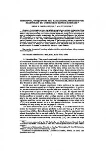
Set X = [1, 2] and Y = [2, 3]. Both are endowed with the Lebesgue measure. Set Z0 = [0, 1] and 1 u (x, z) = − z 2 + xz, u¯ (x) = 0 2 1 2 v (y, z) = yz , v¯ (y) = 0 2 so that suppliers are ordered on the line according to efficiency, the most efficient ones (those with the lowest cost, near y = 2) being on the left, and consumers are ordered according to taste, the most avid ones (those with the highest utility, near x = 2) being on the right (note the order reversal). We compute the lowest ask a (z) and the highest bid b (z): ½ ¾ 1 2 1 b (z) = u¯ (z) = max − z + xz − 0 = − z 2 + 2z 1≤x≤2 2 2 ½ ¾ 1 2 yz − 0 = z 2 a (z) = v¯ (z) = min 2≤y≤3 2 Note that b (z) is the bid price for consumer x = 2 (the most avid one), and a (z) is the ask price for supplier y = 2 (the least efficient one). We have plotted a (z) and b (z) below, where a is the lower curve: 18
p
1.5
1.25
1
0.75
0.5
0.25
0 0
0.25
0.5
0.75
1 z
Highest bid and lowest ask prices Note that the generalized Spence-Mirrlees assumptions (8) and (9) are satisfied: Dx u (x, z) = −z + x Dy v (y, z) = yz and both are injective with respect to z. So Theorem 19 applies, and there is a pure equilibrium, with some degree of uniqueness.We shall now compute it. Assume for the moment that every agent is active. This is possible here since µ (X) happens to be equal to ν (Y ) (in other words, there are as many consumers as suppliers). This means that Za = ∅ = Z b , and Z1 = Z0 , so that we can try the reduction method we described in the preceding section. We start with finding the optimal matching between X and Y . Given x and y, the quality z (x, y) which maximizes the utility of the pair (x, y) is obtained by maximizing the expression −z 2 /2 + xz − yz 2 /2 with respect to z, which yields: x 1+y 1 x2 w (x, y) = 21+y z (x, y) =
where w (x, y) is the resulting utility for the pair. We then seek the measure19
preserving map σ : [1, 2] → [2, 3] which maximizes the integral: Z 2 Z 2 x2 dx w (x, σ (x)) dx = 1 1 1 + σ (x) We have:
x ∂2w =− u¯ (x) for every x and p (y) < −¯ v (y) for every y. This leads us to explicit bounds for c: 2. 196 8 × 10−2 = 5 ln
5 35 5 34 − ≤ c ≤ 5 ln − = 5. 321 8 × 10⁻² 4 32 4 32
(13)
For any c in that the function p (z) given by formula (12) is the £ 1 interval, ¤ 2 restriction to Zt = 4 , 3 of an equilibrium price, the equilibrium supply and demand being given by (11) and (10). We a way that the qualities £ now ¤ have £ 1 to¤ extend pt to Z0 = [0, 1] in such 1 1 z ∈ 0, 3 ∪ 2 , 1 are not traded. For z = 4 , the least efficient supplier y = 3 provides the least avid consumer x = 1, and the price of qualities z ≤ 14 must be such that each of them prefers staying at 14 . This yields the inequalities: µ ¶ µ ¶ 1 1 − v 3, p (z) − v (3, z) ≤ p 4 4 µ ¶ ¶ µ 1 1 − pt u (1, z) − p (z) ≤ u 1, 4 4 and hence:
µ ¶ µ ¶ 1 2 1 1 3 7 3 − z +z− +p ≤ p (z) ≤ p + z2 − 2 32 4 4 2 32
Similarly, for z ≥ 23 , we get the inequalities: µ ¶ µ ¶ 2 2 4 1 2 10 +p ≤ p (z) ≤ p − + z2 − z + 2z − 2 9 3 3 9 In summary, we have: ⎧ − 5 ln 54 ⎨ c − 12 z 2 + z + 34 32 1 2 z + 5z − 5 ln (z + 1) + c p (z) = ⎩ 2 1 2 c − 2 z + 2z − 5 ln 53 + 22 9 ⎧ 5 38 3 2 c − 5 ln 4 + 32 + 2 z ⎨ 1 2 z + 5z − 5 ln (z + 1) + c p (z) = ⎩ 2 c − 5 ln 53 + 28 + z2 9
if 0 ≤ z ≤ 14 if 14 ≤ z ≤ 23 if 23 ≤ z ≤ 1 if 0 ≤ z ≤ 14 if 14 ≤ z ≤ 23 if 23 ≤ z ≤ 1
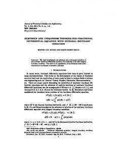
The results are summarized in the next picture, where we have chosen c = 5 ln 54 − 34 (the largest 32 £ 1 value) ¤ and we have incorporated the graphs of 2 a and b. In the £interval , , the 4 £3 ¤ equilibrium price is uniquely defined. ¤ 1 2 In the intervals 0, , 1 , any price schedule which lies between and 4© ª ª 3 © min p , b and max p , a is an equilibrium price. 21
p 1.5 1.25 1 0.75 0.5 0.25 0 0
0.25
0.5
0.75
1 z
Equilibrium Pricing By Theorem 18, s and d are uniquely determined, in the sense that any pure equilibrium such that all agents are active will have the same supply and demand. This implies that the pure equilibria we have just found are ¯ the only ones for which Z0 = Z. We sum up our conclusions. The above picture shows an uppermost and an lowermost curve: these represent the highest bid price and the lowest ask price. Between them, there are £two curves, an upper one and a lower one, ¤ 1 2 which coincide over the interval 4 , 3 . All curves lying between them, and between the two preceding ones, are possible equilibrium prices. 4.4.2
A case when Za is non-empty
Let us now increase the number of consumers: say Y = [2, 3] is unchanged, while X = [h, 2] with 0 < h < 1. Both intervals are endowed with the Lebesgue measure. In equilibrium, if all suppliers are active, then consumers in the range [h, 1] must be priced out of the market. This is done by fixing c in formula (13) to its highest possible value, namely 5 ln 54 − 34 : 32 1 2 5 34 1 for ≤ z ≤ (14) p (z) = z 2 + 5z − 5 ln (z + 1) + 5 ln − 2 4 32 4 3 Then consumer x = 1 makes precisely his/her reservation utility, which means that he/she is indifferent. Recall that d (1) = 14 = s (3). For 0 < z < 14 , consider the bid price for
22
quality z by consumer x = 1: 1 b (1, z) = − z 2 + z 2 £ Consumers of type x < 1 will have a lower bid price. On 0, choose for p a continuous function such that p (1) = pt (1) and µ ¶ µ ¶ 1 4 1 2 1 3 − z + z < p (z) < p − v 3, + v (3, z) = z 2 + 2 4 4 2 32
1 4
¤ , we (15)
The left inequality ensures that consumers or type x < 1 are not bidders for quality z, so they just buy quality 0 at price 0, that is, they revert to their reservation utility. The right inequality ensures that the least efficient producer will not become interested in producing quality z, so that the more efficient ones will not either. £ ¤ For z ∈ ]0, 14 ] we choose a p satisfying (15), in the range 14 , 23 = Zt , the price p is uniquely determined by formula (14),and in the range £equilibrium ¤ 2 , 1 , we can choose p to be any continuous function such that: 3
3 199 1 2 3 295 + − z + 2z ≤ p (z) ≤ 5 ln + + z2 4 144 2 4 144 This is precisely the picture we have drawn in the case h = 1, with a slightly different intepretation. Here the value c = 5 ln 54 − 34 is forced by the 32 fact that the number of consumers is greater than the number of suppliers). We have Zb = {0}, and we note that for all consumers x ∈ [h, 1[ demand is uniquely defined: d (x) = 0. It may be interesting to picture the demand and indirect utility of consumers in equilibrium: 5 ln
23
Demand and indirect utility on X = [h, 1]
5
Open problems.
In this paper, we have assumed that the good is indivisible, and that consumers and producers are limited to buying and selling one unit. That assumption can be relaxed. Indeed, our results carry through if we assume that suppliers, for instance, are restricted to producing one quality, but have the choice of the quantity they produce, their profit then being np − v (y, z, n), where z is the quality produced, n the quantity, p the price, and y the type of the supplier. As we mentioned in the beginning, the main limitation of our model is the assumption that utilities are separable. A truly general model would introduce a quantity good beside the quality good, and consumers of type x would solve the problem: max {u (x, z, t) | p (z) + πt ≤ w} where t is the quantity of the second good, and π its (linear) price. Our methods do not readily apply to this situation, and we plan to investigate it further. Finally, we wish to stress that although we have what appears as a complete equilibrium theory for multidimensional hedonic models, the numerical aspects are far from being as well understood. The method we used in the example is strictly one-dimensional, and there is no easy way to extend it 24
to the multidimensional case. The obvious way to proceed is to follow the theoretical argument, and try to minimize the integral I (p) in (30), but we have made no progress in that direction. It certainly is a good topic for future research. So will all the econometric aspects (characterization and identification). This investigation has been started in [4], but is far from being complete.
References [1] G. Becker (1965) "A study of the allocation of time", Economic Journal 75, p.493-517 [2] G. Carlier (2003) "Duality and existence for a class of mass transportation problems and economic applications", Advances in Mathematical Economics 5, p. 1-21 [3] L. Court (1941) "Entrepreneurial and consumer demand theories for commodity spectra" Econometrica 9, p.135-62 and 241-97 [4] I. Ekeland, J. Heckman and L. Nesheim (2004) "Identification and estimation of hedonic models", Journal of Political Economy 112 (S1), p.60-109 [5] I. Ekeland (2005) "An optimal matching problem", ESAIM: Control, Optimisation and Calculus of Variations, 11 (1) p. 57-71 [6] N. Gretzki, J. Ostroy and W. Zame (1992) "The nonatomic assignment model", Economic Theory 2, p. 103-127 [7] N. Gretzki, J. Ostroy and W. Zame (1999) "Perfect competition in the continuous assignment model", Journal of Economic Theory 88, p. 60118 [8] Z. Griliches ed. (1971) "Price indexes and quality change", Harvard University Press [9] H. Houthakker (1952), "Compensated changes in quantities and qualities consumed", Review of Economic Studies 19 (3), p.155-164 [10] T. Koopmans and M. Beckmann (1957) "Assignment problems and the location of economic activities". Econometrica 25, p. 53-76 [11] K. Lancaster (1966) "A new approach to consumer theory", Journal of Political Economy 74 (2), p.132-157 25
[12] R. Muth (1966) "Household production and consumer demand function". Econometrica 39, p, 699-708 [13] R. Ramachandran and L. Ruschendorf (2004) "Assignment models for constrained marginals and restricted markets", Working paper [14] M. Mussa and S. Rosen (1978) "Monopoly and product quality" , Journal of Economic Theory 18, p.301-317 [15] J.C. Rochet and P. Choné (1998) "Ironing, sweeping and multidimensional screening", Econometrica 66 (4), p.783-826 [16] S. Rosen (1974) "Hedonic prices and implicit markets: product differentiation in pure competition" Journal of Political Economy (82), p. 34-55 [17] L.S. Shapley and M. Shubik (1972) "The assignment game I: the core" International Journal of Game Theory 1‘ (1972), p. 111-130 [18] C. Villani (2003) "Topics in mass transportation", Graduate Studies in Mathematics, AMS.
A
Fundamentals of u-convex analysis.
In this section, we basically follow Carlier [2].
A.1
u-convex functions.
We will be dealing with function taking values in R∪ {+∞}. A function f : X → R∪ {+∞} will be called u-convex iff there exists a non-empty subset A ⊂ Z × R such that: ∀x ∈ X, f (x) = sup {u (x, z) + a}
(16)
(z,α)∈A
A function p : Z → R∪ {+∞} will be called u-convex iff there exists a non-empty subset B ⊂ X × R such that: p (z) = sup {u (x, z) + b} (x,b)∈B
26
(17)
A.2
Subconjugates
Let f : X → R∪ {+∞}, not identically {+∞}, be given. We define its subconjugate f : Z → R∪ {+∞} by: f (z) = sup {u (x, z) − f (x)}
(18)
x
It follows from the definitions that f is a u-convex function on Z (it might be identically {+∞}). Let p : Z → R∪ {+∞}, not identically {+∞}, be given. We define its subconjugate p : X → R∪ {+∞} by: p (x) = sup {u (x, z) − p (z)}
(19)
z
It follows from the definitions that p is a u-convex function on X (it might be identically {+∞}). Example 21 Set f (x) = u (x, z¯) + a. Then f (¯ z ) = sup {u (x, z¯) − u (x, z¯) − a} = −a x
Conjugation reverses ordering: if f1 ≤ f2 , then f1 ≥ f2 , and if p1 ≤ p2 , then p1 ≥ p2 . As a consequence, if f is u-convex, not identically {+∞}, then f is u-convex, not identically {+∞},. Indeed, since f is u-convex, we have f (x) ≥ u (x, z) + a for some (z, a), and then f (z) ≤ −a < ∞. Proposition 22 (the Fenchel inequality) For any functions f : X → R∪ {+∞} and p : X → R∪ {+∞}, not identically {+∞}, we have: ∀ (x, z) , f (x) + f (z) ≥ u (x, z) ∀ (x, z) p (z) + p (x) ≥ u (x, z)
A.3
Subgradients
Let f : X → R∪ {+∞} be given, not identically {+∞}. Take some point x ∈ X. We shall say that a point z ∈ Z is a subgradient of f at x if the points x and z achieve equality in the Fenchel inequality: f (x) + f (z) = u (x, z)
(20)
The set of subgradients of f at x will be called the subdifferential of f at x and denoted by ∂f (x). Specifically: 27
ª © Definition 23 ∂f (x) = arg maxz u (x, z) − f (z)
Similarly, let p : Z → R∪ {+∞} be given, not identically {+∞}. Take some point z ∈ Z. We shall say that a point x ∈ X is a subgradient of p at z if: p (x) + p (z) = u (x, z) (21) The set of subgradients of p at z will be called the subdifferential of p at z and denoted by ∂p (z). ª © Definition 24 ∂p (z) = arg maxx u (x, z) − p (x)
Proposition 25 The following are equivalent: 1. z ∈ ∂f (x) 2. ∀x0 , f (x0 ) ≥ f (x) + u (x0 , z) − u (x, z)
If equality holds for some x0 , then z ∈ ∂f (x0 ) as well. Proof. We begin with proving that the first condition implies the second one. Assume z ∈ ∂f (x). Then, by (20) and the Fenchel inequality, we have: f (x0 ) ≥ u (x0 , z) − f (z) = u (x0 , z) − [u (x, z) − f (x)] We then prove that the second condition implies the first one. Using the inequality, we have: f (z) = sup {u (x0 , z) − f (x0 )} x0
≤ sup {u (x0 , z) − f (x) − u (x0 , z) + u (x, z)} x0
= u (x, z) − f (x) so f (x) + f (z) ≤ u (x, z). We have the converse by the Fenchel inequality, so equality holds. Finally, if equality holds for some x0 in condition (2), then f (x0 ) − u (x0 , z) = f (x) − u (x, z), so that: ∀x00 , f (x00 ) ≥ f (x) − u (x, z) + u (x00 , z) = f (x0 ) − u (x0 , z) + u (x00 , z) which implies that z ∈ ∂f (x0 ). There is a similar result for functions p : Z → R∪ {+∞}, not identically {+∞}: we have x ∈ ∂p (z) if and only if ¡ ¢ ¡ ¢ ¡ ¢ (22) ∀ x0 , Z¯ , p Z¯ ≥ p (z) + u x, Z¯ − u (x, z) 28
A.4
Biconjugates
It follows from the Fenchel inequality that, if p : Z → R∪ {+∞} is not identically {+∞}: ª © p (z) = sup u (x, z) − p (x) ≤ p (z)
(23)
x
Example 26 Set p (z) = u (¯ x, z) + b. Then ª © p (z) = sup u (x, z) − p (x) x
≥ u (¯ x, z) − p (¯ x) = u (¯ x, z) + b = p (z)
This example generalizes to all u-convex functions. Denote by Cu (Z) the set of all u-convex functions on Z. Proposition 27 For every function p : Z → R∪ {+∞}, not identically {+∞}, we have p (z) = sup {ϕ (z) | ϕ ≤ p, ϕ ∈ Cu (Z)} ϕ
Proof. Denote by p¯ (z) the right-hand side of the above formula. We want to show that p (z) = p¯ (z) Since p ≤ p and p is u-convex, we must have p ≤ p¯. On the other hand, p¯ is u-convex because it is a supremum of u-convex functions. So there must be some B ⊂ X × R such that: p (z) = sup {u (x, z) + b} (x,b)∈B
Let (x, b) ∈ B. Since p¯ ≤ p, we have u (x, z) + b ≤ p¯ (z) ≤ p (z). Taking biconjugates, as in the preceding example, we get u (x, z) + b ≤ p (z). Taking the supremums over (x, b) ∈ B, we get the desired result. Corollary 28 Let p : Z → R∪ {+∞} be a u-convex function, not identically {+∞}. Then p = p , and the following are equivalent: 1. x ∈ ∂p (z) 2. p (z) + p (x) = u (x, z) 3. z ∈ ∂p (x) 29
Proof. We have p ≤ p always by relation (23). Since p is u-convex, we have: p (z) = sup {u (x, z) + b} (x,b)∈B
for some B ⊂ X × R. By proposition 27, we have: sup {u (x, z) + b} ≤ p (z)
(x,b)∈B
and so we must have p = p . Taking this relation into account, as well as the definition of the subgradient, we see that condition (2) is equivalent both to (1) and to (2) Definition 29 We shall say that a function p : Z → R∪ {+∞} is u-adapted if it is not identically {+∞} and there is some (x, b) ∈ X × R such that: ∀z ∈ Z, p (z) ≥ u (x, z) + b It follows from the above that if p is u-adapted, then so are p , p and all further subconjugates. Note that a u-convex function which is not identically {+∞} is u-adapted. Corollary 30 Let p : Z → R∪ {+∞} be u-adapted. Then : p
=p
Proof. If p is u-adapted, then p is u-convex and not identically {+∞}. The result then follows from corollary 28.
A.5
Smoothness
Since u is continuous and X × Z is compact, the family {u (x, ·) | x ∈ X } is uniformly equicontinuous on Z. It follows from definition 16 that all uconvex functions on Z are continuous (in particular, they are finite everywhere).. Denote by k the upper bound of kDx u (x, z)k for (x, z) ∈ X × Z. Since Dx u is continuous and X × Z is compact, we have k < ∞, and the functions x → u (x, z) are all k-Lipschitzian on X. Again, it follows from the definition 16 that all u-convex functions on X are k-Lipschitz (in particular, they are finite everywhere). By Rademacher’ theorem, they are differentiable almost everywhere with respect to the Lebesgue measure. 30
Let f : X → R be convex. Since f = f , we have: ª © f (x) = sup u (x, z) − f (z) z
Since f is u-convex, it is continuous, and the supremum is achieved on the right-hand side, at some point z ∈ ∂f (x). This means that all u-convex functions on X are subdifferentiable everywhere on X. The following result will also be useful: Proposition 31 Let p : Z → R be u-adapted, and let x ∈ X be given. Then there is some point z ∈ ∂p (x) such that p (z) = p (z). Proof. Assume otherwise, so that for every z ∈ ∂p (x) we have p (z) < p (z). For every z ∈ ∂p (x), we have x ∈ ∂p (z), so that, by proposition 25, we have p (z 0 ) ≥ u (x, z 0 ) − u (x, z) + p (z)
for all z 0 ∈ Z, the inequality being strict if z 0 ∈ / ∂p (x) . Set ϕz (z 0 ) = u (x, z 0 ) − u (x, z) + p (z). We have: / ∂p (x) =⇒ ϕz (z 0 ) < p (z 0 ) ≤ p (z 0 ) z0 ∈ z 0 ∈ ∂p (x) =⇒ ϕz (z 0 ) ≤ p (z 0 ) < p (z 0 )
so that ϕz (z 0 ) < p (z 0 ) for all (z, z 0 ). Since Z is compact, there is some ε > 0 such that ϕz (z 0 ) + ε ≤ p (z 0 ) for all (z, z 0 ). Taking the subconjugate with respect to z 0 , we get: p (x) ≤ sup {u (x, z 0 ) − ϕz (z 0 )} − ε z0 © ª = sup u (x, z 0 ) − u (x, z 0 ) + u (x, z) − p (z) − ε z0
= u (x, z) − p (z) − ε = p (x) − ε
which is a contradiction. The result follows Corollary 32 If ∂p (x) = {z} is a singleton, then: p (z) = p (z)
(24)
p (x) = u (x, z) − p (z)
(25)
and: Proof. Just apply the preceding proposition, bearing in mind that ∂p (x) contains only one point, namely ∇u p (x). This yields equation (24) Equation (25) follows from the definition of the subgradient and equation (24). 31
A.6
v-concave functions.
˙ Given v : Y × Z → R, we Let us now consider the duality between Y and Z. say that a map g : Y → R∪ {−∞} is v-concave iff there exists a non-empty subset A ⊂ Z × R such that: ∀y ∈ Y, g (y) = inf {v (y, z) + a} (z,α)∈A
(26)
and a function p : Z → R∪ {−∞} will be called v-concave iff there exists a non-empty subset B ⊂ X × R such that: p (z) = inf {v (y, z) + b} (x,b)∈B
(27)
All the results on u-convex functions carry over to v-concave functions, with obvious modifications. The superconjugate of a function g : Y → R∪ {−∞}, not identically {−∞}, is defined by: g (z) = inf {v (y, z) − g (y)} y
(28)
and the superconjugate of a function p : Z → R∪ {−∞}, not identically {−∞}, is given by: p (y) = inf {v (y, z) − p (z)} (29) z
The superdifferential ∂p is defined by: ∂p (y) = arg min {v (y, z) − p (z)} z
and we have the Fenchel inequality: p (z) + p (y) ≤ v (y, z) ∀ (y, z) with equality iff z ∈ ∂p (y). Note finally that p ≥ p, with equality if p is v-concave
B
Some notations and definitions.
B.1
Radon measures and probabilities.
With a locally compact set Ω (such as an open subset of the compact set Z) we will associate the following sets of functions and measures on Ω: • K (Ω), the space of continous functions on Ω with compact support 32
• C b (Ω) , the space of bounded continous functions on Ω • C+ (Ω), the cone of non-negative functions • M (Ω), the space of measures on Ω • M+ (Ω) ⊂ M (Ω), the cone of positive measures • Mb (Ω) ⊂ M (Ω), the cone of finite measures • Mb+ (Ω) = Mb (Ω) ∩ M+ (Ω), the cone of positive finite measures • P (Ω) ⊂ Mb+ (Ω) the set of probabilities on Ω The space K (Ω) will be endowed with the topology of uniform convergence on compact subsets of Ω, and the space C b (Ω) with the uniform norm. Then C b (Ω) is a Banach space, but K (Ω) is not, unless Ω is compact, in which case all continuous functions on Ω are bounded, and we have C (Ω) = K (Ω) = C b (Ω). When Ω is finite and has d elements, all these spaces coincide with Rd . We take measures in the sense of Radon, that is, M (Ω) is defined to be the dual of K (Ω) and Mb (Ω) is defined to be the dual of C b (Ω). So Mb (Ω) is a Banach space, but M (Ω) is not, unless Ω is compact, in which case M (Ω) = Mb (Ω), that is, all Radon measures on Ω Rare finite. For γ ∈ M (Ω) and ϕ ∈ K (Ω),we write indifferently < γ, ϕ > or Z ϕdγ. A probability γ ∈ P (Z) is defined as a non-negative bounded measure such that < γ, 1 >= 1. The set P (Z) is convex, and is compact in the weak* topology: γn → γ if < γn , ϕ >→< γ, ϕ > for every ϕ ∈ C b (Ω). We say that a measure γ is carried by K if < γ, ϕ >= 0 for all ϕ ∈ K (Ω) which vanish on K. If γ is carried by a subset K, it is also carried by its closure. The support of a measure γ, denoted by Supp (γ), is the smallest closed set K such that γ is carried by K.
B.2
Conditional probabilities and marginals.
Given a positive measure αX×Z ∈ M+ (X × Z) (which has to be finite, since X ×Z is compact) we define its marginals αX ∈ M+ (X) and αZ ∈ M+ (Z)as follows: Z
ϕ (x) dαX =
X
Z
Z
Z
ϕ (x) dαX×Z
∀ϕ ∈ K (X)
ψ (z) dαX×Z
∀ψ ∈ K (Z)
X×Z
ψ (z) dαZ =
Z
X×Z
33
and we denote the probability of the second coordinate being z conditional on the first coordinate being x by Pxα (z). The mathematical expectation with respect to this probability will be denoted by Exα : Z α ψ (z) dPxα (z) Ex [ψ] = Z
This conditional probability is related to the first marginal by the formula: Z Z f (x, z) dαX×Y = Exα [f (x, z)] dαX ∀f ∈ K (X × Z) X×Z
X
Similar considerations hold for positive measures βY ×Z ∈ M+ (Y × Z), We have: Z Z ϕ (y) dβY = ϕ (y) dβY ×Z ∀ϕ ∈ K (Y ) Y Y ×Z Z Z ψ (z) dβZ = ψ (z) dβY ×Z ∀ψ ∈ K (Z) Z X×Z Z Z g (y, z) dβY ×Z = Eyβ [g (y, z)] dβY ∀g ∈ K (Y × Z) Y ×Z
C
Y
Proof of the Existence Theorem
C.1
The dual problem: existence
Recall that Z = {∅d } ∪ Z0 ∪ {∅s } ,with Z1 = {z | a (z) ≤ b (z)} a compact non-empty subset of Z0 . Denote by A the set of all admissible price systems on Z, that is, the set of all continuous maps p : Z → R which satisfy: ∀z ∈ Z1 ,
a (z) ≤ p (z) ≤ b (z)
A is a non-empty, convex and closed subset of K (Z) , the space of all continuous function on Z. Now define a map I : K (Z) → R by: Z Z I (p) = p (x) dµ − p (y) dν (30) X
Y
Proposition 33 The map I is convex
Proof. Take p1 and p2 in A. Take s and t in [0, 1] with s + t = 1. Then: (sp1 + tp2 ) (x) = sup {u (x, z) − sp1 (z) − tp2 (z)} z
= sup {s [u (x, z) − p1 (z)] + t [u (x, z) − p2 (z)]} z
≤ s sup {u (x, z) − p1 (z)} + t sup {u (x, z) − p2 (z)} z
z
= sp1 (x) + tp2 (x) 34
Similarly, we find that: (sp1 + tp2 ) (y) ≥ sp1 (x) + tp2 (x) Integrating, we find that I is convex, as announced. Now consider the convex optimization problem: (31)
inf I (p)
p∈A
Proposition 34 The set of solutions of problem (P) is convex. This follows from the fact that we are minimizing a convex function on a convex set. We have to show that this set is non-empty. The following lemma will be useful. Lemma 35 Assume p is admissible. Set: © ª pa (z) = max p (z) , a (z)
¡ ¢ Then pa = p
¡ ¢ Proof. We have p ≤ pa ≤ p. Taking conjugates, we get p ≤ pa ≤ ¡ ¢ =p. p ¡ ¢ © ª Similarly, we find that pb = p , with pb = min p , b
Proposition 36 Problem (P) has a solution.
Proof. Take a minimizing sequence pn . Since the functions pn (resp. pn ), n ∈ N, are u-convex (resp. v-concave), they are uniformly Lipschitzian (see section A), and hence equicontinuous. By Ascoli’s theorem we can extract uniformly convergent subsequences (still denoted by pn and pn ) : pn → f pn → g
so that: Z
X
f (x) dµ −
Z
Y
g (y) dν = inf
a≤p≤b
∙Z
X
p (x) dµ −
Z
Y
p (y) dν
¸
(32)
It is easy to see that f is u-convex and g is v-concave. In addition, pn → f and pn → g everywhere (and uniformly as well, since the functions 35
are equicontinuous). Since pn ≤ pn , we get f ≤ g in the limit. Since pn ≤ b, we have pn ≤ b = b, and letting n → ∞, we find that f ≤ b. Since f is u-convex, it is continuous (and even Lipschitzian, see section A). Similarly, g is v-concave, hence continuous, and satisfies g ≥ a. Now take any continuous price schedule p¯ such that © ª © ª ¡ ¢ ¡ ¢ (33) f a = max f , a ≤ p¯ ≤ min g , b = g b ª © ª¢ ¡ © for instance p¯ = 12 max f , a + min g , b . By Lemma 35, we have ³¡ ¢ ´ f a =f =f ³¡ ¢ ´ g b =g =g
the last equalities occuring because f is u-convex and g is v-concave. Taking conjugates in formula (33), we get g ≤ p¯ and f ≥ p¯ .Substituting in the integral, we get: Z Z Z Z p¯ (x) dµ − p¯ (y) dν ≤ f (x) dµ − g (y) dν X
Y
X
Y
and hence, by formula (32): ∙Z ¸ Z Z Z p¯ (x) dµ − p¯ (y) dν ≤ inf p (x) dµ − p (y) dν X
Y
a≤p≤b
X
Y
Since p¯ is admissible, p¯ must be a minimizer, and the result follows. The proof indicates that uniqueness is not to be expected. The following result is the Non-Uniqueness Theorem for prices: Proposition 37 Let p be a solution of problem (P). Then pa and pb are also solutions. More generally, if q is an admissible price schedule such that: pa (z) ≤ q (z) ≤ pb (z)
∀z ∈ Z1
then q is a solution of problem (P). ¡ ¢ Proof. From pa ≤ q ≤ pb , we deduce that p = pb ≤ q and that ¡ ¢ q ≤ pa = p . Substituting into the integral, we get: Z Z Z Z q (x) dµ − q (y) dν ≤ p (x) dµ − p (y) dν = inf (P ) X
Y
X
and since q is admissible, it must be a minimizer. 36
Y
¡ ¢ Corollary 38 Let p be a solution of problem (P). Then p = pb , µ-almost ¡ ¢ everywhere, and p = pa , ν-almost everywhere.
Proof. ¡ ¢ By the preceding Proposition, pb is a solution of problem (P), so that I pb = I (p) .Substituting in the integrals, we get: Z Z Z Z ¡ ¢ ¡ ¢ p (x) dµ − p (y) dν pb dµ − pb dν = X
Y
X
Y
¡ ¢ and since pb = p , this reduces to: Z Z ¡ ¢ p (x) dµ pb dµ = X
X
¡ ¢ Since pb ≤ p, we have pb ≥ p , and since the integrals are equal, it ¡ ¢ ¡ ¢ follows that p = pb , µ-a.e. The same argument shows that p = pa , ν-a.e. Corollary 39 Let p be a solution of problem (P). Then, for µ-almost every x in X, there is a point z ∈ D (x) such that p (z) = pb (z) , and for ν-almost every y in Y , there is a point z ∈ S (y) such that p (z) = pa (z) ¡ ¢ Proof. Fix an x such that p (x) = pb (x) and consider the functions ϕ and ψ defined by ϕ (z) = u (x, z) − p (z) and ψ (z) = u (x, z) − pb (z). We have ϕ ≥ ψ, and max ϕ = max ψ. So there must be a point z¯ such that max ϕ = max ψ = ϕ (¯ z ) = ψ (¯ z ) .The result follows. Note that we already have p (z) = p (z) for every z ∈ D (x), and p (z) = p (z) for every z ∈ S (y)
C.2
The dual problem: optimality conditions
Recall that we have defined a map I : K (Z) → R by: Z Z p (x) dµ − p (y) dν I (p) = X
Y
We have checked that the function I is convex. It is easily seen to be continuous: if pn → p uniformly on Z, then pn → p uniformly on X and pn → p uniformly on Y . On the other hand, the set A is non-empty, convex and closed in K (Z). This means that the constraint qualification conditions hold in problem (P): a necessary and sufficient condition for p¯ to be optimal is that: 0 ∈ ∂I (¯ p) + NA (¯ p) (34) 37
where ∂I (¯ p) is the subgradient of I at p¯ in the sense of convex analysis, and NA (¯ p) is the normal cone to A at p¯. All we have to do now is to compute both of them. C.2.1
Computing ∂I (p)
Lemma 40 Let p ∈ K (Z) and ϕ ∈ K (Z). Then, for every x ∈ X and every y ∈ Y , we have: i 1h lim (p + hϕ) (x) − p (x) = − min {ϕ (z) | z ∈ D (x)} h→0 h h>0 i 1h lim (p + hϕ) (y) − p (y) = − max {ϕ (z) | z ∈ S (y)} h→0 h h>0
Proof. Let us prove the second equality; the first one is derived in a similar way. Take z ∈ Sp (y) and zh ∈ Sp+hϕ (y). From the definition of Sp (y) and Sp+hϕ (y), we have: v (y, zh ) − p (zh ) ≥ p (y) = v (y, z) − p (z)
v (y, z) − p (z) − hϕ (z) ≥ (p + hϕ) (y) = v (y, zh ) − p (zh ) − hϕ (zh ) Substracting, we find that: −hϕ (z) ≥ (p + hϕ) (y) − p (y) ≥ −hϕ (zh )
(35)
Since z is an arbitrary point in Sp (y), we can take it to be the minimizer on the left-hand side, and this inequality becomes: −h max {ϕ (z) | z ∈ Sp (y)} ≥ (p + hϕ) (y) − p (y) ≥ −hϕ (zh ) Now let h → 0. The family zh ∈ Sp+hϕ (y) must have cluster points, because Z is compact, and any cluster point z¯ must belong to Sp (y). Taking limits in inequality (35), we find that, for some z¯ ∈ Sp (y): i 1h − max {ϕ (z) | z ∈ Sp (y)} ≥ lim (p + hϕ) (y) − p (y) ≥ −ϕ (¯ z ) (36) h→0 h h>0
and the result follows. Because of inequality (36), we can apply the Lebesgue convergence theorem, and we get: Z Z 1 lim [I (p + hϕ) − I (p)] = max {ϕ (z) | z ∈ S (y)} dν− min {ϕ (z) | z ∈ D (x)} dµ h→0 h Y X h>0 (37) 38
We now work on the right-hand side of formula (37). Define B (X, D) to be the set of all Borel maps d : X → Z such that d (x) ∈ D (x) for every x. Similarly, B (Y, S) is the set of all Borel maps s : Y → Z such that s (y) ∈ S (y) for every y. Lemma 41 For every ϕ ∈ C (Z), we have: ½Z ¾ Z min {ϕ (z) | z ∈ D (x)} dµ = min ϕ (d (x)) dµ | d ∈ B (X, D) X
Z
Y
X
max {ϕ (z) | z ∈ S (y)} dν = max
½Z
X
(38) ¾ ϕ (s (y)) dµ | s ∈ B (Y, S)
(39)
Proof. Given ϕ ∈ C (Z), the multivalued maps Γ1 and Γ2 defined by: Γ1 (x) = arg min {ϕ (z) | z ∈ D (x)} Γ2 (y) = arg max {ϕ (z) | z ∈ S (y)} have compact graph. Formulas (38) and (39) then follow from a standard measurable selection theorem. Define M+ (X, D) to be the set of all demand distributions, that is, the set of all positive measures αX×Z on X × Z which are carried by the graph of D and which have µ as marginal: αX = µ Recall that αZ ∈ M+ (Z) denotes the second marginal of αX×Z . Lemma 42 For every ϕ ∈ K (Z), we have: ½Z ¾ Z min {ϕ (z) | z ∈ D (x)} dµ = min ϕdαZ | αX×Z ∈ M+ (X, D) X
Z
(40)
Proof. Let us investigate the right-hand side of formula (38). Let f ∈ B (X, D) be such that ϕ (f (x)) = min {ϕ (z) | z ∈ D (z)} for µ-almost every x, and define γX×Z ∈ M+ (X, D) by: Z Z ∀ψ ∈ K (X × Z) , ψ (x, z) dγX×Z = ψ (x, f (x)) dµ X×Z
X
39
Clearly: ½Z ¾ Z min ϕ (d (x)) dµ | d ∈ B (X, D) = ϕ (f (x)) dµ X Z ZX ϕdγX×Z = ϕdγZ = X×Z Z ½Z ¾ ≥ min ϕdαZ | αX×Z ∈ M+ (X, D) Z
For the reverse inequality, we take any αX×Z ∈ M+ (X, D). Taking conditional expectations, we have: Exα [ϕ] ≥ min {ϕ (z) | z ∈ D (x)} and by integrating with respect to µ, we get the desired result: Z Z ϕdαZ ≥ min {ϕ (z) | z ∈ D (x)} dµ Z X ¾ ½Z ϕ (z) dµ | z ∈ D (x) = min X ¾ ½Z ϕ (d (x)) dµ | d ∈ B (X, D) = min X
Considering the set M+ (Y, S) of supply distributions, we get similar results: ½Z ¾ Z max {ϕ (z) | z ∈ S (y)} dν = max ϕdβZ | βY ×Z ∈ M+ (Y, S) (41) Y
Z
Writing formulas (40) and (41) in formula (37), we get: 1 [I (p + hϕ) − I (p)] h→0 h h>0 ½Z ¾ ½Z ¾ = max ϕdβZ | βY ×Z ∈ M+ (Y, S) − min ϕdαZ | αX×Z ∈ M+ (X, D) Z Z ¾ ½Z Z ϕdβZ − ϕdαZ | βY ×Z ∈ M+ (Y, S), αX×Z ∈ M+ (X, D) = max lim
Z
Z
Proposition 43 The subdifferential of I at p is given by: ∂I (p) = {βZ − αZ | βY ×Z ∈ M+ (Y, S), αX×Z ∈ M+ (X, D)} 40
Proof. Take λ ∈ M (Z) = Mb (Z). By definition of the subgradient, λ ∈ ∂I (p) if and only if, for every ϕ ∈ K (Z) and h > 0, we have: Z I (p + hϕ) ≥ I (p) + h ϕdλ Z
Since I is convex, this is equivalent to: Z 1 ϕdλ lim [I (p + hϕ) − I (p)] ≥ h→0 h Z h>0
Because of formula (37), this is equivalent to: ½Z ¾ Z Z max ϕdβZ − ϕdαZ | βY ×Z ∈ M+ (Y, S), αX×Z ∈ M+ (X, D) ≥ ϕdλ Z
Z
This means that λ belongs to the closed convex set:
{βZ − αZ | βY ×Z ∈ M+ (Y, S), αX×Z ∈ M+ (X, D)} C.2.2
Computing NA (p)
Take λ ∈ M (Z) = Mb (Z). By definition, λ ∈ NA (p) if and only if, for every q ∈ A , we have: Z Z
(q − p) dλ ≤ 0
Since q (∅d ) = p (∅d ) = 0 and q (∅s ) = p (∅s ) = 0 for every q ∈ A, this condition is equivalent to: Z (q − p) dλ ≤ 0 (42) Z0
To interpret this condition, we need some notation. Set: Z b = {z ∈ Z0 | a (z) < p (z) = b (z)}
Zab Za M N
= {z = {z = {z = {z
∈ Z0 ∈ Z0 ∈ Z0 ∈ Z0
| | | |
a (z) < p (z) < b (z)} a (z) = p (z) < b (z)} a (z) = p (z) = b (z)} a (z) > b (z)}
so that we have a partition of Z0 into subsets Z0 = Za ∪ Zab ∪ Z b ∪ M ∪ N, where Za ∪ Zab ∪ Z b ∪ M = Z1 , the set of marketable qualities. Denote by λb , λba , λa , λM , λN the restrictions of λ to Z b , Zab , Za , ZM , ZN respectively. Note that since λ was a bounded measure, so are λb , λba , λa , λM and λN . Condition (42) is equivalent to the following: λb ≥ 0, λba = 0, λa ≤ 0, λN = 0 41
(43)
C.2.3
Concluding the proof.
Let p¯ be a solution of problem (P). By condition (34), we have 0 ∈ ∂I (¯ p) + NA (¯ p). By Proposition 43 , this means that there exists βY ×Z ∈ M+ (Y, S), αX×Z ∈ M+ (X, D) and λ ∈ M (Z) satisfying (43) such that αZ − βZ = λ. In other words, the restriction of αZ − βZ to Z b , Zab , Za respectively are positive, zero and negative: αZ ≥ βZ on Z b
αZ = βZ on Zab αZ ≤ βZ on Za αZ = βZ on N
There is no condition on the restriction of αZ or βZ to {∅d }, {∅s } or M. Since Pxα is carried by D (x), we must have Pxα (z) = 0 whenever z ∈ / D (x), which certainly is the case when p (z) > b (z). Similarly, Pyβ (z) = 0 when p (z) < a (z). If z ∈ N, either p (z) > b (z) or p (z) < a (z), so either Pxα (z) = 0 or Pyβ (z) = 0. The condition αZ = βZ on N then implies that: αZ = βZ = 0 on N 0 We will now show that there exists αX×Z ∈ M+ (X, D) and βY0 ×Z ∈ M+ (Y, S) such that αZ0 = βZ0 . This will be done by suitably modifying αX×Z and βY ×Z . The procedure is best explained in the case when X, Y and Z are discrete sets. We will not give the details of the continuous case, which is a technical implementation of the same idea. Let z¯ ∈ Z0 and assume αZ (¯ z ) 6= βZ (¯ z ). Then either αZ (¯ z ) > βZ (¯ z ) or βZ (¯ z ) > αZ (¯ z ). If αZ (¯ z ) > βZ (¯ z ), then z¯ ∈ Z b , so that a (¯ z ) < p (¯ z ) = b (¯ z ). This implies that all the consumers which have z¯ in their demand set are actually indifferent between buying z¯ and staying out of the market. Denote by ∆ (¯ z) α the set of x such that Px (¯ z ) > 0. We have:
x ∈ ∆ (¯ z ) =⇒ ∅d ∈ D (x) X αZ (¯ z) = Pxα (¯ z ) µ [x] x∈∆(z)
We then pick some x ∈ ∆ (¯ z ) and shift their demand from z¯ to ∅d until the balance between aggregate demand and aggregate supply for z¯ is restored. This can be done in many different ways. For instance, set: 0
Pxα (¯ z) =
βZ [z] α P (¯ z) αZ [z] x 42
∀x ∈ ∆ (z)
We then have: X z] X α βZ [¯ 0 z] = Pxα (¯ z ) µ (x) = Px (¯ z ) µ (x) = β [¯ z] αZ0 [¯ αZ [¯ z] x∈∆(z)
x∈∆(z)
If α (¯ z ) < β (¯ z ), then z¯ ∈ Za , so that a (¯ z ) = p (¯ z ) < b (¯ z ). This implies that all the producers who have z¯ in their demand set are actually indifferent between supplying z¯ and staying out of the market: z ) > 0 =⇒ ∅s ∈ S (y) Pyβ (¯ We then shift some of the supply to ∅s , as we did for the demand. We 0 end up with αX×Z ∈ M+ (X, D) and βY0 ×Z ∈ M+ (Y, S) which satisfy the conclusions of the Existence Theorem.
D
Remaining proofs
D.1
Pareto optimality of equilibrium allocations
0 With every pair of demand and supply distributions, αX×Z ∈ M+ (X, D) 0 and βY ×Z ∈ M+ (Y, S), we associate the number:
¡ 0 ¢ J αX×Z , βY0 ×Z =
=
Z
0 u (x, z) dαX×Z
X×Z
Z
X
0 Exα
−
Z
Y ×Z
[u (x, z)] dµ (x) −
Z
v (y, z) dβY0 ×Z 0
Eyβ [v (y, z)] dν (y)
Y
Assume that αZ0 0 = βZ0 0 .We claim that: Z Z 0 α0 Ex [p (z)] dµ (x) − Eyβ [p (z)] dν (y) = 0 X
µZ
(44)
Y
Indeed, the left-hand side can be written as: ¶ Z 0 0 p (z) dαZ − p (z) dβZ +p (∅d ) (αZ0 [∅d ] − βZ0 [∅d ])+p (∅s ) (αZ0 [∅s ] − βZ0 [∅s ])
Z0
Z0
The first term vanishes because αZ0 0 = βZ0 0 , and the two next terms vanish because p (∅d ) = p (∅s ) = 0. Substracting (44) from J, we get: Z Z ¡ 0 ¢ 0 0 α0 Ex [u (x, z) − p (z)] dµ (x)− Eyβ [v (y, z) − p (z)] dν (y) J αX×Z , βY ×Z = X
Y
43
(45)
By Fenchel’s inequality, (u (x, z) − p (z)) ≤ p (x) for all z ∈ Z. Taking 0 expectations with respect to the probability Pxα , we get: 0
Exα [u (x, z) − p (z)] ≤ p (x)
(46)
with equality if and only if u (x, z)−p (z) = p (x) (in other words, z ∈ D (x)) 0 for Pxα -almost every z ∈ Z. Similarly, we have: 0
Eyβ [v (y, z) − p (z)] ≥ p (y)
(47)
with equality if and only if v (y, z) − p (z) = p (y) (in other words, z ∈ S (y)) 0 for Pyβ -almost every z ∈ Z. Writing this in (45), and treating the second term in the same way, we get: Z Z ¡ 0 ¢ 0 J αX×Z , βY ×Z ≤ p (x) dµ − p (y) dν (48) X
Y
The right-hand side is equal to J (αX×Z , βY ×Z ), for any equilibrium allocation (α, β). This proves that equilibrium allocations solve the planner’s problem, and as such they are Pareto optimal.
D.2
Uniqueness of equilibrium allocations
Observe that equality holds in (48) if and only if equality holds in (46) for µ-almost every x, and equality holds in (47) for ν-almost every y. This means 0 0 that Pxα [D (x)] = 1 for µ-almost every x and Pyβ [S (y)] = 1 for ν-almost every y.
D.3
Proof of Theorem 19
Let (p, αX×Z , βY ×Z ) be an equilibrium. By Rademacher’s theorem, since p : X → R is Lipschitz, and µ is absolutely continuous with respect to the µ-almost everywhere. Lebesgue measure, p is differentiable © ª Consider the set A = x | p (x) ≥ 0 . Let x ∈ A be a point where p is differentiable, with derivative Dx p (x). Since x is active or indifferent, the set D (x) ∩ Z0 is non-empty, and we may take some z ∈ D (x) ∩ Z0 . Consider the function ϕ (x0 ) = u (x0 , z) − p (z). By proposition 25, since D (x) ⊂ ∂p (x), we have ϕ ≤ f and ϕ (x) = f (x), so that ϕ and f must have the same derivative at x : Dx f (x) = Dx u (x, z) (49) By condition (8), this equation defines z uniquely. In other words, for µ-almost every point x ∈ A, the set D (x)©∩ Z0 consists ªof one point only. Similarly, for ν-almost every point y ∈ B = y | p (y) ≤ 0 , the set S (y)∩Z0 consists of one point only. This is the desired result. 44