Subdivision of the Regional Railways North East Network. In 1996 RRNE commissioned our Group to produce schedules for their whole. Monday to Friday ...
University of Leeds
SCHOOL OF COMPUTER STUDIES RESEARCH REPORT SERIES Report 2000.09
Experiences with a Flexible Driver Scheduler| by
Sarah Fores, Les Proll & Anthony Wren April 2000
|
To be presented at CASPT2000, Berlin, June 2000
Abstract. We present a exible user-driven ILP tool for the optimisation compo-
nent of the TRACS II driver scheduling system. The system allows the user to select from a number of objective functions and to drive the LP relaxation through one of a range of optimisation processes. As a default we provide a Sherali objective which minimises the number of shifts, and within that yields the least cost. The default method of solving the LP relaxation is by specialised primal column generation for larger problems, and by dual steepest edge for smaller ones. The LP is capable of working with over 200,000 previously generated shifts. Once the relaxed LP has been solved, we reduce the size of the problem, and enter a specialised branch and bound procedure. Using real data we show how, by being able to handle larger problems, our system reduces the need for problem decomposition and can produce better schedules.
1 Introduction Transport operators typically require an allocation of vehicles to predetermined journeys, an allocation of drivers to vehicles, and rostering of people to a sequence of shifts. Previous workshops (see, e.g.,Desrochers and Rousseau (1992); Daduna et al. (1995); Wilson (1999)) have included attempts to combine vehicle and driver scheduling (see Freling et al. (1999)), but tend to favour approaches which schedule vehicles in advance (see e.g.,Caprara et al. (1999); Rousseau (1995)). TRACS II, developed at the University of Leeds, is a mathematical programming based bus and train driver scheduling system. The system is based upon the IMPACS system (see Smith and Wren (1988); Wren and Smith (1988)) which rst generates valid shifts, and then selects a subset which covers all of the vehicle work and minimises an objective function. The main enhancements made to the Integer Linear Programming (ILP) component relate to the implementation of a choice of solution methods, and to improvements in the size of problem that can be dealt with. Thus, whilst TRACS II has been shown to successfully solve real scheduling problems, the ability to solve ever larger problems enables the user to generate more and better shifts from which a selection can be made, and reduces the need to decompose the problem into smaller areas. This, in turn, is expected to yield better solutions.
2 Driver Scheduling The main information received from the vehicle schedule is the time and location of convenient changeover points for drivers. These location/time pairs are known as relief opportunities and include those at the beginning and end of the vehicle work where a driver will travel with the vehicle to and from the appropriate depot. The periods of time between the relief opportunities are known as pieces of work. Before the driver scheduling can take place it may also be necessary to note that certain vehicles or routes may only be driven 1
by a subset of drivers. Driver scheduling consists of allocating all pieces of work to a set of drivers in such a way that the work of a driver (a shift) is acceptable to union regulations and the schedule is in some way e�cient. The cost of the nal schedule may be determined by the number of shifts included, the actual wage costs according to the hours worked, a penalty cost to deter features which are 'legal' but undesirable, or any combination of all three. The driver scheduling problem has been tackled by many di�erent approaches. Most commercial software, including TRACS II, uses a mathematical programming approach which utilises a set covering or set partitioning formulation to ensure that vehicle work is covered, with a suitable objective function to di�erentiate between schedules. The problem with many such formulations is the large number of variables necessary to produce good schedules, which may lead to the formulation being intractable in a viable computing time. Genetic algorithms (see Kwan et al. (1999)) and constraint satisfaction (see Curtis et al. (1999)) have been investigated as techniques which attempt to nd good schedules using variants of local search. They have the advantage that they can always nd a schedule where sometimes an 'optimisation' approach might not nd a solution within the computing limits or with an imposed target number of shifts. However these techniques currently are at an experimental stage and cannot, in general, match the performance of our ILP approach. Nor currently can they handle side constraints. Algorithmic and technological improvements continue to alleviate the inherent di�culties that mathematical programming techniques have with large problems.
3 TRACS II There are three stages to the solution process of TRACS II : � Generate a set of valid shifts � Reduce the shift set (if required) � Select a subset of shifts which cover the vehicle work and minimises an objective function Each of these sections allows the user exibility in terms of what they want to achieve, making experimentation a viable option.
3.1 Shift Generation Parameter-driven heuristics are employed to rst generate a set of shifts which are valid according to a set of labour agreement rules. The capabilities of these heuristics have been adapted and improved over the years so that many different user requirements can be satis ed within a uni ed framework. One of 2
the advantages of generating shifts beforehand is that di�erent shift sets can be formed using di�erent agreements and maybe even merged before optimisation. Problems with the user-supplied parameters or data can be identi ed relatively quickly, possible evidence being that of forming a seemingly high or low number of shifts, or pieces of work remaining uncovered. Error correction or experimental changes can thus be carried out relatively quickly before searching for resulting schedules. Such features are o�ered so that experienced schedulers can 'share' their own knowledge rather than relying on a 'black box' to produce the schedules. The bene t is a more e�ective scheduling process.
3.2 Shift Reduction The size of the generated shift set depends on the setting of a number of parameters and cannot be predicted. If the set is judged to be too large, it can be reduced according to a number of di�erent scenarios which attempt to retain those shifts which are likely to be bene cial to a nal schedule. The possibilities include discarding identical shifts, shifts wholly contained within other shifts, and shifts which are deemed ine�cient according to a measure of cost e�ectiveness and coverage of the pieces of work it contains. This reduction process was particularly important when the optimisation component could not accept more than 30,000 shifts and 'ine�cient' shifts had to be removed beforehand. The system can now accept much larger shift sets so the removal of duplicate shifts is often the only requirement before optimisation.
3.3 Optimisation The selection of the subset of shifts used to form the nal schedule from those previously generated is performed by means of the set covering model (3.1). The set covering model allows pieces of work to be allocated to more than one shift. It is not appropriate to use a set partitioning approach, which does not, since not all valid shifts have been previously generated, or shifts covering fewer pieces of work have been removed. Whilst we must ensure that all pieces of work are allocated to a unique driver, any overlap can be edited afterwards. Given a problem with M pieces of work and N previously generated shifts, we can de ne the set covering model to be: 3
PN
j =1 Dj xj P Subject to Nj=1 Aij xj � 1 for i = 1; ::; M
Minimise
Plus any side constraints
xj = 1 if shift j is used in the solution; 0 otherwise Aij = 1 if shift j covers piece of work i; 0 otherwise Dj is determined by the objective function used
(3.1) The model is solved as follows: � Find an initial solution � Relax the integrality conditions on xj and solve � If shift minimisation is required, add a side constraint to increase the shift total to the next highest integer (if necessary) and re-solve � Reduce the size of the problem � Find an integer solution by branch and bound The user has control over a number of the speci c parameters which determine the way in which the code runs, which are outlined below. Whilst a default route exists, it is sometimes appropriate to use di�erent routines if the problem exhibits particular features or behaves di�erently in some circumstances. There are also parameters which could be changed which alter the sensitivity of the algorithms or allow di�erent solution strategies, but these are often for experimental use, since they may not be e�ective when changed in isolation from other parameters.
Objective Function Historically the main optimisation required was one
which would prioritise the reduction of the number of shifts, and within that target reduce the total shift and penalty cost. The reason was that each shift in itself was seen to be costly to the company, incurring signi cant indirect labour costs. In earlier versions of TRACS, this objective was modelled by adding a large user-speci ed weight to each shift cost so that shift minimisation was prioritised. This objective is appropriate in medium and long term planning situations in which the vehicle schedule is radically altered or a new one instituted. In situations where only minor changes are made to the vehicle schedule, it may be more appropriate to reduce total shift cost whilst using the same number of shifts as previously. Thus we see the main user objectives as being to minimise the number of shifts, the total cost, or a combination of both, and TRACS II now allows the user to select from these 4
three di�erent options. Users can supply penalty costs representing features which are in some way undesirable in the composition of a shift. For example, it may be preferable but not essential for a driver, after a break, to drive a bus travelling in the same direction as the bus he has left in order to reduce potential problems arising from tra�c delays. However the penalty costs are subjective values and could outweigh a more general goal of shift cost minimisation. For this reason, all three objectives can be selected to include or exclude the user-controlled penalty costs. Combined shift/cost minimisation Willers (see Willers et al. (1995)) introduced a Sherali weighted objective function to more satisfactorily achieve the desired overall combined objective. The large weight attached to each shift is determined by costs of shifts in the current problem and guarantees shift minimisation as a priority. The objective function is therefore : P Minimise Nj=1 Dj xj
Dj = W1 + Cj ; for j = 1; ::; N: Cj = cost (+penalty) of shift j W1 = 1 + sum of X largest Cj values X = no. shifts (+ no. uncovered pieces) in initial solution
(3.2) Shift minimisation A user can select pure shift minimisation.Since the Sherali weighted objective function also guarantees the minimum number of shifts, the main use of this objective function without penalties is to determine the minimum number of shifts in the relaxed LP quickly. It is unlikely that any integer solution found would be useful because unit costs would not be su�ciently discriminating in nding good schedules. If the user requires penalty costs to be considered, a minimum shift total is rst found, a side constraint is added to ensure this target is not exceeded and the objective changed to be minimise the sum of penalty costs. In this way the integer solution would represent a minimum shift schedule containing the most acceptable duties. The objective function can be de ned as : P Minimise Nj=1 Dj xj
Dj = 1; for j = 1; ::; N:
(3.3) 5
Cost minimisation Costs can consist of a pure shift cost or shift cost plus penalty. If this objective is chosen the integer solution indicates the cheapest schedule. The objective function can be written: P Minimise Nj=1 Dj xj
Dj = cost (+penalty) of shift j
(3.4)
Constraints There are necessary constraints on the model (3.1) which arise
from the set covering nature of the problem. The user can also add side constraints which can relate to shift type, depot type, or the total number of shifts. The constraints can be expressed as follows: PN � x � U , PN � x � L , PN � x = T k k k j =1 kj j j =1 kj j j =1 kj j
(3.5)
where Uk is an upper limit on the number of shifts of type k, Lk is a lower limit on the number of shifts of type k, and Tk is a target number of shifts of type k. The �kj are de ned as : � if xj is a shift of type k �kj = 01 otherwise
(3.6) Optimisation The two main choices of optimisation routine are that of
a primal column generation approach and a dual steepest edge approach. Within each of these approaches several other algorithmic options are available. Both primal and dual methods are accelerated by providing an initial solution. Several heuristic methods of doing this are available within TRACS II. The default method constructs a schedule by sequentially looking at the currently uncovered piece of work having the least shifts available to cover it. From these, the shift covering the most currently uncovered work is selected, thus attempting to cover all work with a small number of shifts. Although any side constraints are considered during this process, it is not guaranteed that the initial solution will satisfy all the constraints. To provide an advanced start for the solution of the LP, the schedule has to be transformed into a basic solution to (3.1) which is either primal feasible or dual feasible, depending on which optimisation approach is being used. 6
It is recommended that dual steepest edge be executed on problems containing at most 30,000 shifts, where all shifts can be explicitly considered within the limits imposed for storage and e�ciency. However, the user can choose to run any size of problem using a column generation approach, which implicitly considers all shifts but retains only a working subset of at most 30,000 shifts. This approach is automatically executed if the shift size is greater than 30,000, regardless of user choice. Primal Column Generation An initial subset of shifts is selected from the submitted set to ensure a speci ed level of coverage for every piece of work. This is done whilst searching through shifts to nd an initial solution. The LP relaxation of (3.1) is solved over the subset using primal steepest edge (see Goldfarb and Reid (1977)). The simplex multipliers associated with any relaxed solution are used to identify pieces of work which may be better covered by available shifts not yet considered. A certain number of shifts can then be added to the subset if their reduced costs indicate an improvement to the objective function. More than one piece of work may be considered in each iteration. The number of shifts added per piece of work and the total number to be added in any major iteration are de ned using parameters. Since the relaxed solution is always optimal over the subset of shifts currently de ned, it is possible to proceed to the branch and bound at any stage. There is also an option which allows the column generation process to be halted if no signi cant progress is being made but, as yet, the number of major column generation iterations required has not hindered the running time enough to justify not implicitly considering ALL shifts provided beforehand. In order to retain a working subset of at most 30,000 shifts, some deletion of shifts from the subset can be carried out on the basis that they have not appeared in an optimal subset for a speci ed number of iterations. The deleted shifts can return to the subset, if desirable, at a later stage. Dual Steepest Edge It has long been known that set covering problems are inherently degenerate and that primal simplex approaches to solving their LP relaxation spend many iterations making no reduction in the value of the objective function. The e�ect of degeneracy can be lessened by a dual simplex approach. This led Willers (see Willers et al. (1995)) to implement a dual steepest edge approach (see Forrest and Goldfarb (1992)) which showed a substantial reduction in solution time for the LP relaxation over the primal steepest edge approach used in pre-1995 versions of TRACS II. The dual steepest edge approach also 7
runs faster, in general, than primal column generation for problems of up to 30,000 shifts.
Branch and Bound The relief opportunities used in the relaxed solution are deemed to give an adequate representation of the relief opportunities which would be used in a schedule. Any shifts currently available to the model which do not use these relief opportunities are eliminated from the problem, and the constraints associated with eliminated relief opportunities are merged. If the column generation approach is being used, it is possible at this stage to reselect all shifts from the superset which use the relief opportunities selected, although adequate solutions are normally found from the smaller remaining set of shifts. Searching the branch and bound tree requires a branching strategy, i.e. rules to select the node to explore next and to construct the branches. There are a number of node selection rules available in TRACS II which consider how infeasible the node solution is and how much the objective function has degraded at this node. A hierarchy of branching rules exist, viz relief opportunity branching, constraint branching and shift branching (see Smith (1986)). Within the branch and bound phase dual steepest edge is used to solve the LP at each node. The user can de ne the number of nodes in the branch and bound tree that they wish to search to nd a schedule. The default is 500 nodes but users may be happy to let the program run for a longer time in order to nd a schedule for a di�cult problem. With larger problems, and using the default branching strategy, it has been proved that increasing the node limit has allowed better solutions to be found. Although it is usually successful, TRACS II does not guarantee nding a schedule at the rst attempt, particularly when being introduced in a new organisation. This is partly because of the target number of shifts which may be imposed and partly because it performs a limited search of the branch and bound tree. If this is the case, the inherent exibility of TRACS II can be exploited to nd a schedule by: � increasing the processing limits or using di�erent algorithmic options � introducing a side constraint to increase the target and re-solving with the same shift set � performing a less (or more) severe reduction in the generated shift set prior to optimisation � tightening (or relaxing) the operational parameters which control the generation of shifts Which of these options to choose depends on the particular circumstances and that choice bene ts from skill and experience. 8
4 Data Sets Since its original inception as IMPACS, when it was limited to bus driver problems of at most 350 pieces of work and 5000 generated shifts, TRACS has undergone continuous development. It can now handle both bus and train driver problems and is considerably more exible and robust, typically accepting problems with up to 2000 pieces of work and 100,000 shifts. Problems with 200,000 shifts and with 2600 pieces of work have recently been solved. The evolution has occurred in part because of increased computing power and in part because of the introduction and improvement of the solution algorithms such as column generation. The acceptance of larger shift sets in the optimisation component has allowed a more exible shift generation module. In the past large problems have needed decomposition in order to t into the limits imposed by TRACS II. The need for decomposition is lessened, and indeed our perception of what is a large problem has been substantially altered, by the improved capability of the system. We identify two problems which were previously divided and show any di�erences in the approach and solution of them with the improvements previously mentioned.
Decomposition One of the main problems of dividing a large problem is the overhead involved in schedulers discussing and swapping pieces of work when it appears that they cannot be easily covered in one subdivision. Certainly any decomposition can only be performed by schedulers who have some knowledge of possible scenarios of area splitting. However, there may be advantages when distinct areas respond to di�erent constraints or can be built from di�erent rules. On the whole, removing the need for decomposition removes the possibility of ine�cient splits, and allowing more shifts to be available to the ILP should increase the possibility of covering the complete problem with a better solution. The problems presented were originally tackled by subdividing the network into (overlapping) geographical areas. Since the ILP system has improved in the intervening period, we have reoptimised to see if better solutions can be found without subdividing.
ScotRail One of the larger driver scheduling problems conducted by our Group was for ScotRail. This company covers the whole Scottish rail network (see Fig. 9
1), with (in 1998) over 350 drivers' shifts daily. There were 19 drivers' depots, ranging in size from 2 shifts daily up to 73. Drivers at any depot were quali ed to work certain sections of track only, most sections being covered by between two and four depots. There were also restrictions on the types of traction unit that could be driven by any depot.
Fig. 1. Subdivision of the ScotRail Network The operations ranged from very intensive commuter systems around Glasgow to remote areas of the Scottish Highlands. For example, the 138 miles from Helensburgh to Mallaig were used by only four trains daily in each direction in winter (three on the remotest section). The exercise undertaken in 1998 is described elsewhere (see Kwan et al. (2000)). We describe it here only in su�cient detail to show the consequences of applying the improved 2000 version of our ILP system. 10
In 1998, we were unable to tackle the whole of ScotRail as a single problem. Fortunately, the Scottish operations could be divided into three virtually selfcontained areas. North Clyde suburban services running East-West through Glasgow were operated by about 90 shifts out of two depots. Services to the South and West of Glasgow were operated by about 100 shifts out of seven depots (one depot shared with the North Clyde services). The remainder of Scotland was served by about 170 shifts from eleven depots. This area included the Highland areas from Mallaig, Oban and Kyle of Lochalsh in the west and Thurso and Wick in the north, as well as the major cities of Aberdeen, Dundee, Edinburgh and Perth, and the services from Glasgow Queen Street to the north and east. Unfortunately, the trains in this area included over 1000 relief opportunities, too many for the program's capabilities at that time. It was therefore necessary to split these operations. After some careful consideration, it was determined that two approximately equal sub-problems could be formed by considering separately the central Scottish area, and the rest of the country. For ease of reference we called these the Central and North areas respectively. The Central area included all services running out of Glasgow Queen Street, and many of the services around Edinburgh and further east. The North area included services running north from Edinburgh across the Forth Bridge, and everything north of Dundee and Perth. This division caused some problems relating to services to Stirling and Perth from both Edinburgh and Glasgow. Local services to Stirling and Dunblane were frequently interworked with other Central services out of Edinburgh and Glasgow, while services covering the same tracks, but continuing to Perth and beyond were in general best placed in the North area. There was also some di�culty with services operating across the Forth Bridge into Fife, as several of them were driven by crews who also worked on Central area services. We could of course have ensured that all the work of any existing shift was placed in the same subdivision, but this policy would have restricted us to forming shifts similar to the existing ones, and seemed equally arbitrary to the boundaries chosen. The allocation of train work to subdivisions was an arduous task involving a careful search through all the train workings; this took several days, and was exacerbated by errors in the coding of trains which had been supplied to us. TRACS II was then run separately for each of the subdivisions. The rst runs of the system showed that portions of some trains might have been better served had they been placed in another division. For example, Aberdeen or Inverness to Glasgow trains were initially assigned to the North 11
area, and were often covered e�ciently by either Aberdeen, Inverness or Perth drivers. However the last southbound trains of the day proved di�cult to cover in e�cient shifts. In practice they were best driven by Glasgow drivers who spent the rst parts of their shifts working Central trains, and nished by driving an Aberdeen or Inverness train as far as Perth and then driving a southbound train back to Glasgow. The initial solutions for the two areas were therefore inspected carefully, and the work of less e�cient shifts was transferred to the other area if it was felt that this might enhance the quality of the overall solution. In addition to the Glasgow to Perth section, some work between Edinburgh and Stirling was moved in this way. This process of solving the problems separately, inspecting the results and transferring work between areas was carried out iteratively until we felt that no further improvements could be made. It involved skilled personnel over a period of about three person-weeks. The process was made particularly di�cult by restrictions on the numbers of shifts that could be worked from certain depots. The results obtained in 1998 used 88 shifts in the North area and 82 in the Central area. This was a reduction of two shifts from the numbers in operation, despite our being required to allow 15 minutes for drivers to change trains at major stations compared with the 10 minutes often allowed in practice. Over the whole ScotRail weekday operations, our solutions indicated a saving of 15 shifts, most of this coming from the Clyde area, where the 15 minute minimum did not apply. We have recently used the data from the North and Central areas to evaluate the e�ects of the improvements made to the set covering algorithms in the intervening period. In 1998, the relaxed LP solutions for the subproblems showed 88.00 and 77.39 shifts respectively, implying that no integer solutions would exist with fewer than 88 and 78 shifts. The North subproblem quickly yielded an integer solution with 88 shifts. However, no solution could be found for the Central problem using a target of 78 shifts, within the limits of the branch and bound search process then being used. The model was then constrained to increase the target to 79, and still no solution was found. The target was increased in steps of one until eventually an integer solution was found with 82 shifts. The questions to be addressed in the recent investigation were then: �
�
could a solution be found for the Central area with fewer than 82 shifts, using in the rst instance only those potential shifts generated for the 1998 exercise? could a solution be found for the two areas together with fewer than 170 shifts? 12
by allowing more potential shifts to be generated, taking advantage of the increased problem size that can now be handled, could a solution be found using fewer shifts for either area? To resolve the rst question, a set of potential shifts was generated, using the same parameters as in 1998. The set covering process again started to look for a solution with a target of 78 shifts, and progressively increased the target, until this time a solution was reached with only 81 shifts. �
The second question has been more di�cult to address. The parameter sets used in the two subproblems in 1998 were very di�erent, re ecting the contrast between the generally sparse North area and the intensive commuter tra�c of some of the Central area. In 1998, about 78k potential shifts had been generated for the North area. These had been reduced to 66k by removing redundant shifts. Applying the North area constraints to the combined problem in 2000 resulted in far too many potential shifts being generated (the computer run was abandoned with 400k potential shifts generated and many more to come). A compromise in the parameter set was therefore reached, and 184k shifts were generated, reduced to 80k. A relaxed LP solution was then found with 169 shifts, implying that with this set of generated shifts, no solution could be obtained with fewer shifts than the 88 and 81 found for the separate subproblems in 2000. While these results may seem disappointing, yielding an improvement of one shift in one of the subproblems only, and no further improvement from combining the subproblems, there are good reasons for this. Our system in 1998 was already very powerful for problems of the size tackled then. We had not expected an improvement in either subproblem solution, so we were particularly pleased by the Central area solution. Our solution for the combined problem uses one fewer shift than the separate solutions found in 1998, but does not yield any improvement over the separate solutions of the current year. This is perhaps unsurprising, because a great deal of e�ort was expended in deciding how the two subproblems should best be con gured. A signi cant advantage gained from the ability of the system now to solve larger problems is of course, that it is no longer necessary to expend such e�ort. The third question above remains to be answered. The research described here has set the foundations, but there has not yet been su�cient time to conduct proper experiments.
Regional Railways North East
Regional Railways North East operated a wide range of services over a complex network (see Fig. 2). These included inter-city routes such as Newcastle 13
to Liverpool, taking about four hours, and many local inter-urban and rural services.
Fig. 2. Subdivision of the Regional Railways North East Network In 1996 RRNE commissioned our Group to produce schedules for their whole Monday to Friday operation. At that time, this was by far the largest and most complicated problem we had ever tackled, involving around 400 shifts and twenty depots. There were restrictions on route and traction knowledge for each depot, although the route knowledge of neighbouring depots did overlap considerably. The numbers of shifts to be assigned to certain depots were also limited. For further details see Kwan et al. (1999). Again TRACS II was not, at that time, capable of dealing with such a large problem and it was necessary to decompose it. We subdivided the whole operation into ve subproblems based on suitable combinations of depots, route and traction knowledge. One subdivision represented the electric pow14
ered services and was essentially self-contained. The remaining network was a single interacting process rather than a set of individual depot-based problems but had to be decomposed into four subproblems as shown in Fig. 2. In order to achieve this, trains which worked across the whole area had to be broken into several sections. For example, the Newcastle to Liverpool train was split into Newcastle to York, allocated to subdivision 4, and York to Liverpool, allocated to subdivision 2. This was necessary in order to form subproblems with at most 500 pieces of work, the then limit for the optimisation component of TRACS II. As the column generation algorithm had not then been implemented, there was also a limit of 30,000 generated shifts in force. Because of the time constraints on the investigation, we were unable to devote the same level of e�ort to the decomposition as was the case for the ScotRail study. This, together with the substantial overlap between the network subdivisions, suggested that the improved capabilities of the current version of TRACS II ought to yield an improved solution. The four subproblems were re-run with the current ILP system, using the same shift generation parameters as were used in 1996. However the implementation of the column generation algorithm in the intervening period meant that a less severe reduction in the generated shift set was required prior to optimisation. Some gains may be expected simply from using a larger generated shift set than in 1996 in conjunction with column generation (see Fores and Proll (1998)). We ignore these and concentrate on comparing the results obtained on the four subproblems with those on the combined problem, using the default routes through the current ILP system. A generated set of 34,477 shifts for subdivision 1 yielded an integer solution with 70 shifts against the 69 shifts indicated by the LP solution; a target which the branch and bound search showed to be impossible to achieve. For subdivision 2, 82,443 generated shifts were submitted to the ILP system and the relaxed LP indicated at least 94 shifts would be necessary. However the branch and bound search quickly showed that there was no integer solution with this number of shifts and one with 96 shifts was then found. 41,631 generated shifts were submitted to the ILP system for subdivision 3 and an integer solution with 114 shifts was found from a relaxed solution indicating 109 shifts. Finally an integer solution of 46 shifts from a relaxed solution indicating 46 shifts from 1613 generated shifts was found for subdivision 4. The combined problem comprised 1459 workpieces for which in excess of 195k shifts were generated and reduced to 99k for submission to the ILP system. An integer solution with 318 shifts was found. Note that the lowest possible theoretical solutions of the separate subproblems total to 320, after allowing for infeasible targets. Thus the result for the combined problem is better than any result achievable for the separate subproblems. 15
The above results were achieved with the branch and bound search limited to 500 nodes which was the limit imposed in TRACS II until the 2000 version. Increasing the limit to 1000 nodes resulted in a decrease of 1 shift in each of the solutions to the combined problem and to subproblem 2, with no change in the solution to the other subproblems.
5 Conclusions We have shown that enhancements to TRACS II and, in particular, to its algorithmic kernel, based on ILP, have allowed us to handle driver scheduling problems of increased size and complexity. This reduces the need for scheduling scenarios to be decomposed into separate subproblems. In consequence better schedules may be found than previously and the need for substantial expert e�ort in performing the decomposition is decreased. It is likely however that there will always be problems for which decomposotion is necessary on size grounds or for which it is bene cial because an expert scheduler can identify a set of self-contained work.
6 Acknowledgement We are grateful to the UK Engineering and Physical Sciences Research Council for nancial support under grant GR/M23205.
16
Bibliography Caprara, A., M. Fischetti, P. L. Guida, P. Toth, D. Vigo (1999) Solution of Large-Scale Railway Crew Planning Problems: the Italian Experience. In: N. H. M. Wilson (Ed.), Computer-Aided Transit Scheduling, SpringerVerlag, pp. 1-18. Curtis, S. D., B. M. Smith, A. Wren (1999). Forming Bus Driver Schedules using Constraint Programming. Proceedings of the 1st International Conference on the Practical Application of Constraint Technologies and Logic Programming 1999 (PACLP99), The Practical Application Company Ltd.,
pp. 239{254. Daduna, J. R., I. Branco, J. M. P. Paix�ao (Eds.) (1995). Computer-Aided Transit Scheduling, Springer-Verlag. Desrochers, M., J. Gilbert, M. Sauv�e, F. Soumis (1992). CREW-OPT: Subproblem Modelling in a Column Generation Approach to Urban Crew Scheduling. In: M. Desrochers, J.-M. Rousseau (Eds.), Computer-Aided Transit Scheduling, Springer-Verlag, pp. 395{406. Desrochers, M., J.-M. Rousseau (Eds.) (1992). Computer-Aided Transit Scheduling, Springer-Verlag. Fores, S., L. Proll (1998). Driver Scheduling by Integer Linear Programming - The TRACS II Approach. In: P. Borne, M. Ksouri, A. El Kamel (Eds) Proceedings CESA'98 Computational Engineering in Systems Applications, Volume 3 Symposium on Industrial and Manufacturing Systems, pp. 213-
218. Forrest, J. J., D. Goldfarb (1992). Steepest-Edge Simplex Algorithms for Linear Programming. Mathematical Programming(57), pp. 341{374. Freling, R., A. P. M. Wagelmans, J. M. P. Paix�ao (1999). An Overview of Models and Techniques for Integrating Vehicle and Crew Scheduling. In: N. H. M. Wilson (Ed.), Computer-Aided Transit Scheduling, Springer-Verlag, pp. 441-460. Goldfarb, D., J. K. Reid (1977). A Practicable Steepest-Edge Simplex Algorithm. Mathematical Programming(12), pp. 774{787. Kwan, A. S. K., R. S. K. Kwan, M. E. Parker, A. Wren (1999). Producing Train Driver Schedules Under Di�erent Operating Strategies. In: N. H. M. Wilson (Ed.), Computer-Aided Transit Scheduling, Springer-Verlag, pp. 129-154. Kwan, A. S. K., R. S. K. Kwan, M. E. Parker, A. Wren (2000). Proving the Versatility of Automatic Driver Scheduling on Di�cult Train & Bus Problems. Presented at CASPT2000 - the 8th International Conference on Computer Aided Transit Scheduling, Berlin. Kwan, A. S. K., R. S. K. Kwan, A. Wren (1999). Driver Scheduling Using Genetic Algorithms with Embedded Combinatorial Traits. In: N. H. M.
Wilson (Ed.), Computer-Aided Transit Scheduling, Springer-Verlag, pp. 81102. Hamer, N., L. S�eguin (1992). The HASTUS System: New Algorithms and Modules for the 90s. In: M. Desrochers, J.-M. Rousseau (Eds.), ComputerAided Transit Scheduling, Springer-Verlag, pp. 17{29. Rousseau, J. -M. (1995). Results Obtained with Crew-Opt, a Column Generation Method for Transit Crew Scheduling. In: J. R. Daduna, I. Branco, J. M. P. Paix�ao (Eds.), Computer-Aided Transit Scheduling, Springer-Verlag, pp. 349{358. Smith, B. M. (1986). Bus Crew Scheduling Using Mathematical Programming Ph.D. Thesis, University of Leeds. Smith, B. M., A. Wren (1988). A Bus Crew Scheduling System Using a Set Covering Formulation Transportation Research(22A), pp. 97{108. Willers, W. P., L. G. Proll, A. Wren (1995). A Dual Strategy for Solving the Linear Programming Relaxation of a Driver Scheduling System. Annals of Operations Research (58), pp. 519{531. Wilson, N. H. M. (Ed.) (1999). Computer-Aided Transit Scheduling, Springer-Verlag. Wren, A., B. M. Smith (1988). Experiences with a Crew Scheduling System Based on Set Covering. In: J. R. Daduna, A. Wren (Eds.), Computer-Aided Transit Scheduling, Springer-Verlag, pp. 104{118.
18