Explaining Deep Convolutional Neural Networks on Music Classification

EXPLAINING DEEP CONVOLUTIONAL NEURAL NETWORKS ON MUSIC CLASSIFICATION Keunwoo Choi, György Fazekas, Mark Sandler∗

arXiv:1607.02444v1 [cs.LG] 8 Jul 2016

Queen Mary University of London, London, The United Kingdom {keunwoo.choi, g.fazekas, mark.sandler}@qmul.ac.uk ABSTRACT Deep convolutional neural networks (CNNs) have been actively adopted in the field of music information retrieval, e.g. genre classification, mood detection, and chord recognition. However, the process of learning and prediction is little understood, particularly when it is applied to spectrograms. We introduce auralisation of a CNN to understand its underlying mechanism, which is based on a deconvolution procedure introduced in [2]. Auralisation of a CNN is converting the learned convolutional features that are obtained from deconvolution into audio signals. In the experiments and discussions, we explain trained features of a 5-layer CNN based on the deconvolved spectrograms and auralised signals. The pairwise correlations per layers with varying different musical attributes are also investigated to understand the evolution of the learnt features. It is shown that in the deep layers, the features are learnt to capture textures, the patterns of continuous distributions, rather than shapes of lines. 1. INTRODUCTION In the field of computer vision, deep learning approaches became de facto standard since convolutional neural networks (CNNs) showed break-through results in the ImageNet competition in 2012 [3]. The strength of these approaches comes from the feature learning procedure, where every parameters is learnt to reduce the loss function. CNN-based approaches have been also adopted in music information retrieval. For example, 2D convolutions are performed for music-noise segmentation [4] and chord recognition [5] while 1D (time-axis) convolutions are performed for automatic tagging in [6]. The mechanism of learnt filters in CNNs is relatively clear when the target shapes are known. What has not been demystified yet is how CNNs work for tasks such as mood recognition or genre classification. Those tasks are related to sub∗ This paper has been supported by EPSRC Grant EP/L019981/1 and the European Commission H2020 research and innovation grant AudioCommons (688382). Sandler acknowledges the support of the Royal Society as a recipient of a Wolfson Research Merit Award.. This paper is written based on our demonstration, [1].

jective, perceived impressions, whose relation to acoustical properties and whether neural networks models can learn relevant and optimal representation of sound that help to boost performance in these tasks is an open question. As a result, researchers currently lack on understanding of what is learnt by CNNs when CNNs are used in those tasks, even if it show state-of-the-art performance [6, 7]. One effective way to examine CNNs was introduced in [2], where the features in deeper levels are visualised by a method called deconvolution. Deconvolving and un-pooling layers enables people to see which part of the input image are focused on by each filter. However, it does not provide a relevant explanation of CNNs on music, because the behaviours of CNNs are task-specific and data-dependent. Unlike visual image recognition tasks, where outlines of images play an important role, spectrograms mainly consist of continuous, smooth gradients. There are not only local correlations but also global correlations such as harmonic structures and rhythmic events. In this paper, we introduce the procedure and results of deconvolution and auralisation to extend our understanding of CNNs in music. We not only apply deconvolution to the spectrogram, but also propose auralisation of the trained filters to achieve time-domain reconstruction. In Section 2, the background of CNNs and deconvolution are explained. The proposed auralisation method is introduced in Section 3. The experiment results are discussed in Section 4. Conclusions are presented in Section 5. 2. BACKGROUND 2.1. Visualisation of CNNs Multiple convolutional layers lie at the core of a CNN. The output of a layer (which is called a feature map) is fed into the input of the following layer. This stacked structure enables each layer to learn filters in different levels of the hierarchy. The subsampling layer is also an important part of CNNs. It resizes the feature maps and let the network see the data in different scales. Subsampling is usually implemented by max-pooling layers, which add location invariances. The

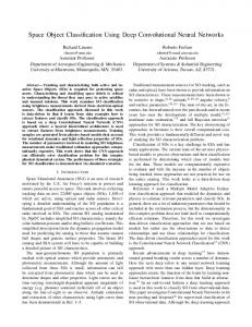
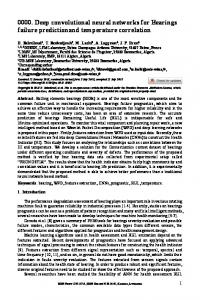
Those performances empirically show that CNNs are strong models to solve many music-related problems. Spectrograms match well with the assumption of CNNs from many perspectives. They are locally correlated, shift/translation invariances are often required, the output labels may depend on local, sparse features [8]. Fig. 1: Deconvolution results of CNNs trained for image classification. In each layer, the responses of the filters are shown on the left with gray backgrounds and the corresponding parts from images are shown on the right. Image is courtesy of [2].

behaviour of a CNN is not deterministic as the operation of max-pooling varies by input by input. This is why analysing the learnt weights of convolutional layers does not provide satisfying explanations. A way to understand a CNN is to visualise the features given different inputs. Visualisation of CNNs was introduced in [2], which showed how high-level features (postures/objects) are constructed by combining low-level features (lines/curves), as illustrated in Figure 1. In the figure, the shapes that features represent evolve. In the first layers, each feature simply responds to lines with different directions. By combining them, the features in the second and third layers can capture certain shapes - a circle, textures, honeycombs, etc. During this forward path, the features not only become more complex but also allow slight variances, and that is how the similar but different faces of dogs can be recognised by the same feature in Layer 5 in Figure 1. Finally, the features in the final layer successfully capture the outlines of the target objects such as cars, dogs, and human faces. Visualisation of CNNs helps not only to understand the process inside the black box model, but also to decide hyperparameters of the networks. For example, redundancy or deficiency of the capacity of the networks, which is limited by hyper-parameters such as the number of layers and filters, can be judged by inspecting the learnt filters. Network visualisation provides useful information since fine tuning hyperparameters is a crucial factor in obtaining cutting-edge performance.

3. AURALISATION OF LEARNT FILTERS Although we can obtain spectrograms by deconvolution, deconvolved spectrograms do not necessarily facilitate an intuitive explanation. This is because seeing a spectrogram does not necessarily provide clear intuition that is comparable to observing an image. To solve this problem, we propose to reconstruct audio signals from deconvolved spectrograms, which is called auralisation. This requires an additional stage for inversetransformation of a deconvolved spectrogram. The phase information is provided by the phase of the original timefrequency representations, following the generic approach in spectrogram-based sound source separation algorithms [9]. STFT is therefore recommended as it allows us to obtain a time-domain signal easily. Pseudo code of the auralisation is described in Listing 1. Line 1 indicates that we have a convolutional neural network that is trained for a target task. In line 2-4, an STFT representation of a music signal is provided. Line 5 computes the weights of the neural networks with the input STFT representation and the result is used during the deconvolution of the filters in line 6 ([2] for more details). Line 7-9 shows that the deconvolved filters can be converted into time-domain signals by applying the phase information and inverse STFT. 1 2 3 4 5 6 7 8 9

cnn_model = train_CNNs (* args ) # model src = load ( wavfile ) SRC = stft ( src ) aSRC , pSRC = SRC . mag , SRC . phase weights = unpool_info ( cnn_model , aSRC ) deconved_imgs = deconv ( weights , aSRC ) for img in deconved_imgs : signal = inverse_stft ( img * pSRC ) wav_write ( signal )

Listing 1: A pseudo-code of auralisation procedure

2.2. Audio and CNNs 4. EXPERIMENTS AND DISCUSSIONS Much research of CNNs on audio signal uses 2D timefrequency representations as input data. Various types of representations have been used including Short-time Fourier transform (STFT), Mel-spectrogram and constant-Q transform (CQT). CNNs show state-of-the-art performance on many tasks such as music structure segmentation[7], music tagging[6], and speech/music classification1 . 1 http://www.music-ir.org/mirex/wiki/2015:Music/Speech_ Classification_and_Detection_Results

We implemented a CNN-based genre classification algorithm using a dataset obtained from Naver Music 2 and based on Keras [10] and Theano [11]. All audio signal processing was done using librosa [12]. Three genres (ballad, dance, and hiphop) were classified using 8,000 songs in total. In order to maximally exploit the data, 10 clips of 4 seconds were extracted for each song, generating 80,000 data samples 2 http://music.naver.com,

a Korean music streaming service

Name Bach Dream Toy Eminem

Summary Classical, piano solo Pop, female vocal, piano, bass guitar Pop, male vocal, drums, piano, bass guitar Hiphop, male vocal, piano, drums, bass guitar

Table 2: Descriptions of the four selected music items

Bach Original

Dream

Toy

Eminem

Bach Dream Toy [Feature 1-9], Crude onset detector

Eminem

Bach Dream [Feature 1-27], Onset detector

Eminem

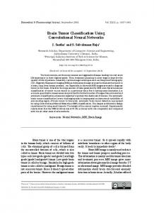
Fig. 2: Block diagram of the trained CNNs. Layer 1 2 3 4 5

Convolution 3×3 3×3 3×3 3×3 3×3

Effective width 93 ms 162 ms 302 ms 580 ms 1137 ms

Effective height 86 Hz 151 Hz 280 Hz 538 Hz 1270 Hz

Table 1: The effective sizes of convolutional kernels

by STFT. STFT is computed with 512-point windowed Fast Fourier Transform with 50% hop size and sampling rate of 11,025 Hz. 6,600/700/700 songs were designated as training/validation/test sets respectively. The CNN architecture consists of 5 convolutional layers of 64 feature maps and 3-by-3 convolution kernels, maxpooling with size and stride of (2,2), and two fully connected layers as illustrated in the figure 2. Dropout(0.5) is applied to the all convolutional and fully-connected layers to increases generalisation [13]. This system showed 75% of accuracy at the end of training. It is noteworthy that although a homogeneous size of convolutional kernels (3×3) are used, the effective coverages are increasing due to the subsampling, as in the table 1. We show two results in the following sections. In Section 4.1, the deconvolved spectrograms of selected learnt filters are presented with discussions. Section 4.2 shows how the learnt filters respond by the variations of key, chord, and instrument. 4.1. Deconvolved results with music excerpts We deconvolved and auralised the learnt features of Four music signals by Bach, Lena Park (Dream), Toy, and Eminem. Table 2 describes the items. In the following section, several selected examples of deconvolved spectrograms are illustrated with descriptions.3 The descriptions are not the designated goals but interpretations of the features. During the 3 The results are demonstrated on-line at http://wp.me/p5CDoD-k9. An example code of the deconvolution procedure is released at https: //github.com/keunwoochoi/Auralisation

Toy

Fig. 3: Spectrograms of deconvolved signal in Layer 1

overall process, listening to auralised signals helped to identify pattern in the learnt features. 4.1.1. Layer 1 0.15 0.00

(a) Feature 1-9

(b) Feature 1-27

0.15 0.25

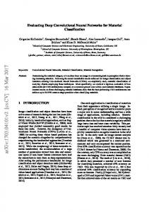
Fig. 4: The learnt weights of Features (a) 1-9 and (b) 1-27. The distributions along rows and columns roughly indicate high-pass filter behaviours along x-axis (time axis) and lowpass filter behaviours along y-axis (frequency axis). As a result, they behave as onset detectors. In Layer 1, we selected two features and present their deconvolved spectrograms as well as the corresponding weights. Because the weights in the first layer are applied to the input directly without max-pooling, the mechanism are determined and can be analysed by inspecting the weights regardless of input. For instance, Feature 1-9 (9th feature in Layer 1) and Feature 1-27, works as an onset detector. The learnt weights are shown in Figure 4. By inspecting the numbers, it can be

Bach Original

Dream

Toy

Eminem

Bach Original

Dream

Toy

Eminem

Bach Dream Toy [Feature 2-0], Good onset detector

Eminem

Bach Dream Toy [Feature 3-1], Better onset detector

Eminem

Bach Dream Toy [Feature 2-1], Bass note selector

Eminem

Bach Dream [Feature 3-7], Melody (top note)

Toy

Eminem

Bach Dream Toy [Feature 2-10], Harmonic selector

Eminem

Bach Dream Toy [Feature 3-38], Kick drum extractor

Eminem

Bach Dream Toy [Feature 2-48], Melody (large energy)

Eminem

Bach Dream Toy [Feature 3-40], Percussive eraser

Eminem



easily understood that the network learnt to capture vertical lines. In spectrograms, vertical lines often corresponds to the time-frequency signature of percussive instruments. Many other features showed similar behaviours in Layer 1. In other words, the features in Layer 1 learn to represent multiple onset detectors and suppressors with subtle differences. It is a similar result to the result that is often obtained in visual image recognition, where CNNs learn line detectors with various directions (also known as edge detectors), which are combined to create more complex shapes in the second layer. With spectrograms, the network focuses on detecting horizontal and vertical edges rather than diagonal edges. This may be explained by the energy distribution in spectrograms. Horizontal and vertical lines are main components of harmonic and percussive instruments, respectively, while diagonal lines mainly appear in the case of frequency modulation, which is relatively rare.

can be explained from two perspectives. First, as the features in Layer 2 can cover a wider range both in time and frequency axis than in layer 1, non-onset parts of signals can be suppressed more effectively. Second, the multiple onset detectors in Layer 1 can be combined, enhancing their effects. Feature 2-1 (bass note), roughly selects the lowest fundamental frequencies given harmonic patterns. Feature 210 behaves as a harmonic component selector, excluding the onset parts of the notes. Feature 2-48 is another harmonic component selector with subtle differences. It behaves as a short melodic fragments extractor, presumably by extracting the most salient harmonic components.

4.1.2. Layer 2 Layer 2 shows more evolved, complex features compared to Layer 1. Feature 2-0 is an advanced (or stricter) onset detectors than the onset detectors in Layer 1. This improvement

4.1.3. Layer 3 The patterns of some features in Layer 3 are similar to that of Layer 2. However, some of the features in Layer 3 contain higher-level information e.g. focusing on different instrument classes. The deconvolved signal from Feature 3-1 consists of onsets of harmonic instruments, being activated by voices and piano sounds but not highly activated by hi-hats and snares. The sustain and release parts of the envelopes are effectively

Toy

Eminem

Bach Original

Dream

Toy

Eminem

Bach Dream Toy [Feature 4-5], Lowest notes selector

Eminem

Bach Dream [Feature 5-11], texture 1

Toy

Eminem

Bach Dream Toy [Feature 4-11], Vertical line eraser

Eminem


Toy

Eminem

Bach Dream Toy [Feature 4-30], Long horizontal line selector

Eminem

Bach Dream Toy [Feature 5-56], Harmo-Rhythmic structure

Eminem


Eminem

Bach Original

Dream


filtered out in this feature. Feature 3-7 is similar to Feature 2-48 but it is more accurate at selecting the fundamental frequencies of top notes. Feature 3-38 extracts the sounds of kick drum with a very good audio quality. Feature 3-40 effectively suppresses transient parts, resulting softened signals. The learnt features imply that the roles of some learnt features are analogous to tasks such as harmonic-percussive separation, onset detection, and melody estimation.

4.1.4. Layer 4 Layer 4 is the second last layer of the convolutional layers in the architecture and expected to represent high-level features. In this layer, a convolutional kernel covers a large area (580 ms×538 Hz), which affects the deconvolved spectrograms. It becomes trickier to name the features by their characteristics, although their activation behaviours are still stable on input data. Feature 4-11 removes vertical lines and captures another harmonic texture. Although the coverages of the kernels increase, the features in Layer 4 try to find patterns more precisely rather than simply respond to common shapes such as edges. As a result, the activations become more sparse (local) because a feature responds only if a certain pattern – that matches the learnt features – exists, ignoring irrelevant patterns.

Toy

Fig. 8: Spectrograms of deconvolved signal in Layer 5 4.1.5. Layer 5 This is the final layer of the convolutional layers, and therefore it represents the highest-level features among all the learnt features. High-level features respond to latent and abstract concepts, which makes it more difficult to understand by either listening to auralised signals or seeing deconvolved spectrograms. Feature 5-11, 5-15, and 5-33 are therefore named as textures. Feature 5-56, harmo-rhythmic texture, is activated almost only if strong percussive instruments and harmonic patterns overlap. Feature 5-33 is completely inactivated with the fourth excerpt, which is the only Hip-Hop music, suggesting it may be useful for classification of HipHop. 4.2. Feature responses by attributes In this experiment, a set of model signals are created. Model signals are simplified music excerpts, each of which consists of a harmonic instrument playing various chords at different keys. In total, 7 instruments (pure sine, strings, acoustic guitar, saxophone, piano, electric guitar) × 8 chord types (intervals, major, minor, sus4, dominant7, major7, minor7, diminished) × 4 keys (Eb2, Bb2, A3, G4) are combined, resulting

frequency

time Fig. 9: A spectrogram of an example of the model signals – at the key of G4, an instrument of pure sine, and the chord of six major positions (first half) and six minor positions (second half). High-frequency ranges are trimmed for better frequency resolution.

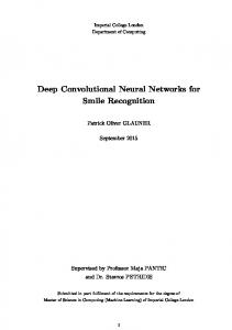
features in early layers are affected. However, the effect decreases as progressing towards deeper layers. At Layer 5, the chord pairs become more correlated then they do in the early layers, which means more robusness. The CNN is the most sensitive to the instrument variations at Layer 1. Considering the simple features in Layer 1, the different onset and harmonic patterns by instruments may contribute this. However, it becomes more robust in the deeper layer. At Layer 5, instruments are slightly less correlated than chords are. To summarise, all three variations show similar average correlations in Layer 5 , indicating the high-level features that CNN learnt to classifier genre are robust to the variations of key, chord, and instrument. 5. CONCLUSIONS

in 224 model signals. Figure 9 shows the spectrogram of one of the model signals. All the model signals are fed into the trained CNN. Then, all the learnt features are deconvolved, resulting in 64 spectrograms per layer and per model signal. In other words, there are 224 spectrograms for each feature. If we compute the average correlation of the 6 pairs of keys ({Eb2, Bb2}, {Eb2, A3}, {Eb2, G4}, {Bb2, A3}, {Bb2, G4}, {A3, G4}) from the features in Layer 1 with fixing the chord and instrument, we can see how sensitive (or not robust) the CNN is to key changes in Layer 1. The robustness of the other layers and to chord or instrument can be computed in the same manner. We computed the average of this correlation for all features, every pairs of key, chord, and instrument, and per layer. The result is plotted in Figure 10. According to Figure 10, key variations have the smallest effect on the CNN for genre classification over the whole network. It agrees well with general understanding of genre, in which key does not play an important role. The low correlation with chord type variations in Layer 1 indicates the

1.0

Avg. correlation of every pair in each layer

correlation

0.8

key chord instrument

0.6 0.4 0.2 0.0

original 1

2

3

4

5

layer number

Fig. 10: Average correlation of every pairs in each layer by the variations of key, chord, and instrument. Error bars refer to the corresponding standard deviations.

We introduced auralisation of CNNs, which is an extension of CNNs visualisation. This is done by inverse-transformation of deconvolved spectrograms to obtain time-domain audio signals. Listening to the audio signal enables researchers to understand the mechanism of CNNs that are trained with audio signals. In the experiments, we trained a 5-layer CNN to classify genres. Selected learnt features are reported with interpretations from musical and music information aspects. The comparison of correlations of feature responses showed how the features evolve and become more invariant to the chord and instrument variations. Further research will include computational analysis of learnt features. 6. REFERENCES [1] Keunwoo Choi, George Fazekas, Mark Sandler, and Jeonghee Kim, “Auralisation of deep convolutional neural networks: Listening to learned features,” ISMIR latebreaking session, 2015. [2] Matthew D Zeiler and Rob Fergus, “Visualizing and understanding convolutional networks,” in Computer Vision–ECCV 2014, pp. 818–833. Springer, 2014. [3] Alex Krizhevsky, Ilya Sutskever, and Geoffrey E Hinton, “Imagenet classification with deep convolutional neural networks,” in Advances in neural information processing systems, 2012, pp. 1097–1105. [4] Taejin Park and Taejin Lee, “Music-noise segmentation in spectrotemporal domain using convolutional neural networks,” ISMIR late-breaking session, 2015. [5] Eric J Humphrey and Juan P Bello, “Rethinking automatic chord recognition with convolutional neural networks,” in Machine Learning and Applications (ICMLA), International Conference on. IEEE, 2012. [6] Sander Dieleman and Benjamin Schrauwen, “End-toend learning for music audio,” in Acoustics, Speech and

Signal Processing (ICASSP), 2014 IEEE International Conference on. IEEE, 2014, pp. 6964–6968. [7] Karen Ullrich, Jan Schlüter, and Thomas Grill, “Boundary detection in music structure analysis using convolutional neural networks,” in Proceedings of the 15th International Society for Music Information Retrieval Conference (ISMIR 2014), Taipei, Taiwan, 2014. [8] Yann LeCun and M Ranzato, “Deep learning tutorial,” in Tutorials in International Conference on Machine Learning (ICML13), Citeseer. Citeseer, 2013. [9] Derry Fitzgerald and Rajesh Jaiswal, “On the use of masking filters in sound source separation,” Int. Conference on Digital Audio Effects (DAFx-12), 2012. [10] François Chollet, “Keras: Deep learning library for theano and tensorflow,” https://github.com/fchollet/keras, 2015. [11] Theano Development Team, “Theano: A Python framework for fast computation of mathematical expressions,” arXiv e-prints, vol. abs/1605.02688, May 2016. [12] Brian McFee, Colin Raffel, Dawen Liang, Daniel PW Ellis, Matt McVicar, Eric Battenberg, and Oriol Nieto, “librosa: Audio and music signal analysis in python,” in Proceedings of the 14th Python in Science Conference, 2015. [13] Nitish Srivastava, Geoffrey Hinton, Alex Krizhevsky, Ilya Sutskever, and Ruslan Salakhutdinov, “Dropout: A simple way to prevent neural networks from overfitting,” The Journal of Machine Learning Research, vol. 15, no. 1, pp. 1929–1958, 2014.