Exploring the Relationship between Remotely-Sensed ... - OpenPub

International Journal of

Geo-Information Article

Exploring the Relationship between Remotely-Sensed Spectral Variables and Attributes of Tropical Forest Vegetation under the Influence of Local Forest Institutions Shivani Agarwal 1,2, *, Duccio Rocchini 3 , Aniruddha Marathe 1,2 and Harini Nagendra 4 1 2 3 4

*

Ashoka Trust for Research in Ecology and the Environment, Royal Enclave, Srirampura, Jakkur, Bangalore 560064, India; [email protected] Manipal University, Manipal, Udupi 576 104, India Fondazione Edmund Mach, Research and Innovation Centre, Department Biodiversity and Molecular Ecology, 38010 S. Michele All’adige (Trento), Italy; [email protected] or [email protected] Azim Premji University, PES Institute of Technology Campus, Pixel Park, B Block, Electronics City, Beside Nice Road, Hosur Road, Bengaluru 560 100, India; [email protected] Correspondence: [email protected] or [email protected]; Tel.: +91-767-644-5031

Academic Editor: Wolfgang Kainz Received: 25 April 2016; Accepted: 11 July 2016; Published: 14 July 2016

Abstract: Conservation of forests outside protected areas is essential for maintaining forest connectivity, which largely depends on the effectiveness of local institutions. In this study, we use Landsat data to explore the relationship between vegetation structure and forest management institutions, in order to assess the efficacy of local institutions in management of forests outside protected areas. These forests form part of an important tiger corridor in Eastern Maharashtra, India. We assessed forest condition using 450 randomly placed 10 m radius circular plots in forest patches of villages with and without local institutions, to understand the impact of these institutions on forest vegetation. Tree density and species richness were significantly different between villages with and without local forest institutions, but there was no difference in tree biomass. We also found a significant difference in the relationship between tree density and NDVI between villages with and without local forest institutions. However, the relationship between species richness and NDVI did not differ significantly. The methods proposed by this study evaluate the status of forest management in a forest corridor using remotely sensed data and could be effectively used to identify the extent of vegetation health and management status. Keywords: biodiversity; quantile regression; remote sensing; tree biodiversity

1. Introduction Ecological research is vital for establishing effective management and conservation policies for the proper governance of natural resources [1]. In particular, evidence-based data on the effectiveness of conservation management typically requires a solid foundation of in-depth fieldwork. Although this is very important, field data collection is a time-consuming and expensive process [2]. It can often be very difficult to acquire field data in remote and inaccessible places, in areas with challenging terrain, or in areas of ongoing conflict and turmoil that may be of high ecological importance. Remote sensing can be a valuable aid in such contexts. Remote sensing studies are conducted with the aid of satellite images whereas ecological studies involve in-depth field work, which may or may not cover large spatial regions [2]. Predictions based solely on ecological field studies are hence spatially bounded, and often need to be complemented with broad-scale geographic data for extrapolation to

ISPRS Int. J. Geo-Inf. 2016, 5, 117; doi:10.3390/ijgi5070117

www.mdpi.com/journal/ijgi

ISPRS Int. J. Geo-Inf. 2016, 5, 117

2 of 16

the landscape or regional scale [3]. A combination of remote sensing and field-based ecology research has contributed immensely towards understanding ecological processes, since they facilitate research at moderate to large spatial extents in a cost-effective manner [4,5]. Although ecological field based research is not replaceable by remote sensing methods, the two methods complement each other for better understanding of ecological processes. This can further be incorporated in conservation and management plans [6]. Ecological variability (heterogeneity and biodiversity) forms an important indicator of ecosystem function and ecosystem health [7]. Several studies have been carried out to find the relationship between remotely sensed spectral heterogeneity and ecological variability [8,9]. The Normalized Difference Vegetation Index (NDVI) and other vegetation indices have frequently been used as proxies for vegetation health and structure [10–12]. Recent studies have also demonstrated the potential for spectral heterogeneity to be used as a proxy for alpha and beta-diversity of an area, helping in the characterization of biodiversity at larger spatial scales [8,13]. However, ecological processes are complex and the relationship with spectral data may not be very straightforward. For example, it is very difficult to assess understory vegetation variability through optical remote sensing, as such images typically capture information largely from the upper canopy. Active remote sensing such as LiDAR (Light Detection And Ranging) technology could provide solutions to this challenge [14] but typically, such images are expensive and often difficult to acquire, particularly in many biodiverse tropical environments [15]. Thus, so far, most studies have been based on moderate resolution images such as the Landsat data archive, which is freely available [16]. Vegetation structure and variability arises not only as a consequence of ecological and bio-physical processes but is also shaped by social, economic and institutional processes [17–19]. Studies from Europe have shown that the species richness, number of dead logs and soil nitrogen are higher in unmanaged forest patches compared to managed forest patches and that the forest patches differ in forest structural stages such as understory growth [20,21]. Institutional processes play an important role in impacting vegetation structure and variability, such as management of forest patches within as well as outside protected areas [22,23]. In this context, most research addressing the impact of institutions on forest biodiversity and variability has focused on state-administered protected areas [24–26]. Globally, a large extent of forests lies outside protected areas and is managed by various institutional structures. Local community institutions play an important role in maintaining these forest patches [27]. India harbours large, connected forest areas with high plant and animal diversity. A large proportion of India’s forest land is located outside the country’s protected area network [25,28]. Legally, forest patches outside protected areas belong to the state. These forest patches are under the formal control of the Indian Forest Department, but at smaller scales may be managed by local communities through informal institutions such as sacred groves, as well as by traditional norms of local communities that relate to hunting and harvesting of forest resources [29]. Recently, through Joint Forest Management and the Indian Forest Rights Act of 2006, local communities have also received some de jure (formal) rights to access and maintain forest patches [22,30]. However, forests outside protected areas are undergoing rapid changes, given their location in densely populated landscapes and face economic and political pressure [25,28,31]. Conservation of these forest patches is very important for social reasons such as livelihood dependence of local communities, as well as ecological reasons including wildlife protection. So far, remotely sensed data has been widely used to classify different types of forest and to assess changes in the forest density, diversity and distribution [4,32]. However, understanding the role of local institutions with the aid of remote sensing is comparatively less explored. In this study, we attempt to develop a better understanding of the relationship between spectral and ecological variability under the influence of local institutions. This can help in extrapolating the relationship between institution and vegetation to the regional level so as to provide policy inputs. The location of this research is in a forest corridor that connects important protected areas such as the Pench Tiger Reserve and the Tadoba-Andhari Tiger Reserve, among several others, within the eastern Maharashtra region. We focus on the forest outside the tiger reserves that are potential corridors



3 of 16

3 of 16

for biodiversity [33]. In this landscape, forest patches are managed by diverse institutional settings that range from active involvement local communities forest management, co-management that range from active involvement of of local communities in in forest management, to to co-management local communities and forest department, and management entirely forest department, byby local communities and thethe forest department, and management entirely by by thethe forest department, without any participation from local communities. Several common property resource studies have without any participation from local communities. Several common property resource studies have shown that there is a need for local participation in order to achieve larger conservation goals [34–37]. shown that there is a need for local participation in order to achieve larger conservation goals [34–37]. Previous research this region argued that community institutions important protection Previous research in in this region hashas argued that community institutions areare important forfor protection outside protected areas [37]. However, there has been limited assessment of this hypothesis. outside protected areas [37]. However, there has been limited assessment of this hypothesis. study, we use Landsat to understand the between relationship between spectral In In thisthis study, we use Landsat imagery imagery to understand the relationship spectral heterogeneity heterogeneity and vegetation variability in the presence or absence of local institutions. and vegetation variability in the presence or absence of local institutions. The specific objectives are: The specific objectives are:

1. 1. To To explore thethe relationship between remotely-sensed spectral variables such as as thethe NDVI, and explore relationship between remotely-sensed spectral variables such NDVI, and attributes of forest vegetation, in particular of species richness, tree density, and biomass. attributes of forest vegetation, in particular of species richness, tree density, and biomass. 2. 2. To To investigate how management by by local (community) institutions influences vegetation diversity. investigate how management local (community) institutions influences vegetation diversity. 3. 3. To To examine whether the relationship between remotely-sensed spectral variables and attributes examine whether the relationship between remotely-sensed spectral variables and attributes of of forest vegetation diversity differ in in forests managed with and without thethe participation of of forest vegetation diversity differ forests managed with and without participation local communities. local communities. 2. Material andand Methods 2. Material Methods Study Area 2.1.2.1. Study Area This study was carried in five forest divisions in Eastern Maharashtra, collectively known This study was carried outout in five forest divisions in Eastern Maharashtra, collectively known as as “Vidarbha” (Figure 1). Vidarbha is an underdeveloped region within the state of Maharashtra that “Vidarbha” (Figure 1). Vidarbha is an underdeveloped region within the state of Maharashtra that has has rich dry tropical forestand cover high population density. are nine protected in the rich dry tropical forest cover highand population density. There areThere nine protected areas in theareas selected selected region with two Tiger Reserves, six Wildlife Sanctuaries and one National Park (Figure region with two Tiger Reserves, six Wildlife Sanctuaries and one National Park (Figure 1). Total area 1). 2, out of11,000 2 Totalforest area cover underinforest cover in the eight forest divisions is around km2 ,around out of which only under the eight forest divisions is around 11,000 km which only 1350 km 2 around 1350 kmprotected is covered by the areas. Themaintains forest department maintains forests areas outside is covered by the areas. Theprotected forest department the forests outside the protected protected areas according to categories such as Reserve Forest and Protected Forest. At times, these according to categories such as Reserve Forest and Protected Forest. At times, these are also handedare also over to the ForestCorporation Development Maharashtra for(Table management (Table 1). over tohanded the Forest Development ofCorporation Maharashtraoffor management 1).

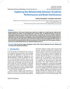
Figure 1. Study area depicting thethe distribution ofofprotected Figure 1. Study area depicting distribution protectedareas areasininthe thestudy studyarea, area,and and the the locations locations of of 15 15 surveyed surveyed villages. villages.


4 of 16

Table 1. Types of forest management regimes outside protected areas, with a description of rules governing use and access to forest products. Different Types of Management Regimes

Rules

Reserve Forest (RF)

RF patches are legally government property, and under control of government officials. Within RFs, plantation, beat cutting (cut down trees based on predetermined range of DBH in the selected coupe/beat for plantation) and other forestry practices are conducted according to 5 year plans of the forest department. There are restrictions on logging and hunting. Local residents can collect fuelwood only through head-loads. Taking bullock-carts, bicycles and axes for wood collection is prohibited.

Forest Development Corporation of Maharashtra (FDCM)

Some RF compartments are leased to the Forest Development Corporation of Maharashtra for afforestation and timber extraction and sale. Local community work in FDCM forests for daily wages is permitted, but workers are not allowed to access forest resources for their livelihood. They are sometimes allowed to use resources that are not commercially useful for the FDCM department.

Protected Forest (PF)

PFs are similar to RFs; however, there are fewer restrictions on village residents in terms of using the former as compared to the latter. The term PF is sometimes interchangeably used with village forest. Village residents are allowed to collect fuelwood, timber and other NTFPs.

Community Forest Management (CFM)

Some patches of RFs and PFs are informally managed by local communities, who formulate rules and regulations on use and management. Some of these community associations later received formal recognition through Joint Forest Management (JFM), with forest patches continuing to be managed by the local community but with limited authority, under the overall control of the Forest Department. Recently, some local communities have claimed rights over forest patches through the Community Forest Rights section of the Forest Rights Act (FRA).


5 of 16

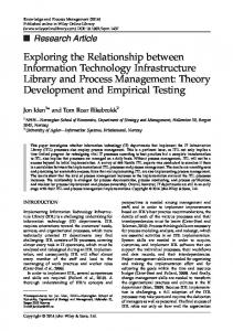
Approximately thirty-three percent of the population [38] belongs to tribal communities and lives in close proximity to the forest. The tribal as well as non-tribal communities are highly dependent on forests for subsistence and economic livelihoods. Thus, it is very important to understand the interface between local communities, forest use, and conservation of the forest corridor in this region [39]. At the village level, the communities have informally devised rules and regulations for harvesting, managing and protecting the forest resources. At the same time, initiatives of the state such as Joint Forest Management (JFM) schemes and the Forest Rights Act provide limited recognition of rights to local communities for utilization and management of forest patches in their vicinity. Understanding the interplay between these institutions and extent of vegetation within this corridor is very important for maintaining a viable wildlife population. Remote sensing methods provide considerable assistance for covering a regional scale of study. 2.2. Field Data Collection Fieldwork was carried out from October 2013 to February 2014 (during winter), in eight forest divisions (administrative categories) namely Nagpur, Bhandara, Gondia, Brahmapuri, Wadsa, Gadchiroli, Chandrapur buffer and Chandrapur non-buffer. In order to separately manage some forests within the buffer region of Tadoba-Andhari Tiger Reserve (TATR) under the eco-development policy, the Chandrapur forest division was recently divided into buffer and non-buffer forest divisions. Two villages were selected in each of the eight forest divisions. The snowball sampling method was used to gather information from forest department officials, local NGOs and other key informants regarding local forest institutions. In order to focus on institutional effects, we purposefully selected the villages in such a way that they were similar in terms of population, distance to forest, proximity to market and town, and other facilities. In villages where we found the active participation of local residents in forest management, or where there was joint action by local residents and the forest department in monitoring/managing the forest resource, institutions were categorized as ‘Present’. In villages where peoples’ participation was lacking, either due to the dominance of management by the forest department or with no management of forest resources either by people or by the forest department, institutions were categorized as ‘Absent’. As the Chandrapur Buffer Forest Division has no village without local forest institutions, we have selected 15 villages for this study. Involvement of local people in forest management was subjective and we needed thorough information. Therefore, snowball and purposive sampling methods were used to identify the villages. Within each of the selected 15 villages, tree density, species richness and tree biomass were estimated using 30 circular forest plots (i.e., a total of 450 plots across the study area) of 10 m radius, within which smaller nested circular plots of 3 m and 1 m radii were used to assess sapling and seedling density and diversity (Figure 2). To select the location of the circular plots, the forest boundaries of each village were mapped and divided into 60 m ˆ 60 m grids, so that the plots were at least be 60 m or two pixels (in case of Landsat image) apart from each other. Then, we randomly selected the 30 grids using the vector tool operation of QGIS [40]. We located each plot in the field by tracking the centroid of each selected grid using a GPS device (GARMIN eTrex Vista, Olathe, KS, USA). We laid circular plots by measuring 10 m radii around the centroid. The projection used was the geographic latitude/longitude World Geodetic System 1984 (WGS84). In 10 m circular plots, the GBH (Girth at Breast Height) and height of all trees, shrubs and climber species were recorded for all individuals with GBH of more than 10 cm. In 3 m circular plots, the GBH and height of all trees, shrubs, and climber species were recorded for all individuals with GBH less than 10 cm and height more than 1 m. In 1 m circular plots, species identity was recorded for all trees, shrubs, climber species, and herb individuals with height less than 1 m. Later, DBH (Diameter at Breast height) was calculated using GBH. In order to avoid seasonal variation that mostly affects shrub and herb species composition, the data was collected in winter across all villages. We calculated the tree density, species richness and biomass for each plot. The biomass was calculated using the formula provided by Chave et al. [41], which accounts for tree taper and in which


6 of 16


6 of 16

wood density is multiplied by the volume of the cylinder. Wood density data were obtained from wood density multiplied by the volume the cylinder. Wood density data obtained from Zanne et al. [42]isand the Ecosystems Ecologyoflaboratory of the National Centre forwere Biological Sciences Zanne etBangalore, al. [42] andIndia. the Ecosystems Ecology laboratory of the National Centre for Biological Sciences (NCBS), (NCBS), Bangalore, India.

Figure 2. Circular plot method forfor sampling tree, sapling and seedling in in each surveyed village. Figure 2. Circular plot method sampling tree, sapling and seedling each surveyed village.

2.3. Remotely Remotely Sensed Sensed Data Data 2.3. Landsat 88 surface surface reflectance reflectance imagery imagery with with aa spatial spatial resolution resolution of of 30 30 m, m, of of 14th 14th December December 2013 2013 Landsat acquisition date date were were downloaded downloaded from from the the USGS USGS website, website, to to assess assess the the relationship between spectral spectral acquisition relationship between value and vegetation variability across different sites. This time frame corresponds with the winter value and vegetation variability across different sites. This time frame corresponds with the winter time frame (October–February) during which field data was collected. The size of each plot i.e., 10 m m time frame (October–February) during which field data was collected. The size of each plot i.e., 10 radius circular circular plot plot is is less less than than the the pixel pixel size size of of 30 30 m m resolution resolution of of Landsat Landsat 88 images. images. In In order order to to radius account for the positional error of around 5–8 m radius, a 3 × 3 pixel window around the central pixel account for the positional error of around 5–8 m radius, a 3 ˆ 3 pixel window around the central pixel of plot, plot, location location was was used used to to calculate of calculate the the mean mean and and standard standard deviation deviation of of selected selected indices indices and and bands. bands. This method was used to extract value for Tasseled Cap indices for wetness [43], NDVI and standard This method was used to extract value for Tasseled Cap indices for wetness [43], NDVI and standard deviation of of NDVI NDVI (SD-NDVI). (SD-NDVI). NDVI NDVI is is derived derived from from red red and and infrared infrared bands. bands. NDVI NDVI values values range range deviation between ´1 −1 to vegetation. Image processing software, software, ERDAS ERDAS between to +1, +1, where where high high values values indicate indicate greener greener vegetation. Image processing Imagine™ (9.2, ERDAS Inc., Norcross, GA, USA) was used to calculate NDVI and SD-NDVI; and Imagine™ (9.2, ERDAS Inc., Norcross, GA, USA) was used to calculate NDVI and SD-NDVI; and GRASS GIS 7.0.0RC2 (GRASS Development Team, Michele all'Adige, Italy) was used for Tasseled Cap GRASS GIS 7.0.0RC2 (GRASS Development Team, Michele all'Adige, Italy) was used for Tasseled Cap indices for for Wetness. Wetness. indices 2.4. Data Data Analysis Analysis 2.4. We used used quantile quantile regression regressionat atvery veryhigh high quantile quantilevalues values (tau (tau == 0.95) 0.95) to to describe describe the the relationship relationship We between NDVI and tree density at plots. NDVI is a measure of greenness (or absorption of solar solar between NDVI and tree density at plots. NDVI is a measure of greenness (or absorption of radiation by by chlorophyll) chlorophyll) and and is is naturally naturally correlated correlated with with the the live live vegetation vegetation cover. cover. This This may may include include radiation any form of vegetation such as grasses, shrubs, or trees. Therefore, the value of NDVI is not limited any form of vegetation such as grasses, shrubs, or trees. Therefore, the value of NDVI is not limited by tree tree density density alone. alone. In In such such aa case, case, ordinary ordinary least least squares squares regression regression that that describes describes the the relationship relationship by between mean mean of of tree tree density density and and NDVI NDVI is is not not appropriate. appropriate. By fitting regression regression only only to to higher higher between By fitting quantiles of the data, we restrict the prediction to the slice of the data where most NDVI is contributed quantiles of the data, we restrict the prediction to the slice of the data where most NDVI is contributed by standing standing tree treevegetation. vegetation.Quantile Quantileregression regressionisisextensively extensivelyused usedininvarious various ecological studies, by ecological studies, asas it it helps in estimating the functional relationship between the variables at different quantile values helps in estimating the functional relationship between the variables at different quantile values [13,44–46]. [13,44–46]. Instudies, ecological it is very all thecausing variables an effect, and In ecological it isstudies, very difficult to difficult measureto allmeasure the variables ancausing effect, and threshold threshold values are often better described than total variation. Therefore, estimating multiple regression slopes at different quantiles provides greater understanding as compared to ordinary least squares regression [44].

ISPRS J. Geo-Inf.2016, 2016,5,5,117 117 ISPRS Int.Int. J. Geo-Inf.

7 of716 of 16

The eight forest divisions within which the villages were present had identical modes of operation values arenot often better described than total variation. Therefore, estimating multiple regression and did have any specific differences in the policies they were implementing. Therefore, while the villages were quantiles nested within forest greater divisions, we did not expect this to have an effect in addition slopes at different provides understanding as compared to ordinary least squares to local conditions. To confirm this assumption we compared tree density, species richness and tree regression [44]. biomass of between villages within forest divisionwere using Mann–Whitney U test (Table In The eight forest divisions within each which the villages present had identical modes of A1). operation addition, also compared same variables betweenthey villages, and without institutions, butthe and did notwe have any specific the differences in the policies werewith implementing. Therefore, while pooledwere across all forest divisions. We expected localtoinstitutions should be consistent villages nested within forest divisions, we that did the not effect expectofthis have an effect in addition to local between these two comparisons. conditions. To confirm this assumption we compared tree density, species richness and tree biomass We compared the relationship between spectral and plant community between of between villages within each forest division using Mann–Whitney U testdata (Table A1). Invillages addition, with and without institutions using regression at a high quantile (0.95). As spectral heterogeneity is we also compared the same variables between villages, with and without institutions, but pooled a good proxy for beta diversity [46], we also compared the relationship between spectral dissimilarity across all forest divisions. We expected that the effect of local institutions should be consistent between and beta-diversity in the institution and non-institution villages. The analysis was performed in R 3.2.2 these two comparisons. (R Core Team, Vienna, Austria) using package “quantreg version 5.11” for quantile regression [47] and We compared the relationship between spectral and plant community data between villages with package “vegan version 2.3-1” [48] for dissimilarity indices. and without institutions using regression at a high quantile (0.95). As spectral heterogeneity is a good proxy for beta diversity [46], we also compared the relationship between spectral dissimilarity and 3. Results beta-diversity in the institution and non-institution villages. The analysis was performed in R 3.2.2 (R3.1. Core Team, Vienna, Austria) using and package “quantreg Relationship between Plant Species Spectral Diversityversion 5.11” for quantile regression [47] and package “vegan version 2.3-1” [48] for dissimilarity indices. Tree density and richness showed a clear positive relationship with spectral indices and negative relationship with spectral heterogeneity, while the relationship between biomass and the spectral 3. Results indices was much weaker in both cases. Variance of the response variables also increased with the spectral indices. This isPlant most Species likely due the nature of the relationship between spectral indices and 3.1. Relationship between andtoSpectral Diversity tree vegetation (Figure 3). Tree density and richness showed clear positive relationshiprelated with spectral indices andinnegative Tree density, species richness, anda biomass were significantly to spectral values both relationship with spectral heterogeneity, while the relationship between biomass and the spectral quantile and linear regression. Estimates of intercept took more extreme values (positive and negative), indices was much weakerininquantile both cases. Variance of the to response variables Thus, also increased with the and slopes were steeper regression compared linear regression. the relationship spectral indices. Thisofisvegetation most likelyand duespectral to the nature the relationship between spectral indices between attributes indices of varies with the quantile value, and the higherand tree vegetation 3). effect than the mean (Figure 3 and Table 2). quantiles have(Figure a stronger

Figure 3. Relationship between tree density (no. of trees/ha), species richness and biomass (kg) with NDVI, SD–NDVI and wetness using quantile regression (0.95 tau) and linear regression. The dashed line is for linear regression and solid line is for quantile regression (0.95 tau).


8 of 16

Tree density, species richness, and biomass were significantly related to spectral values in both ISPRS Int. J. Geo-Inf. 5, 117 8 of 16 quantile and linear2016, regression. Estimates of intercept took more extreme values (positive and negative), and slopes were steeper in quantile regression compared to linear regression. Thus, the relationship Figure 3. Relationship between tree density (no. of trees/ha), species richness and biomass (kg) with between attributes of vegetation and spectral indices varies with the quantile value, and the higher NDVI, SD–NDVI and wetness using quantile regression (0.95 tau) and linear regression. The dashed quantiles have a stronger effect than the mean (Figure 3 and Table 2). line is for linear regression and solid line is for quantile regression (0.95 tau).

Table 2. Comparison of the results of quantile regression (0.95 tau) and linear regression for the Table 2. Comparison of the results of quantile regression (0.95 tau) and linear regression for the relationship ofof tree with NDVI, NDVI,SD–NDVI SD–NDVIand andwetness. wetness. relationship treedensity, density,species speciesrichness richnessand and biomass biomass with Variable Variable

Tree density Tree density

Species richness

Tree Tree biomass biomass

Parameter Parameter Intercept: NDVI Intercept: NDVI Slope: NDVI Slope: NDVI Intercept: SD–NDVI Intercept: SD–NDVI Slope:SD–NDVI SD–NDVI Slope: Intercept:Wetness Wetness Intercept: Slope:Wetness Wetness Slope: Intercept:NDVI NDVI Intercept: Slope:NDVI NDVI Slope: Intercept: Intercept:SD–NDVI SD–NDVI Slope: Slope:SD–NDVI SD–NDVI Intercept: Intercept:Wetness Wetness Slope: Wetness Slope: Wetness Intercept: Intercept:NDVI NDVI Slope: Slope:NDVI NDVI Intercept: SD–NDVI Intercept: SD–NDVI Slope: SD–NDVI Slope: SD–NDVI Intercept: Wetness Intercept: Wetness Slope: Wetness Slope: Wetness

Quantile Regression (tau = 0.95) Quantile Regression (tau = 0.95) Estimate p Value Estimate p Value −4.68 (±7.9) 0.55 ´4.68 (˘7.9) 0.55 97.97 (±11.29)