Mar 9, 2009 - with an emphasis on the themes relevant to our proposed procedure for model ... Elegant recent results by several authors [8], [24], [25] have ...... matrices,â July 2007. http://terrytao.wordpress.com/2007/07/02/open-question-.
IEEE TRANSACTIONS ON SIGNAL PROCESSING
1
Fast Bayesian Matching Pursuit: Model Uncertainty and Parameter Estimation for Sparse Linear Models Philip Schniter Senior Member, IEEE, Lee C. Potter, Senior Member, IEEE and Justin Ziniel
Abstract A low-complexity recursive procedure is presented for model selection and minimum mean squared error (MMSE) estimation in linear regression. Emphasis is given to the case of a sparse parameter vector and fewer observations than unknown parameters. A Gaussian mixture is chosen as the prior on the unknown parameter vector. The algorithm returns both a set of high posterior probability models and an approximate MMSE estimate of the parameter vector. Exact ratios of posterior probabilities serve to reveal potential ambiguity among multiple candidate solutions that are ambiguous due to observation noise or correlation among columns in the regressor matrix. Algorithm complexity is O(M N K), with M observations, N coefficients, and K nonzero coefficients. For the case that hyperparameters are unknown, an approximate maximum likelihood estimator is proposed based on the generalized expectationmaximization algorithm. Numerical simulations demonstrate estimation performance and illustrate the distinctions between MMSE estimation and maximum a posteriori probability model selection.
Index Terms Sparse reconstruction, compressive sampling, compressed sensing, sparse linear regression, Bayesian model averaging, Bayesian variable selection, empirical Bayes.
Manuscript submitted September 9, 2008 and revised March 9, 2009. This investigation was supported by National Science Foundation Grant 0237037, Office of Naval Research grant N00014-07-1-0209, and AFOSR award FA9550-06-1-0324. A preliminary version of this work was presented at the Workshop on Information Theory and Applications (ITA), La Jolla, CA, January 2008. The authors are with the Department of Electrical and Computer Engineering, The Ohio State University, Columbus, OH, 43210-1272.
March 9, 2009
DRAFT
IEEE TRANSACTIONS ON SIGNAL PROCESSING
2
I. I NTRODUCTION Sparse linear regression is a topic of long-standing interest in signal processing, statistics, and geophysics. The linear model is given by y = Ax + w,
(1)
with observation vector y , known regressor matrix A, unknown coefficients x, and additive noise w. In sparse problems, the prior belief is that only a small fraction of coefficients are non-negligible. We adopt a Bayesian approach, which we now review in general terms. Let γk denote a candidate model, with k indexing the countably many models under consideration. A prior probability p(γk ) is assigned to each model, and a prior p(θ k |γk ) is adopted for the parameters of each model. For example, in (1) a model γk might indicate which entries in x ∈ RN are nonzero, resulting in 2N candidate models. For linear regression, a model is also known as a variable selection or basis selection. Margining out parameters and conditioning on the observations yields posterior model probabilities p(y|γk )p(γk ) p(γk |y) = P . j p(y|γj )p(γj )
(2)
Pairwise comparison of candidate models is given by the posterior odds p(γk |y) p(y|γk ) p(γk ) = . p(γj |y) p(y|γj ) p(γj )
(3)
The model posterior probabilities give a full description of the post-data uncertainty and are useful for inference and decision tasks. A common choice is to compute a single model that maximizes the posterior probability—the MAP estimate, γˆ⋆ . However, to obtain the minimum mean squared error estimate of x, one must compute a weighted average of conditional mean estimates over all models with nonzero probability, ˆ mmse = x
X
p(γk |y) E{x|y, γk }.
(4)
k
Bayesian model averaging (e.g., [1], [2] and references therein) is a name sometimes given to this incorporation of model uncertainty and stands in contrast to model selection, which is the report of a single model. Thus, the essential element provided by the Bayesian approach is the quantification of posterior model uncertainty. The posterior odds reveal uncertainty among multiple candidate solutions that are ambiguous due to observation noise or correlation among columns in the regressor matrix, A. Bayesian techniques are classical; the novelty here is a suite of computational techniques that make Bayesian estimation not only tractable, but low complexity, for the sparse linear model, with emphasis on the case of fewer observations than unknown variables. March 9, 2009
DRAFT
IEEE TRANSACTIONS ON SIGNAL PROCESSING
3
This manuscript is organized as follows. In Section II we briefly survey existing approaches to sparse linear regression. In Section III, we state a flexible signal model and priors for sparse signals; the priors explicitly specify our modeling assumptions and admit precise interpretation. In Section IV, we describe our proposed algorithm. A tree-search is combined with a low-complexity update of model posterior probabilities to find a dominant set of likely models. An algorithm for computing approximate maximum likelihood estimates of the hyperparameters, based on a generalized expectation maximization (EM) update, is presented in Section V for use when such hyperparameters are not known for a given application. We numerically investigate in Section VI the algorithm’s performance. In Section VII, we give specific comparison to related work. Conclusions are summarized in Section VIII. II. T ECHNIQUES
FOR
S PARSE L INEAR R EGRESSION
We present a brief and necessarily incomplete survey of existing approaches to sparse linear regression, with an emphasis on the themes relevant to our proposed procedure for model uncertainty and parameter estimation. For convenience, we coarsely partition approaches into those that do or do not explicitly adopt prior distributions. A. Algorithms for sparse signal reconstruction In sparse signal reconstruction, the general aim is to identify the smallest subset of columns of the regressor matrix, A, whose linear span contains (approximately) the observations, y . Algorithmic approaches have been proposed for several decades and broadly fall into three categories. The algorithms return a single model estimate and do not quantify uncertainty in the reported estimate. The algorithms have typically been developed without recourse to probabilistic priors. One class of algorithms adopts a greedy search heuristic. Examples include CLEAN [3], projection pursuit [4], and orthogonal matching pursuit (OMP) [5]. There exist sufficient conditions [6], [7] on the sparseness of x and singular values of subsets of columns of A (e.g., the restricted isometry property [8]) such that a regularized OMP stably recovers x with high probability. A second class of algorithms recursively solves a sequence of iteratively re-weighted linear leastsquares (IRLS) problems [9]–[11]; recent results [12] for the noiseless case have established sufficient conditions such that the sequence converges to the sparsest solution. A third class comprises penalized least-squares solutions for x and has likewise been used for at least four decades [13]. In this class of approaches, parameters are found via the optimization ˆ = argmin kAx − yk22 + τ kxkpp , x
(5)
x
March 9, 2009
DRAFT
IEEE TRANSACTIONS ON SIGNAL PROCESSING
4
or, equivalently, for some ǫ > 0 ˆ = argmin kxkp s.t. kAx − yk22 < ǫ. x
(6)
x
Ridge regression [14] (i.e., Tikhonov regularization) adopts p = 2, while basis pursuit [15] and LASSO [16] use p = 1. Equation (5) has been widely adopted, for example in image reconstruction [17], [18], radar imaging [19], and elsewhere [20], [21]. With proper choice of norm, total variation denoising is also an algorithm in this class for p = 1 [22], [23]. A link exists to Bayesian estimation; the large class of methods adopting (5) may be interpreted as implicitly seeking the MAP estimate of x under the prior ©
ª
p(x) ∝ exp − τ2 kxkpp .
(7)
Solutions depend on choice of hyperparameters τ and ǫ in (5) and (6), and the choice can be problematic; typically, a cross-validation procedure is adopted, whereby solutions are computed for a range of hyperparameters. Elegant recent results by several authors [8], [24], [25] have demonstrated sufficient conditions on A, w, and the sparsity of the true coefficients, x, such that for p = 1 the convex problem (6) provides the
stable solution (8) for certain positive C : min kˆ x − x0 k2 < Cǫ.
(8)
These proofs have validated the widespread use of (5)-(6), providing a deeper understanding, spurring a resurgent interest, and promoting the interpretation as “compressive sampling.” The sufficient conditions on A are the restricted isometry property [8] (RIP) or a bound on the mutual coherence [25], which is the maximum correlation among the columns in A. A constructive procedure for A consistent with RIP remains open [26]. But the compressive sampling hypotheses are met with high probability by draws from classes of random matrices. In this sense, compressive sampling trades the NP-hard ℓ0 sparsest solution task for an intractable experiment design, then uses randomization for experiment design. In a similar way, randomization has been used in an ad hoc manner for over 40 years in array processing for low side-lobe responses [27], [28]. Thus, compressive sampling theorems offer an invitation to randomized sampling. In the sparse reconstruction and compressive sampling literature, primary focus is placed on the detection of the few significant entries of the sparse x—a task alternatively known as model selection, variable selection, subset selection, or basis selection. In addition, an estimate of the parameters x is
March 9, 2009
DRAFT
IEEE TRANSACTIONS ON SIGNAL PROCESSING
5
also sought. In all these techniques, a single solution is returned without a report of posterior model uncertainty. B. Bayesian approaches Bayesian approaches have been widely reported in a variety of subdisciplines. The relevance vector machine [29]–[31] explicitly adopts a Bayesian framework with xi independent, zero-mean, Gaussian with unknown variance σi2 . The unknown variances are assigned the inverse Gamma conjugate prior and an EM iteration computes a MAP estimate of x. Although priors are adopted, these approaches do not compute and report posterior probabilities for candidate models; instead, a single model is reported that approximates the MAP model estimate. In the statistics literature, rapidly advancing computing technology and the advent of Markov chain Monte Carlo (MCMC) methods for posterior computation combined to yield a large body of Bayesian methods for model uncertainty. Linear models, as the canonical version of nonparametric regression, have been widely studied, with attention focused to the over-determined case (more observations than potential predictors). Approaches differ in specification of the priors and numerical methods for rapidly computing posterior probabilities for candidate models. For example, Smith and Kohn [32] adopt a log-uniform prior on the noise variance, an independent Bernoulli prior for selection of nonzero coefficients, and a Zellner g prior1 on the coefficients conditioned on both the noise variance and the indices of nonzero coefficients. Then, a Gibbs sampler is used to simulate a pseudorandom sample of models (i.e., configurations of nonzero coefficients) that converges in distribution to the posterior model probabilities. In the MCMC methods, this sequence is used to search for high probability models and to obtain posterior weighted averages for estimation tasks. (See [1], [33] for surveys and references, and see [34] for application of MCMC to an underdetermined Gabor transform problem.) Elad and Yavneh [35] proposed a similar randomization to identify a sequence of candidate models. A randomized OMP algorithm is used to create solutions with sparsity kxk0 = K . At each instance of OMP, indices are drawn from among columns of A most correlated with the residual. The log-probability in the draw is proportional to the decrease in the residual. A MMSE-inspired denoising (i.e., estimate of Ax) is then generated by averaging, with uniform weights, the least-squares solutions computed under each model hypothesis. The algorithm is not 1
Given the variable selection and noise covariance, the Zellner g-prior is zero-mean jointly Gaussian with covariance
gσ (ATs As )−1 , where As is formed by keeping columns from A corresponding to the nonzero coefficients. The prior is 2
chosen for computational convenience and is inconsistent for the null model [1].
March 9, 2009
DRAFT
IEEE TRANSACTIONS ON SIGNAL PROCESSING
6
derived from a Bayesian formulation; however, the analysis in the manuscript adopts the Zellner g -prior and assumes a known number of nonzero coefficients. Finally, Bayesian model averaging was adopted by Larsson and Sel´en [36] to approximate minimum mean squared error (MMSE) estimates. In the sparse over-determined case, a greedy deflation search is used to identify high-probability models. In this paper, we adopt a Bayesian model averaging treatment of model uncertainty and we propose fast computational techniques to compute posterior model probabilities for the underdetermined, or undersampled data, case. Further, we arrive at a fast computation technique without adopting the Zellner g -prior. A method for approximate maximum likelihood estimation of hyperparameters based on a
generalized-EM update is given, for cases when hyperparameters are not known for a specific application. III. S IGNAL M ODEL This section defines our signal model and priors. We choose to present a general model, with x drawn from a Q-ary mixture of complex-valued Gaussians with arbitrary means. While this generality affords application to many practical signals without changing the proposed fast algorithm, it requires a complexity of notation relative to the simplest special cases of the model. The section concludes with a description of four specific examples of the general model. We consider problems where unknown coefficients x ∈ CN are observed through the noisy superposition y ∈ CM y = Ax + w,
(9)
for known A ∈ CM ×N and for noise w that is white circular Gaussian with variance σ 2 , i.e., w ∼ CN (0, σ 2 I M ), where the columns of A are taken to be unit-norm. Our focus is on the underdetermined
case (i.e., N ≫ M ) with a suitably sparse parameter vector x (i.e., kxk0 ≪ N ). Although we assume complex-valued quantities, our methods are suitable for real-valued problems with minor modifications. N −1 To model sparsity, we assume that {xn }n=0 , the components of x, are i.i.d. random variables drawn
from a Q-ary Gaussian mixture. For each xn , a mixture parameter sn ∈ {0, . . . , Q − 1} is used to index the component distribution. In particular, when sn = q , then the coefficient xn is modeled as a circular Gaussian with mean µq and variance σq2 : ¯
xn ¯{sn = q} ∼ CN (µq , σq2 ).
(10)
N −1 The mixture parameters {sn }i=0 are treated as i.i.d. random variables such that Pr{sn = q} = λq . We
choose (µ0 , σ02 ) = (0, 0), so that the case sn = 0 implies xn = 0, whereas the case sn > 0 allows xn 6= 0. March 9, 2009
DRAFT
IEEE TRANSACTIONS ON SIGNAL PROCESSING
7
Q−1 In addition, we choose {λq }q=0 so that
PQ−1 q=1
λq ≪ 1, which ensures that (with high probability) the
coefficient vector x has relatively few nonzero values. Using x = [x0 , . . . , xN −1 ]T and s = [s0 , . . . , sN −1 ]T , the priors can be written as x|s ∼ CN (µ(s), R(s)),
(11)
where [µ(s)]n = µsn and where R(s) is diagonal with [R(s)]n,n = σs2n . Equation (9) then implies that the unknown coefficients, x, and the measurements, y , are jointly Gaussian when conditioned on the model vector, s. In particular,
where
¯ ¯ ¯ Aµ(s) Φ(s) AR(s) y ¯ , , ¯ s ∼ CN ¯ R(s)AH R(s) µ(s) x ¯
(12)
Φ(s) , AR(s)AH + σ 2 I M .
(13)
Q−1 Q−1 Q−1 We now provide examples of how the hyperparameters Q, {λq }q=0 , {µq }q=0 , and {σq2 }q=0 could be
chosen. •
Zero-mean binary prior: Here, Q = 2, µ1 = 0, and σ12 > 0. With this conveniently simple prior, it can be potentially difficult to distinguish an “active” coefficient from a non-active one, since the most a priori probable active-coefficient values are those near zero.
•
Nonzero-mean binary prior: Here, Q = 2, µ1 6= 0, and σ12 > 0. Compared to the zero-mean binary prior, active coefficients have a known nonzero mean value2 .
•
Zero-mean ternary prior: Here, Q = 3, µ1 = −µ2 , σ12 = σ22 > 0, and λ1 = λ2 . Appropriate for the real-valued case with no prior knowledge of sign, this model facilitates the discrimination between active and non-active coefficients when µ1 and σ12 are suitably chosen. q−1
•
Q-ary circular prior: Here, Q > 3 and, for all q ∈ {1, . . . , Q}, we set µq = |µ1 |ej2π Q−1 , σq2 = σ12 > 0, and λq = λ1 . This generalization of the zero-mean ternary prior is suitable for complex-valued
coefficients with a priori unknown phase. 2
An application of this model arises in electron paramagnetic resonance (EPR) imaging, where an exogenous spin deposit is
constructed from a paramagnetic material [37]. For the EPR application, σ12 models variability in the number of spins present in a polymer-encapsulated microliter deposit.
March 9, 2009
DRAFT
IEEE TRANSACTIONS ON SIGNAL PROCESSING
8
IV. M ODEL U NCERTAINTY & E STIMATING C OEFFICIENTS The observation model (9) is a Gaussian mixture and presents two principal problems: model selection and parameter estimation. The first task is the selection of one or more highly probable models from the QN possible models indexed by s. We refer to s as the “model vector.” In the Bayesian framework, we
also compute posterior probabilities, p(s|y). The second task is the estimation of the coefficients, x. In this section, we propose a low-complexity method to simultaneously accomplish both of these tasks. A. Model selection We index the set of all model vectors by S , {0, 1, . . . , Q − 1}N . The maximum a posteriori (MAP) ˆ⋆ , argmaxs∈S p(s|y). We seek to determine not only the MAP model-vector estimate is given by s ˆ⋆ but also the set S⋆ of all model vectors with non-negligible posterior probability, along model-vector s ˆ⋆ is like “hard decoding,” with their posteriors {p(s|y)}s∈S⋆ . By analogy to data communications, finding s
whereas finding {p(s|y)}s∈S⋆ is like “soft decoding.” Using Bayes rule, the model-vector posterior becomes p(y|s)p(s) . ′ ′ s′ ∈S p(y|s )p(s )
(14)
p(y|s)p(s) for s ∈ S⋆ . ′ ′ s′ ∈S⋆ p(y|s )p(s )
(15)
p(s|y) = P
Given S⋆ , the posteriors can be approximated by p(s|y) ≈ P
Since, for any s, the values of p(s|y) and p(y|s)p(s) are equal up to a scaling, the search for S⋆ reduces to the search for the vectors s ∈ S which yield the dominant values of p(y|s)p(s). For convenience, we use the monotonicity of the logarithm to define the model selection metric ν(s, y): ν(s, y) , ln p(y|s)p(s)
(16)
= ln p(y|s) + ln p(s) ¡
¢H
= − y − Aµ(s)
(17) ¡
¢
Φ(s)−1 y − Aµ(s)
− ln det(Φ(s)) − M ln π +
N −1 X
ln λsn .
(18)
n=0
The assumption of circular complex Gaussian noise was used for (18); for real-valued Gaussian noise, the first three terms in (18) would simply be halved and ln π replaced by ln 2π . For Q = 2, detection of s ∈ {0, 1}N coincides with variable selection. With Q > 2, there exist (Q − 1)K possible model vectors s that yield the same selection of a specified subset of K nonzero
coefficients. March 9, 2009
DRAFT
IEEE TRANSACTIONS ON SIGNAL PROCESSING
9
B. MMSE Coefficient Estimation For applications in which the identification of the most probable model vector is the primary objective, the sparse coefficients x can be regarded as nuisance parameters. In other applications, however, estimation of x is the primary goal. The MMSE estimate of x from y is ˆ mmse , E{x|y} = x
X
p(s|y) E{x|y, s}
(19)
s∈S
where from (12) we can obtain (via, e.g., [38, p. 155]) ¡
¢
E{x|y, s} = µ(s) + R(s)AH Φ(s)−1 y − Aµ(s) .
(20)
Summing over the dominant models S⋆ yields the approximate MMSE estimate ˆ ammse , x
X
p(s|y) E{x|y, s}.
(21)
s∈S⋆
Similarly, the conditional covariance Cov{x|y}, whose trace characterizes the MMSE estimation error, can be closely approximated as Cov{x|y} ≈
X
£
p(s|y) Cov{x|y, s} + (ˆ xammse
s∈S⋆
− E{x|y, s})(ˆ xammse − E{x|y, s})H Cov{x|y, s} = R(s) − R(s)AH Φ(s)−1 AR(s).
¤
(22) (23)
In fact, the (approximate) estimation error can be written more directly as ¡
¢
tr Cov{x|y} ≈
X
s∈S⋆
°
h
¡
¢
p(s|y) tr Cov{x|y, s} °2 i
ˆ ammse − E{x|y, s}° . + °x
(24)
The primary challenge in the computation of MMSE estimates is to obtain p(s|y) and Φ(s)−1 for each s ∈ S⋆ . In the sequel, we propose a fast algorithm to search for the set S⋆ of dominant models that, in addition, generates the values of E{x|y, s} and Cov{x|y, s} for each explored model s. C. The Search for Dominant Models We now turn our attention to the search for the dominant models S⋆ , i.e., those that yield significant posteriors p(s|y). Because the denominator of (14) is impractical to compute and the denominator of (15) cannot be computed before S⋆ is known, we search for S⋆ by looking for s ∈ S for which p(y|s)p(s) =
March 9, 2009
DRAFT
IEEE TRANSACTIONS ON SIGNAL PROCESSING
10
p(s, y) is significant according to our a priori assumptions. Due to the relationship p(s, y) = eν(s,y) ,
significant values of p(s, y) correspond to relatively large values of ν(s, y). To understand what constitutes a “relatively large” value of ν(s, y), we derive the a priori distribution of the random variable ν(s, y) in Appendix A. There we find that ¡
£
2
E{ν(s, y)} = 2M + N (1 − λ0 )λ0 ln ( σσ12 + 1) λλ01
¤¢2
(25)
for the case that σq2 = σ12 and λq = λ1 for all q 6= 0, where the expectation is taken over both s and y . Thus, for a given pair {s′ , y}, we can compare ν(s′ , y) to the mean E{ν(s, y)} and standard deviation p
var{ν(s, y)} in order to get a rough indication of whether {s′ , y} has “significant” probability.
Because brute force evaluation of all QN model vectors is impractical for typical values of N , we
treat the problem as a non-exhaustive tree search. The models {s : ksk0 = p} form the nodes on the pth level of the tree, where p ∈ {0, . . . , N }, so that s = 0 forms the root. We now describe a very general form of tree search. Say that, after the mth stage of tree-search, the search algorithm knows the set Sˆ(m) of models currently under consideration, as well as the metrics ν(s, y) for all s ∈ Sˆ(m) . At the (m+1)th (m) stage, the tree-search i) chooses the subset Sˆe ⊂ Sˆ(m) of models that will be extended, ii) stores all (m) (m) single-coefficient modifications of the vectors in Sˆe as the “extended” set Sˆx , iii) computes metrics (m) (m) for all models in Sˆx , and, based on these metrics, iv) prunes the cumulative set {Sˆx , Sˆ(m) } to form
Sˆ(m+1) . A stopping criterion decides when to terminate the search; if stopped at the mth stage, the search
would return the “significant” models as the set Sˆ⋆ = Sˆ(m) . We assume that the search is initialized at the root node, so that Sˆ(0) = 0 with corresponding metric ν(0, y) = − σ12 kyk22 − M ln σ 2 − M ln π + N ln λ0 ,
(26)
which follows from (18) and the fact that Φ(0) = σ 2 I M . The details of the extension procedure, pruning procedure, and stopping criterion are algorithm specific (e.g., depth-first, breadth-first, best-first). In the sequel, we will refer to this general approach of non-exhaustive tree-search guided by the Bayesian metric ν(s, y) as Bayesian matching pursuit (BMP). Our experiments with various types of tree search have led
us to recommend the specific search approach detailed in Section IV-E. We note that existing MCMC methods [32], for the over-determined case M ≥ N , can be interpreted as randomized tree searches. D. Fast Bayesian Matching Pursuit Common to all BMP variants (and to MCMC methods) is the need to evaluate the metrics {ν(s′ , y)} for all one-parameter modifications s′ of some previously considered model vector s. Here we present a fast means of doing so, which we call fast Bayesian matching pursuit (FBMP). March 9, 2009
DRAFT
IEEE TRANSACTIONS ON SIGNAL PROCESSING
11
For the case that [s]n = q and [s′ ]n = q ′ , where s and s′ are otherwise identical, we now describe an efficient method to compute ∆n,q′ (s, y) , ν(s′ , y) − ν(s, y). For brevity, we use the abbreviations µq′ ,q , µq′ − µq and σq2′ ,q , σq2′ − σq2 below. Starting with the property Φ(s′ ) = Φ(s) + σq2′ ,q an aH n,
(27)
Φ(s′ )−1 = Φ(s)−1 − βn,q′ cn cH n
(28)
the matrix inversion lemma implies
cn , Φ(s)−1 an
(29)
¡
βn,q′ , σq2′ ,q 1 + σq2′ ,q aH n cn
¢−1
.
(30)
In Appendix B it is shown that (27)-(30) imply ∆n,q′ (s, y)
=
¯ ¡ ¯ ¢ 2 ¯2 βn,q′ ¯cH n y − Aµ(s) + µq ′ ,q /σq ′ ,q − |µq′ ,q |2 /σq2′ ,q + ln(βn,q′ /σq2′ ,q )
σq2′ ,q 6= 0 .
+ ln(λq′ /λq ) © ¡ ¢ª 2 Re µ∗q′ ,q cH n y − Aµ(s) − |µ ′ |2 cH a + ln(λ ′ /λ ) q ,q
n
n
q
(31)
σq2′ ,q = 0.
q
Basically, ∆n,q′ (s, y) quantifies the change to ν(s, y) that results from changing the nth index in s from q to q ′ . N −1 Notice that the parameters {cn }n=0 , which are essential for the metric exploration step (31), require
O(N M 2 ) operations to compute if (29)-(30) were used with standard matrix multiplication. As described
next, the structure of Φ(s)−1 can be exploited to make this complexity O(N M ). Suppose that s is itself a single-index modification of spre , for which the npre -th index of spre was pre N −1 changed from q pre to q in order to create s. If the corresponding quantities {cpre n }n=0 and βnpre ,q have
been computed and stored, then, since (28)-(29) imply that h
i
pre preH an cn = Φ(spre )−1 − βnpre pre ,q cnpre cnpre pre pre preH = cpre n − βnpre ,q cnpre cnpre an ,
(32) (33)
N −1 {cn }n=0 can be computed using O(N M ) operations.
March 9, 2009
DRAFT
IEEE TRANSACTIONS ON SIGNAL PROCESSING
12
q =0:Q−1 N −1 Having computed {cn }n=0 , the parameters {βn,q′ }n=0:N −1 can be computed via (30) with a complexity ′
of O(M N + QN ). If we recursively update z(s) , y − Aµ(s) with O(M Q) multiplies using z(s) = y − Aµ(spre ) −anpre µq,qpre , |
{z
, z(spre )
(34)
}
=0:Q−1 then {∆n,q′ (s)}qn=0:N −1 can be computed via (31) with a complexity of O(M N + QN ). Actually, if ′
σq2 = σ12 ∀q 6= 0 (as for all the examples given in Section III), then βn,q′ = βn,1 ∀q ′ 6= 0, which leads
to a complexity of O(M N + QM ). Going further, if we define C , [c0 , . . . , cN −1 ] and notice that C = Φ(s)−1 A, then we can compute the s-conditional mean and covariance via E{x|y, s} = µ(s) + R(s)C H z(s) ¡
(35)
¢
Cov{x|y, s} = I N − R(s)C H A R(s),
(36)
using (20), (23), and the fact that Φ(s) is Hermitian. Because R(s)C H has only ksk0 nonzero rows ¡
¢
and AR(s) has only ksk0 nonzero columns, (35) and (36) can be computed using only O M ksk0 and ¡
¢
O M ksk20 multiplies, respectively.
E. Repeated Greedy Search In Section IV-C, we proposed a general method to search for the dominant models S⋆ based on tree searches that start with the root hypothesis s′ = 0 and modifies one model component at a time, using the model selection metric ν(s′ , y) to guide the search. Then, in Section IV-D, we proposed an efficient metric evaluation method that consumes O((M + Q)N ) multiplications to explore all (Q − 1)N single-coefficient modifications at each tree node visited by the search, and an additional complexity of O(M ksk0 ) and O(M ksk20 ) at each node s for which the conditional mean and covariance, respectively,
are computed. In this section, we propose a particular tree-search that, based on our experience, offers a good tradeoff between performance and complexity. Our repeated greedy search (RGS) procedure starts at the root node s′ = 0 and performs a greedy inflation search (i.e., activating one model component at a time) until a total of P model components have been activated. By “greedy,” we mean that the model component activated at each stage is the one leading to the largest metric ν(s′ , y); de-activation is not allowed. We recommend choosing P slightly larger than the expected number of nonzero coefficients E{ksk0 }, e.g., so that Pr(ksk0 > P ) is sufficiently
March 9, 2009
DRAFT
IEEE TRANSACTIONS ON SIGNAL PROCESSING
13
small.3 Note that the procedure described so far is reminiscent of orthogonal matching pursuit (OMP) [5] but different in that the Bayesian metric ν(s, y) is used to guide the activation of new coefficients. If at least one of the P evaluated metrics surpasses some predetermined threshold νthresh , the RGS algorithm stops. If not, a second greedy inflation search is started (from the root node) and instructed to ignore all previously explored nodes. If at least one of the P evaluated metrics from this second search surpasses the threshold νthresh , the RGS algorithm stops. If not, a new greedy inflation search is started. The RGS algorithm continues in this manner until νthresh is surpassed, or until the number of greedy searches reaches an allowed maximum Dmax . Recall that the threshold νthresh can be chosen in accordance with the prior on ν(s, y), as discussed in Section IV-C. The RGS algorithm, using the FBMP recursions from Section IV-D, is detailed in Table I for the simple case that σq2 = σ12 and λq = λ1 for all q 6= 0 (which holds true for all the examples given in Section III). Denoting the number of greedy searches performed by RGS (for a particular realization y ) by D ≤ Dmax , a total of DP N (Q − 1) models are examined with corresponding metrics ν(s′ , y). From the table,
it is straightforward to verify that the number of multiplications required to compute all metrics and P D (d,p) p=1:P }d=1:D
ˆ conditional means is O(DP N M ). Computing the P D conditional covariances {Σ
requires
an additional O(DP 3 M ) multiplies. F. Exact Odds and Approximate Posteriors The Bayesian framework provides a report on the confidence of estimates for both the model vector s and the coefficients x. In particular, the model selection metric ν(s, y) yields the exact posterior odds in (3). From (14), we can approximate the posterior probability of model s using the renormalized estimate exp{ν(s, y)} exp{ν(s, y)} ≈P , ′ ′ s′ ∈S exp{ν(s , y)} s′ ∈S⋆ exp{ν(s , y)}
p(s|y) = P
(37)
where the approximation in (37) incorporates only the models S⋆ ⊂ S that account for the dominant values of exp{ν(s, y)}. Likewise, the resulting pˆ(x|y): pˆ(x|y) =
X
pˆ(s|y)p(x|y, s),
(38)
s∈S⋆
3
Recall that ksk0 follows the Binomial(N, 1−λ0 ) distribution. When N (1−λ0 ) > 5, it is reasonable to use the Gaussian
¡
¢
approximation ksk0 ∼ N N (1 − λ0 ), N λ0 (1 − λ0 ) , in which case Pr(ksk0 > P ) =
March 9, 2009
1 2
¡
erfc √P −N (1−λ0 )
2N λ0 (1−λ0 )
¢
.
DRAFT
IEEE TRANSACTIONS ON SIGNAL PROCESSING
14
ν root = − σ12 kyk22 − M ln(σ 2 π) + N ln λ0 ; for n = 0 : N − 1, 1 a ; σ2 n 2 σ1 (1 +
croot n =
βnroot =
root −1 σ12 aH ; n cn )
for q = 1 : Q − 1, root νn,q = ν root + ln
root βn 2 σ1
end
¯ ¯ −
¯
µq 2 2 σ1
+ βnroot ¯crootH y+ n
|µq |2 2 σ1
+ ln
λ1 ; λ0
end for d = 1 : Dmax , n = [ ]; q = [ ]; ˆ(d,0) = 0; s z = y; for n = 0 : N − 1, cn = croot n ;
βn = βnroot ; for q = 1 : Q − 1, root νn,q = νn,q ;
end end for p = 1 : P , q=1:Q−1 (n⋆ , q⋆ ) = (n, q) indexing the largest element in {νn,q }n=0:N −1
which leads to an as-of-yet unexplored node. ν
(d,p)
= νn⋆ ,q⋆ ;
ˆ s
(d,p)
ˆ(d,p−1) + q⋆ δ n⋆ ; =s
n ← [n, n⋆ ]T ; q ← [q, q⋆ ]T ;
z ← z − an⋆ µq⋆ ; for n = 0 : N − 1,
cn ← cn − βn⋆ cn⋆ cH n⋆ a n ; −1 βn = σ12 (1 + σ12 aH ; n cn )
for q = 1 : Q − 1,
νn,q = ν (d,p) + ln
βn 2 σ1
end end
Pp
£
¯
+ βn ¯cH nz +
¤
ˆ (d,p) = k=1 δ [n]k σ12 cH x [n]k z + µ[q]k ; £ P P (d,p) p p 2 ˆ Σ = σ1 δ [n] δ[n] −[n] k=1
j=1
¤
k
k
¯ ¯ −
µq 2 2 σ1
|µq |2 2 σ1
+ ln
λ1 ; λ0
j
T − σ12 cH [n]k a [n]j δ [n]j ;
end
if max{ν (d,p) }p=1:P > νthresh , then break; end March 9, 2009
DRAFT
TABLE I R EPEATED G REEDY S EARCH VIA FAST BAYESIAN M ATCHING P URSUIT
IEEE TRANSACTIONS ON SIGNAL PROCESSING
15
provides an approximate posterior density that describes the uncertainty in resolving x from the noisy observation. The posterior density is a Gaussian mixture and reflects the multi-modal ambiguity inherently present in the sparse inference problem—an ambiguity especially evident when the signal-to-noise ratio (SNR) is low or there exists nonnegligible correlation among the columns of A. V. E STIMATION
OF
H YPERPARAMETERS
VIA
A PPROXIMATE ML
When domain knowledge does not precisely specify the hyperparameters, Q−1 Q−1 Q−1 , {µq }q=0 , σ 2 , {σq2 }q=0 }, θ = {{λq }q=0
(39)
one might opt for maximum likelihood (ML) estimates ˆ ml = argmax p(y|θ). θ
(40)
θ
For Q = 2, we now present an approximate ML estimator based on the expectation maximization (EM) iteration [39], [40]. Since s ∈ {0, 1}N , we get ¡
¢
x|s, µ1 , σ12 ∼ CN µ1 s, σ12 D(s) ,
(41)
where we explicitly condition on parameters µ1 and σ12 and use D(s) to denote the diagonal matrix created from s. The received signal y = Ax + w can then be characterized as ¡
¢
y|s, µ1 , σ12 , σ 2 ∼ CN µ1 s, σ12 A D(s)AH +σ 2 I M .
Rewriting the conditional pdf using the ratio α ,
σ2 σ12
(42)
and the matrix As whose columns are selected
from A according to the nonzero entries of s, we get ¢
¡
y|s, µ1 , σ12 , α ∼ CN µ1 As, σ12 (AsAH s + αI M ) .
(43)
Finally, recall that the log prior for s has the form ln p(s|λ) =
N −1 X
ln p(sn |λ)
N −1 X
ln λ + (1 − 2λ)sn ,
(44)
n=0
=
n=0
¡
¢
(45)
where λ , λ0 = Pr{sn = 0}. We estimate the parameters θ , [λ, µ1 , α, σ12 ] via the EM algorithm, by treating s as the so-called “missing data.” In particular, at each M-step, we apply a coordinate ascent scheme, i.e., (i+1) θˆk = argmax θk
X ¡ ¯ ˆ (i) ¢ p s¯y, θ
s∈S
¯
¢ (i+1) (i) }mk . × ln p y, s¯θk , {θˆm ¡
March 9, 2009
(46) DRAFT
IEEE TRANSACTIONS ON SIGNAL PROCESSING
16
Below, we use shorthand notation θˆk for the most recent update of a given parameter, and Ks , ksk0 . In practice, the 2N term summation in (46) is approximated by a sum over the small set of dominant models Sˆ⋆ . For the maximization in (46), we will use the fact that ln p(y, s|θ) = ln p(y|s, µ1 , σ12 , α) + ln p(s|λ).
Maximization with respect to λ proceeds according to ˆ (i+1) = argmax λ λ
X
(i)
ˆ ) ln p(s|λ). p(s|y, θ
(47)
s∈Sˆ⋆
Since N −1 X ∂ 1 − 2sn ln p(s|λ) = ∂λ λ + (1 − 2λ)sn n=0
(48)
Ks N − Ks + , λ−1 λ
=
(49)
zeroing the partial derivative of (47) w.r.t. λ yields X ˆ (i+1) = 1 − 1 ˆ (i) ) Ks. λ p(s|y, θ N ˆ
(50)
s∈S⋆
For the M-step update of µ1 , (46) yields (i+1)
µ ˆ1
= argmax µ1
X
(i)
ˆ ) ln p(y|s, µ1 , σ 2 , α), p(s|y, θ 1
(51)
s∈Sˆ⋆
where, from (43), £
¤
ln p(y|s, µ1 , σ12 , α) = − ln det σ12 (AsAH s + αI M )
(52)
− σ1−2 ky − µ1 Ask2(As AH +αI M )−1 . s
Zeroing the partial derivative of the analytic right side of (51) w.r.t. µ1 , we find that (i+1) µ ˆ1
P
= P
(i)
s∈Sˆ⋆
s∈Sˆ⋆
ˆ )sH AH (AsAH + αI M )−1 y p(s|y, θ s (i)
ˆ )sH AH (AsAH + αI M )−1 As p(s|y, θ s
.
(53)
The update for α is similar in principle, though an approximation is used to simplify the expressions. ¤ ¤ £ £ c2 H H Recognizing that ln det σ 1 (As As + αI M ) = ln det As As + αI M + C , where C does not depend
on α, and noticing that
∂ ∂α
March 9, 2009
ln det
£
As AH s
¤
+ αI M =
∂ ∂α
£
det AsAH s + αI M £
det AsAH s + αI M
¤
¤ ,
(54)
DRAFT
IEEE TRANSACTIONS ON SIGNAL PROCESSING
17
we reason that £
¤
£
M −1 H det AsAH s + αI M = α det α As As + I M
£
¤
= αM det α−1 AH s As + I Ks £
≈ αM −Ks det AH s As
¤
(55)
¤
(56) (57)
where in (57) we assume that α ≪ 1. With this assumption, ∂ ∂α
¤
£
ln det AsAH s + αI M =
M − Ks . α
(58)
We can then use the matrix inversion lemma with the small-α assumption to get −1 (AsAH s + αI M )
1£ −1 H ¤ I M − As(αI Ks + AH s As ) As ) α 1£ −1 H ¤ I M − As(AH ≈ s As ) As , α =
(59) (60)
from which zeroing the partial derivative yields α ˆ (i+1) =
1 σ12
P
s∈Sˆ⋆
(i)
ˆ ) 1 p(s|y, θ (M −Ks )
× ky − µ ˆ1 Ask2I M −As (AH As )−1 AH . s
(61)
s
From the definition of α, (61) gives the required maximization over σ 2 with other parameters fixed. £
Finally, maximization w.r.t. σ12 is again similar to the procedure for µ1 . Using the fact that ln det σ12 (AsAH s + ¤
α ˆ I M ) = M ln σ12 + C , where C does not depend on σ12 , the corresponding partial-derivative technique
yields
c2 σ 1
(i+1)
=
1 X ˆ (i) )ky − µ p(s|y, θ ˆ1 Ask2(As AH +αI ˆ M )−1 . s M ˆ s∈S⋆
(62)
For computational simplicity, we are motivated to replace (50), (53), (61) and (62) with simpler ˜ ammse as x ˆ ammse restricted to the nonzero coefficients, and let mean and var denote surrogates. Define x
sample mean and variance. The proposed surrogates, requiring O(M ) operations, are ˆ (i+1) = 1 − (k˜ λ xammse k0 /N ) (i+1)
µ ˆ1 c2 σ
c2 σ 1
March 9, 2009
(i+1) (i+1)
(63)
= mean(˜ xammse )
(64)
= var(y − Aˆ xammse )
(65)
= var(˜ xammse ).
(66) DRAFT
IEEE TRANSACTIONS ON SIGNAL PROCESSING
18
We choose to terminate the iterations as soon as all parameters change by less than 5% of their values from the previous iteration, or when a maximum number of updates, Emax , is reached. VI. S IMULATION Numerical experiments were conducted to investigate the performance of FBMP with approximate maximum likelihood estimation of hyperparameters from the data. For the first experiment, we chose a “compressible” x that mimics the wavelet coefficients of a natural signal: xk = (−1)k exp(−ρk) for k = 0 . . . N −1 with ρ ∈ (0, 1). With N = 512 and M = 128, we drew A from i.i.d. zero-mean Gaussian entries which were subsequently scaled to make each column unit-norm.
The noise was also drawn i.i.d. zero-mean Gaussian using a (ρ-dependent) variance that gave 15 dB SNR. The reported results represent an average of 2000 independent realizations. We compared FBMP to six publicly available sparse estimation algorithms: OMP [41], StOMP [42], GPSR-Basic [43], SparseBayes [29], BCS [31], and a variational-Bayes implementation of BCS [44]. The algorithmic parameters were chosen in accordance with suggestions provided by the authors and, when applicable, adjusted to yield improved performance. For SparseBayes, the true inverse noise variance was provided, and it was not reestimated during execution as this led to degraded performance. Similarly, OMP and BCS were provided the true noise variance. StOMP was tested using both the “False Alarm Control” and “False Discovery Control” thresholding strategies; since the latter appeared less reliable for high values of ρ, we present results only for the former. The ℓ1 -penalty in the GPSR algorithm was chosen as τ = 0.1kAH yk∞ , and the MSE kept for comparison purposes was the smaller of the MSEs of the biased and debiased estimates. The FBMP hyperparameters were initialized at λ1 = 0.01, µ1 = 0, σ 2 = 0.05, σ12 = 2, and the surrogate EM updates were used to compute approximate ML estimates of the hyperparameters from the data. In Fig. 1 we plot normalized mean squared error (NMSE), defined by NMSE (dB) = 10 log10
µ
¶ T 1X kˆ x(i) − x(i) k22 , T i=1 kx(i) k22
where T is the number of random trials and superscript
(i)
(67)
denotes the trial number. From the figure, it
can be seen that the proposed FBMP with EM hyperparameter estimation provides NMSE improvements of up to 2 dB over OMP and GPSR, and up to 6-8 dB over the other algorithms. The improvements are ˆ ammse and the incorporation of noise power when due, in part, to model averaging for computation of x
computing the conditional MMSE estimate (20). The good performance of GPSR can be exhibited to the choice of signal; the sequence x, while mismatched to the Gaussian mixture prior, is a typical draw March 9, 2009
DRAFT
IEEE TRANSACTIONS ON SIGNAL PROCESSING
19
N = 512, M = 128, SNR = 15 dB, D
max
= 5, E
max
= 20, T = 2000
−8 FBMPmmse (w/ EM update)
−10
FBMP
map
−12 −14
NMSE [dB]
(w/ EM update)
SparseBayes OMP StOMP GPSR BCS VB−BCS
−16 −18 −20 −22 −24 −26 0.1
0.2
0.3
0.4
0.5
0.6
0.7
0.8
0.9
ρ
Fig. 1.
Normalized mean squared error versus ρ.
1
N = 512, M = 128, SNR = 15 dB, Dmax = 5, Emax = 20, T = 2000
10
0
Runtime [s]
10
−1
10
FBMP (w/ EM update) FBMP (w/o EM update) SparseBayes OMP StOMP GPSR BCS VB−BCS
−2
10
−3
10
0.1
0.2
0.3
0.4
0.5
0.6
0.7
0.8
0.9
ρ
Fig. 2.
Runtime versus ρ.
from a Laplace density, and is therefore well matched to the MAP estimator (5) for p = 1, to which GPSR seeks a solution. Figure 2 displays average runtimes for the same experiment. We note that the runtimes for FBMP are reported with and without generalized-EM iterations, whereas the runtimes for the other algorithms March 9, 2009
DRAFT
IEEE TRANSACTIONS ON SIGNAL PROCESSING
20
N = 512, M = 128, SNR = 15 dB, D
max
= 5, E
max
= 20, T = 2000
60 FBMPmmse (w/ EM update) FBMPmap (w/ EM update) 50
SparseBayes OMP StOMP GPSR BCS
||
recovery 0
40
||x
30
20
10
0 0.1
0.2
0.3
0.4
0.5
0.6
0.7
0.8
0.9
ρ
Fig. 3.
Solution sparsity versus ρ.
do not reflect the repeated executions required to optimize their adjustable parameters. FBMP (without generalized-EM iterations) is significantly faster than SparseBayes and VB-BCS but significantly slower ˆ⋆ , than GPSR, OMP, and StOMP. In exchange for speed, FBMP returns not only a MAP model estimate s
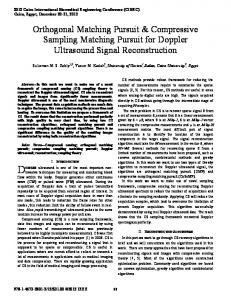
but also a list of other high-probability models Sˆ⋆ along with their posterior probabilities; the other six approaches considered return only a single model estimate. Thus, FBMP is able to give a more complete interpretation of the data in the face of ambiguity arising from correlation in A or from measurement noise. Fig. 3 shows average sparsity of solutions. We observe that, for this “compressible” signal and Gaussian regressor matrix, the coefficient estimates returned by FBMP are among the sparsest. In a second experiment, to illustrate the behavior of the greedy tree-search, we adopt a figure format used by George and McCulloch [45] to report MCMC results. To allow exhaustive evaluation of all candidate models, we set N = 26 and M = 7. Signals were constructed using the Gaussian mixture model of Section III with Q = 2, λ1 = 0.04, µ1 = 0, σ12 = 1, and with noise power adjusted to yield 10 dB SNR. For illustration, FBMP was provided the true hyperparameters and used without generalized
EM. Shown in Fig. VI is a rank-ordered list of the posterior probabilities p(s|y). To the right of the dashed line are the probabilities for the 59 models s selected by the search, while to the left of the dashed line are the probabilities for models not visited (truncated to show only the top 500, out of 226 − 59,
March 9, 2009
DRAFT
IEEE TRANSACTIONS ON SIGNAL PROCESSING
21
N = 26, M = 7, SNR = 10 dB, λ = 0.04, σ2 = 1, µ = 0, D 1
0
1
1
max
= 20
10
−1
10
−2
p(s|y)
10
−3
10
−4
10
−5
10
Top Unexplored Mixture Vectors
Top Explored Mixture Vectors
−6
10
Fig. 4.
Rank ordered mixture vector indices
Rank ordered posterior probabilities, on a logarithmic scale, of the models s visited by the search heuristic (right of
dashed vertical line) and the top 500 models not visited (left of dashed vertical line).
models). While the figure displays only one realization, it is typical of our numerical experience. The figure shows that, i) there exist multiple models with high probability, highlighting the inadequacy of reporting on the MAP model, and, ii) the low-complexity search heuristic is effective in visiting the high probability models. In a third experiment, an exhaustive evaluation similar to the previous one was repeated 204 times (see Table II for details), and each time both FBMP and the Larsson-Sel´en algorithm (LSA) [36] were used to compute estimates of x. The resulting average MSE performance is reported in Table II, along with ˆ denotes the estimate returned by ˆ mmse k22 , where x the average “distance to MMSE” (D2MMSE) kˆ x−x ˆ mmse denotes the exact MMSE estimate. It can be seen that FBMP the (FBMP or LSA) algorithm and x
clearly outperforms LSA both in terms of MSE and D2MMSE. In a fourth experiment, we carried out a “multiscale-CS” recovery of the popular “Mondrian” test image. Under the multiscale-CS framework, random Gaussian ensemble measurements were acquired from the 3 finest-scale Haar wavelet coefficients of the 128 × 128 image. In all, 4877 measurements were acquired from the 16384 unknowns, with different scales being undersampled by different factors. For comparison, recoveries were obtained using GPSR as well. The results of this experiment are shown in Fig. 5, with NMSEs and runtimes reported in the caption. The reported runtimes correspond to the time
March 9, 2009
DRAFT
IEEE TRANSACTIONS ON SIGNAL PROCESSING
22
Algorithm
MSE [dB]
D2MMSE [dB]
FBMP
−19.7
−24.1
LSA
−8.8
−9.1
TABLE II P ERFORMANCE FOR B ERNOULLI / IID -G AUSSIAN SIGNAL WITH N = 24, M = 8, Q = 2, λ1 = 0.04, µ1 = 0, σ12 = 1,
AND
SNR= 15 dB, AVERAGED OVER 204 TRIALS . S EE TEXT FOR DEFINITION OF D2MMSE.
(a) Original image
(b) FBMP recovery
(c) GPSR recovery
20
20
20
40
40
40
60
60
60
80
80
80
100
100
100
120
120 20
40
60
80
100
120
120 20
40
60
80
100
120
20
40
60
80
100
120
Fig. 5. Multiscale CS recovery. a) Original 128 × 128 image; b) FBMP recovery: NMSE = −16.80 dB, 8.85% of coefficients active, 38 minutes runtime; c) GPSR recovery: NMSE = −13.66 dB, 24.02% of coefficients active, 2.7 minutes runtime.
taken after the adjustable algorithmic parameters (e.g., τ for GPSR) were optimized. Relative to GPSR, the estimate returned by FBMP was more sparse and had lower NMSE, but took longer to generate. We note that these results are consistent with those from the other experiments. VII. D ISCUSSION A. Fast Algorithms: Related Works A Gaussian mixture model similar to that in Section III was likewise adopted by Larsson and Sel´en [36], who, for Q = 2, also constructed the MMSE estimate in the manner of (21) but with an S⋆ that contains exactly one model vector s for each Hamming weight 0 to N . They proposed to find these s via greedy deflation, i.e., starting with an all-active model configuration and recursively deactivating one component at a time. Thus, the D = 1 version of the BMP heuristic from Section IV-C recalls the heuristic of [36], but in reverse. Note, however, that the fast D = 1 BMP presented in Section IV-D has a complexity of only O(N M P ), in comparison to O(N 3 M 2 ) for the technique in [36]. Given the typically large values of N encountered in practice, the complexity of FBMP can be several orders of magnitude lower than
March 9, 2009
DRAFT
IEEE TRANSACTIONS ON SIGNAL PROCESSING
23
that of [36]. Complexity aside, Table II suggests that the greedy deflation approach of [36] is much less effective at finding the models vectors with high posterior probability, leading to estimates that, relative to FBMP, have higher MSE and are further from the exact MMSE estimate. For Q = 2, a Gaussian mixture model has been widely adopted for the Bayesian variable selection problem. (See, e.g., [1] for a survey and references.) The published approaches vary in prior specification, posterior calculation, and MCMC method (such as Gibbs sampler or Metropolis-Hastings). George and McCulloch [45] use a conjugate normal prior on x|s, σ 2 and a Gibbs sampler that requires O(N 2 ) operations to compute p(s′ |y) from p(s|y), where s′ and s differ in only one element. Smith and Kohn [32] use the point mass null (i.e., µ0 = σ02 = 0) and the simplifying Zellner-g prior to achieve a fast update requiring O(Ks2 ) operations, for Ks , ksk0 . Approximately M N iterations of the Gibbs sampler are suggested, yielding a total complexity of O(M N 2 Ks2 ). B. Bayesian Model Averaging The Bayesian framework provides a report on the confidence of estimates for both the model s and the coefficients x. In contrast, confidence labels are absent in most of the compressive sampling literature. ˆ⋆ for variable selection Exceptions are found in [16], [31], which use an (approximate) MAP estimate s ˆ⋆ being the true model. and report the Gaussian error covariance for the linear problem conditioned on s
As noted by Tibshirani [16], such a measure of posterior uncertainty has dubious value, because “a difficulty with this formula is that it gives an estimated variance of 0 for predictors with” [ˆ s⋆ ]n = 0. In ˆ⋆ is often not equal to the true s. Indeed, in order for s ˆ⋆ to fact, in our simulations, we observe that s
equal true s with high probability, for fixed sparsity ksk0 /N , the SNR grows unbounded with N [46]. In this light, we expect certain advantages for algorithms that consider the active signal coefficients as implicitly uncertain. As a caveat, we emphasize that our greedy FBMP search returns only Sˆ⋆ , an estimate of the dominant subset S⋆ , along with the values of ν(s, y) for s ∈ Sˆ⋆ . Thus, while the values ν(s, y) returned by FBMP can be used to compute exact ratios between the posterior probabilities of the model vectors in Sˆ⋆ , the true posteriors of these configurations (as approximated by (37) with Sˆ⋆ in place of S⋆ ) will only be accurate when Sˆ⋆ indeed contains S⋆ . In simulation, we observe that the proposed greedy FBMP search reliably discovers S⋆ when
March 9, 2009
λ1 N M
≤ −1/ log(λ1 ).
DRAFT
IEEE TRANSACTIONS ON SIGNAL PROCESSING
24
C. Empirical Bayes Empirical Bayes (EB) approaches have been used in related work to estimate hyperparameters from the data under signal models similar to the zero-mean binary prior given in Section III. George and Foster [47] adopted maximum marginal likelihood as in (40) for estimating parameters {λ1 , σ12 } en route to a MAP model selection using the Zellner g -prior. A forward greedy search for the EB sˆ⋆ was considered. For A = I , Johnstone and Silverman [48] used maximum marginal likelihood for λ1 and established the
asymptotic risk of adaptive thresholding rules. Larsson and Sel´en [36] likewise estimated hyperparameters from the data; for M ≥ N , ad hoc estimates were computed from the full-model least-squares estimate using higher-order moments. D. Informative Priors In our proposed approach, we have sought to incorporate physically meaningful prior knowledge when application-specific insight is available. Further, by use of the generalized-EM algorithm, we have provided a means for trade-off of complexity versus prior knowledge, i.e., ML estimates of hyperparameters may be iteratively estimated from the data. In contrast, the aim in statistical literature is to be agnostic by adopting noninformative priors or hyperpriors. VIII. C ONCLUSION In this paper, we proposed an algorithm for joint model selection and sparse coefficient estimation, which we call fast Bayesian matching pursuit (FBMP). We adopted a Bayesian approach in which a set of likely model configurations is reported, along with exact ratios of model posterior probabilities. These relative probabilities serve to reveal potential ambiguity among multiple candidate solutions that are ambiguous due to observation noise or correlation among columns in the regressor matrix. The ˆ, explicit management of uncertainty is essential for applications in which the estimated model vector, s ˆ , are not final products, but are instead statistics for use in making inference and estimated coefficients, x
from the noisy observations, y . The proposed search for high probability models and computation of their posteriors is fast in that the computational complexity is O(M N K), with M observations, N coefficients, and K nonzero coefficients. For a modest increase in complexity, the proposed generalized-EM refinement combines with FBMP to provide an empirical Bayes method for estimating hyperparameters from the data. Existing approaches using tree searches or MCMC methods require at least O(M N 2 K 2 ) computation. In forthcoming work we will report on a large-scale version of FBMP that reduces the memory required in recursively computing posterior probabilities, and we will give a bound on the probability that a subset March 9, 2009
DRAFT
IEEE TRANSACTIONS ON SIGNAL PROCESSING
25
of coefficients is absent from the MAP model estimate. R EFERENCES [1] M. Clyde and E. I. George, “Model uncertainty,” Statist. Sci., vol. 19, no. 1, pp. 81 – 94, 2004. [2] C. Volinsky, “Bayesian model averaging homepage,” http://www.research.att.com/˜volinsky/bma.html. [3] J. H¨ogbom, “Aperture synthesis with a non-regular distribution of interferometer baselines,” Astrophys. J. Suppl. Ser, vol. 15, pp. 417–426, 1974. [4] P. J. Huber, “Projection pursuit,” The Annals of Statistics, vol. 13, pp. 435–475, 1985. [5] Y. C. Pati, R. Rezaiifar, and P. S. Krishnaprasad., “Orthogonal matching pursuit: Recursive function approximation with applications to wavelet decomposition,” in Proc. 27th Ann. Asilomar Conf. Signals, Systems, and Computers, 1993. [6] D. Needell and J. A. Tropp, “CoSaMP: Iterative signal recovery from incomplete and inaccurate samples,” Harmon. Anal., 2008. doi:10.1016/j.acha.2008.07.002. [7] W. Dai and O. Milenkovic, “Subspace pursuit for compressive sensing: Closing the gap between performance and complexity,” Mar. 2008. preprint. [8] E. Cand`es, J. Romberg, and T. Tao, “Stable signal recovery from incomplete and inaccurate measurements,” Communications on Pure and Applied Mathematics, vol. 59, no. 8, pp. 1207–1223, 2006. [9] C. L. Lawson, Contributions to the theory of linear least maximum approximations. PhD thesis, UCLA, 1961. [10] H. Lee, D. Sullivan, and T. Huang, “Improvement of discrete band-limited signal extrapolation by iterative subspace modification,” in IEEE International Conference on Acoustics, Speech and Signal Processing, pp. 1569 – 1572, 1987. [11] I. F. Gorodnitsky and B. D. Rao, “Sparse signal reconstruction from limited data using FOCUSS: a re-weighted minimum norm algorithm,” IEEE Trans. Signal Process., vol. 45, pp. 600 – 616, Mar. 1997. [12] R. Chartrand and W. Yin, “Iteratively reweighted algorithms for compressive sensing,” in IEEE International Conference on Acoustics, Speech and Signal Processing, ICASSP 2008, (Las Vegas, NV), pp. 3869 – 3872, April 2008. [13] H. L. Taylor, S. C. Banks, and J. F. McCoy, “Deconvolution with the ℓ1 norm,” Geophysics, vol. 44, pp. 39–52, 1979. [14] A. E. Hoerl and R. W. Kennard, “Ridge regression: Biased estimation for nonorthogonal problems,” Technometrics, vol. 12, pp. 55–67, 1970. [15] S. S. Chen, D. L. Donoho, and M. A. Saunders, “Atomic decomposition by basis pursuit,” SIAM Journal on Scientific Computing, vol. 20, no. 1, pp. 33–61, 1998. [16] R. Tibshirani, “Regression shrinkage and selection via the lasso,” J. R. Statist. Soc. B, vol. 58, no. 1, pp. 267 – 288, 1996. [17] C. Bouman and K. Sauer, “A generalized Gaussian image model for edge-preserving MAP estimation,” IEEE Trans. Image Process., vol. 2, pp. 296–310, Mar. 1993. [18] A. H. Delaney and Y. Bresler, “A fast and accurate Fourier algorithm for iterative parallel-beam tomography,” IEEE Trans. Image Process., vol. 5, pp. 740–753, May 1996. [19] M. C ¸ etin and W. C. Karl, “Feature-enhanced synthetic aperture radar image formation based on nonquadratic regularization,” IEEE Trans. Image Process., vol. 10, pp. 623–631, Apr. 2001. [20] S. Levy and P. K. Fullagar, “Reconstruction of a sparse spike train from a portion of its spectrum and application to high-resolution deconvolution,” Geophysics, vol. 46, no. 9, pp. 1235–1243, 1981. [21] B. D. Rao and K. Kreutz-Delgado, “An affine scaling methodology for best basis selection,” IEEE Trans. Signal Processing, vol. 47, pp. 187–200, Jan. 1999.
March 9, 2009
DRAFT
IEEE TRANSACTIONS ON SIGNAL PROCESSING
26
[22] E. Cand`es, J. Romberg, and T. Tao, “Robust uncertainty principles: Exact signal reconstruction from highly incomplete frequency information,” IEEE Trans. Information Theory, vol. 52, pp. 489–509, Feb. 2006. [23] L. I. Rudin, S. Osher, and E. Fatemi, “Nonlinear total variation based noise removal algorithms,” Physica D, vol. 60, pp. 259 – 268, 1992. [24] D. L. Donoho, M. Elad, and V. N. Temlyakov, “Stable recovery of sparse overcomplete representations in the presence of noise,” IEEE Trans. Information Theory, vol. 52, pp. 6–18, Jan. 2006. [25] J. A. Tropp, “Just relax: Convex programming methods for identifying sparse signal,” IEEE Trans. Info. Theory, vol. 51, pp. 1030–1051, Mar. 2006. [26] T. Tao, “Open question: deterministic UUP matrices,” July 2007. http://terrytao.wordpress.com/2007/07/02/open-questiondeterministic-uup-matrices/. [27] Y. T. Lo, “A mathematical theory of antenna arrays with randomly spaced elements,” IEEE Trans. Antennas and Propagation, vol. 12, pp. 257–268, 1964. [28] G. J. Marseille, R. de Beer, M. Fuderer, A. F. Mehlkopf, and D. van Ormondt, “Nonuniform phase-encode distributions for MRI scan time reduction,” J. Magn. Reson., vol. 111, pp. 70–75, 1996. [29] M. E. Tipping, “Sparse Bayesian learning and the relevance vector machine,” J. Machine Learning Res., vol. 1, pp. 211–244, 2001. (software available at http://www.miketipping.com/index.php?page=rvm). [30] D. Wipf and B. Rao, “Sparse Bayesian learning for basis selectionn,” IEEE Trans. Signal Process., vol. 52, pp. 2153 – 2164, Aug. 2004. [31] S. Ji and L. Carin, “Bayesian compressive sensing and projection optimization,” in Proc. 24th Int. Conf. Machine Learning (ICML), pp. 377 – 384, 2007. (software available at http://www.ece.duke.edu/˜shji/BCS.html). [32] M. Smith and R. Kohn, “Nonparametric regression using Bayesian variable selection,” J. Econometrics, vol. 75, pp. 317 – 343, 1996. [33] C. Andrieu, A. Doucet, and C. P. Robert, “Computational advances for and from Bayesian analysis,” Statist. Sci., vol. 19, no. 1, pp. 118 – 127, 2004. [34] P. J. Wolfe, S. J. Godsill, and W.-J. Ng, “Bayesian variable selection and regularization for time-frequency surface estimation,” J. R. Statist. Soc. B, vol. 66, pp. 575–589. [35] M. Elad and I. Yavneh, “A weighted average of sparse representations is better than the sparsest one alone,” 2008. preprint. [36] E. Larsson and Y. Sel´en, “Linear regression with a sparse parameter vector,” IEEE Trans. Signal Process., vol. 55, pp. 451 – 460, Feb. 2007. [37] S. Som, L. C. Potter, R. Ahmad, D. S. Vikram, and P. Kuppusamy, “EPR oximetry in three spatial dimensions using sparse spin distribution,” Journal of Magnetic Resonance, vol. 193, Aug. 2008. [38] H. V. Poor, An Introduction to Signal Detection and Estimation. Springer, 2 ed., 1994. [39] A. P. Dempster, N. M. Laird, and D. B. Rubin, “Maximum likelihood from incomplete data via the EM algorithm,” J. R. Statist. Soc. B, vol. 39, no. 1, pp. 1–38, 1977. [40] R. Neal and G. Hinton, “A view of the EM algorithm that justifies incremental, sparse, and other variants,” in Learning in Graphical Models (M. I. Jordan, ed.), pp. 355–368, MIT Press, 1999. [41] J. Tropp and A. Gilbert, “Signal recovery from random measurements via orthogonal matching pursuit,” IEEE Trans. Information Theory, vol. 53, pp. 4655–4666, Dec. 2007. (software available at http://sparselab.stanford.edu/). [42] D. L. Donoho, Y. Tsaig, I. Drori, and J.-C. Starck, “Sparse solution of underdetermined linear equations by stagewise
March 9, 2009
DRAFT
IEEE TRANSACTIONS ON SIGNAL PROCESSING
27
orthogonal matching pursuit,” Tech. Rep. 2006-02, Dept. of Statistics, Stanford University, Stanford, CA, 2006. (software available at http://sparselab.stanford.edu/). [43] M. A. T. Figueiredo, R. D. Nowak, and S. J. Wright, “Gradient projection for sparse reconstruction: Application to compressed sensing and other inverse problems,” IEEE Journal of Selected Topics in Signal Processing, vol. 1, no. 4, pp. 586–597, 2007. (software available at http://www.lx.it.pt/˜mtf/GPSR/). [44] C. M. Bishop and M. E. Tipping, “Variational relevance vector machines,” in Proceedings of the 16th Conf. on Uncertainty in Artificial Intelligence (C. Boutilier and M. Goldszmidt, eds.), pp. 46–53, Morgan Kaufmann, 1999. (software available at http://people.ee.duke.edu/˜lihan/cs/). [45] E. I. George and R. E. McCulloch, “Approaches for Bayesian variable selection,” Statistica Sinica, vol. 7, pp. 339 – 373, 1997. [46] G. Reeves, “Sparse signal sampling using noisy linear projections,” Master’s thesis, EECS Department, University of California, Berkeley, 2008. [47] E. I. George and D. P. Foster, “Calibration and empirical Bayes variable selection,” Biometrika, vol. 87, no. 4, pp. 731 – 747, 2000. [48] I. M. Johnstone and B. W. Silverman, “Needles and straw in haystacks: Empirical Bayes estimates of possibly sparse sequences,” Ann. Stat., vol. 32, no. 4, pp. 1594 – 1649, 2004.
A PPENDIX A M EAN
AND
VARIANCE
OF
ν(s, y)
In this appendix, we derive the mean and variance of ν(s, y). According to our priors, if s is the model vector from which y is generated, then y = Ax+w for x|s ∼ CN (µ(s), R(s)) and w ∼ CN (0, σ 2 I M ). ¯
This implies that y − Aµ(s) ¯ s ∼ CN (0, Φ(s)), so that ¡
¢H
y − Aµ(s)
¡
¢
Φ(s)−1 y − Aµ(s)
∼ χ2M ,
(68)
i.e., a chi-squared random variable with M degrees of freedom. Say that As denotes the matrix constructed from the active columns of A. Then, if σq2 = σ12 for all q 6= 0 (as in all the examples given in Section III) and if As is orthonormal, ¡
ln det(Φ(s)) = ln (σ12 + σ 2 )ksk0 σ 2(M −ksk0 ) 2
= ksk0 ln( σσ12 + 1) + M ln σ 2 ,
¢
(69) (70)
where ksk0 ∼ Binomial(N, 1 − λ0 ). The orthonormal assumption on As is reasonable because the columns of A were assumed unit-norm in Section III and, for the class of problems that guarantee good sparse estimates, any collection of ksk0 columns from A will be approximately orthogonal. (Recall the restricted isometry property [8].) Finally, if we assume that λq = λ1 for all q 6= 0 (as in all the examples
March 9, 2009
DRAFT
IEEE TRANSACTIONS ON SIGNAL PROCESSING
28
given in Section III), then N −1 X
ln λsn = ksk0 ln λ1 + (N − ksk0 ) ln λ0
(71)
n=0
= N ln λ0 − ksk0 ln λλ01 .
(72)
Using the facts that the mean and variance of a χ2M random variable are M and 2M , respectively, and the mean and variance of ksk0 are N (1 − λ0 ) and N (1 − λ0 )λ0 , respectively, we obtain (25). A PPENDIX B D ERIVATION
OF
(31)
In this appendix, we establish (31) using (27)-(30). Using the fact that Φ(s)−1 an = cn , we find ¡
¢H
¡
y − Aµ(s′ ) ¡
= y − Aµ(s) − an µq′ ,q ¡
¢H ¡
× y − Aµ(s) − an µq′ ,q ¡
¢H
= y − Aµ(s) ¯
¢
Φ(s′ )−1 y − Aµ(s′ )
¡
¡
Φ(s)−1 − βn,q′ cn cH n
¢
(73) ¢
Φ(s)−1 y − Aµ(s) ¢¯
¯2 − βn,q′ ¯cH n y − Aµ(s) ©
¢
¡
¢ª
−1 − 2 Re µ∗q′ ,q aH y − Aµ(s) n Φ(s)
©
¡
¢ª
H + 2 Re µ∗q′ ,q aH n cn βn,q ′ cn y − Aµ(s)
H 2 −1 2 + |µq′ ,q |2 aH n Φ(s) an − |µq ′ ,q | βn,q ′ (cn an )
¡
¢H
= y − Aµ(s) ¯
¡
¡
¢
Φ(s)−1 y − Aµ(s) ¢¯
¯2 − βn,q′ ¯cH n y − Aµ(s) ©
(74)
¡
¢¡
H − 2 Re µ∗q′ ,q cH n y − Aµ(s) 1 − βn,q ′ an cn
¡
¢
H + |µq′ ,q |2 cH n an 1 − βn,q ′ an cn .
¢ª
(75)
In the case that σq2′ ,q = 0, we have βn,q′ = 0, and so ¡
¢H
y − Aµ(s′ ) ¡
¢H
= y − Aµ(s) ©
¡
¢
Φ(s′ )−1 y − Aµ(s′ ) ¡
¡
¢ª
− 2 Re µ∗q′ ,q cH n y − Aµ(s)
March 9, 2009
¢
Φ(s)−1 y − Aµ(s)
+ |µq′ ,q |2 cH n an .
(76)
DRAFT
IEEE TRANSACTIONS ON SIGNAL PROCESSING
29
−2 In the case that σq2′ ,q 6= 0, we have 1 − βn,q′ aH n cn = −βn,q ′ σq ′ ,q , so that
¡
¢H
y − Aµ(s′ ) ¡
¡
¢
Φ(s′ )−1 y − Aµ(s′ ) ¢H
= y − Aµ(s) · ¯
¡
¡
¢¯
¯2 − βn,q′ ¯cH n y − Aµ(s) ©
¡
¢ µ∗q′ ,q ª
− 2 Re cH n y − Aµ(s) ¡
¢H
= y − Aµ(s) ¯ ¯
¡
¡
σq2′ ,q
¡
¢
¢H
¯ ¯
¡
¡
¢
Together, (76) and (79) yield (80).
¢H
=
¸
(77)
¢
µq′ ,q ¯¯2 ¯ σq2′ ,q
(78) ¢
Φ(s)−1 y − Aµ(s)
− βn,q′ ¯cH n y − Aµ(s) +
y − Aµ(s′ )
|µq′ ,q |2 σq2′ ,q
i |µq′ ,q |2 h 2 H 1 + σ c a ′ n q ,q n σq4′ ,q
= y − Aµ(s)
¡
+ cH n an
Φ(s)−1 y − Aµ(s)
− βn,q′ ¯cH n y − Aµ(s) +
+ βn,q′
¢
Φ(s)−1 y − Aµ(s)
¡
µq′ ,q ¯¯2 |µq′ ,q |2 . ¯ + σq2′ ,q σq2′ ,q
(79)
¢
Φ(s′ )−1 y − Aµ(s′ )
¡ ¢H ¡ ¢ −1 y − Aµ(s) y − Aµ(s) Φ(s) ¯ H¡ ¯2 ¢ 2 ′ ¯c ′ ,q /σ ′ ¯ − β y − Aµ(s) + µ n,q q n q ,q + |µq′ ,q |2 /σq2′ ,q ¡ ¢ ¡ ¢H y − Aµ(s) Φ(s)−1 y − Aµ(s) © ¡ ¢ª − 2 Re µ∗q′ ,q cH n y − Aµ(s) + |µq′ ,q |2 cH n an
σq2′ ,q 6= 0 .
(80)
σq2′ ,q = 0.
Equation (27) then implies that
¡
ln det(Φ(s′ )) = ln det Φ(s) + σq2′ ,q an aH n = ln
h¡
¢
¢
(81) ¡
¢i
−1 1 + σq2′ ,q aH n Φ(s) an det Φ(s)
= ln det(Φ(s)) − ln(βn,q′ /σq2′ ,q ) ln p(s′ ) = ln p(s) + ln(λq′ /λq ),
(82) (83)
which, in conjunction with (18) and (80), yield (31).
March 9, 2009
DRAFT