Fast Parallel Randomized Algorithm for Nonnegative Matrix

Fast Parallel Randomized Algorithm for Nonnegative Matrix Factorization with KL Divergence for Large Sparse Datasets arXiv:1604.04026v1 [math.OC] 14 Apr 2016

Duy Khuong Nguyen, Tu Bao Ho Abstract—Nonnegative Matrix Factorization (NMF) with Kullback-Leibler Divergence (NMF-KL) is one of the most significant NMF problems and equivalent to Probabilistic Latent Semantic Indexing (PLSI), which has been successfully applied in many applications. For sparse count data, a Poisson distribution and KL divergence provide sparse models and sparse representation, which describe the random variation better than a normal distribution and Frobenius norm. Specially, sparse models provide more concise understanding of the appearance of attributes over latent components, while sparse representation provides concise interpretability of the contribution of latent components over instances. However, minimizing NMF with KL divergence is much more difficult than minimizing NMF with Frobenius norm; and sparse models, sparse representation and fast algorithms for large sparse datasets are still challenges for NMF with KL divergence. In this paper, we propose a fast parallel randomized coordinate descent algorithm having fast convergence for large sparse datasets to archive sparse models and sparse representation. The proposed algorithm’s experimental results overperform the current studies’ ones in this problem. Index Terms—Nonnegative Matrix Factorization, KullbackLeibler Divergence, Sparse Models, and Sparse Representation

I. I NTRODUCTION The development of technology has been generating big datasets of count sparse data such as documents and social network data, which requires fast effective algorithms to manage this huge amount of information. One of these tools is nonnegative matrix factorization (NMF) with KL divergence, which is proved to be equivalent with Latent Semantic Indexing (PLSI) [2]. NMF is a powerful linear technique to reduce dimension and to extract latent topics, which can be readily interpreted to explain phenomenon in science [3], [6], [12]. NMF makes postprocessing algorithms such as classification and information retrieval faster and more effective. In addition, latent factors extracted by NMF can be more concisely interpreted than other linear methods such as PCA and ICA [12]. In addition, NMF is flexible with numerous divergences to adapt a large number of real applications [14], [15]. For sparse count data, NMF with KL divergence and a Poisson distribution may provide sparse models and sparse representation describing better the random variation rather than NMF with Frobenius norm and a normal distribution [13]. For example, the appearance of words over latent topics and of topics over documents should be sparse. However, achieving sparse models and sparse representation is still a

major challenge because minimizing NMF with KL divergence is much more difficult than NMF with Frobenius norm [5]. In the NMF-KL problem, a given nonnegative data matrix V ∈ Rn×m must be factorized into a product of two nonneg+ ative matrices, namely a latent component matrix W ∈ Rr×n + and a representation matrix F ∈ Rr×m , where n is the + dimension of a data instance, m is the number of data instances, and r is the number of latent components or latent factors. The quality of this factorization is controlled by the objective function with KL divergence as follows: D(V kW T F ) =

m n X X

(Vij log

i=1 j=1

Vij −Vij +(W T F )ij ) (1) (W T F )ij

In the general form of L1 and L2 regularization variants, the objective function is written as follows: D(V kW T F ) +

α1 α2 kW k22 + kF k22 + β1 kW k1 + β2 kF k1 (2) 2 2

NMF with KL divergence has been widely applied in many applications for dense datasets. For example, spatially localized, parts-based subspace representation of visual patterns is learned by local non-negative matrix factorization with a localization constraint (LNMF) [8]. In another study, multiple hidden sound objects from a single channel auditory scene in the magnitude spectrum domain can be extracted by NMF with KL divergence [11]. In addition, two speakers in a single channel recording can be separated by NMF with KL divergence and L1 regularization on F [10]. However, the existing algorithms for NMF with KL divergence (NMF-KL) are extremely time-consuming for large count sparse datasets. Originally, Lee and Seung, 2001 [7] proposed the first multiple update iterative algorithm based on gradient methods for NMF-KL. Nevertheless, this technique is simple and ineffective because it requires a large number of iterations, and it ignores negative effects of nonnegative constraints. In addition, gradient methods have slow convergence for complicated logarithmic functions like KL divergence. Subsequently, Cho-Jui & Inderjit, 2011 [4] proposed a cycle coordinate descent algorithm having low complexity of one variable update. However, this method contains several limitations: first, it computes and stores the dense product matrix W T F although V is sparse; second, the update of W T F for the change of each cell in W and F is considerably complicated, which leads to practical difficulties in parallel

and distributed computation; finally, the sparsity of data is not considered, while large datasets are often highly sparse. In comparison with NMF with Frobenius norm, NMF with KL divergence is much more complicated because updating variables will influence derivatives of other variables; this computation is extremely expensive. Hence, it is difficult to employ fast algorithms having multiple variable updates, which limits the number of effective methods. In this paper, we propose a new advanced version of coordinate descent methods with significant modifications for large sparse datasets. Regarding the contributions of this paper, we: • Propose a fast sparse randomized coordinate descent algorithm using limited internal memory for nonnegative matrix factorization for huge sparse datasets, the full matrix of which can not stored in the internal memory. In this optimization algorithm, variables are randomly selected with uniform sampling to balance the order priority of variables. Moreover, the proposed algorithm effectively utilizes the sparsity of data, models and representation matrices to improve its performance. Hence, the proposed algorithm can be considered an advanced version of cycle coordinate descent for large sparse datasets proposed in [4]. • Design parallel algorithms for combinational variants of L1 and L2 regularizations. • Indicate that the proposed algorithm using limited memory can fast attain sparse models, sparse representation, and fast convergence by evaluational experiments, which is a significant milestone in this research problem for large sparse datasets. The rest of the paper is organized as follows. Section II presents the proposed algorithms. The theoretical analysis of convergence and complexity is discussed in Section III. Section IV shows the experimental results, and Section V summarizes the main contributions of this pape and discussion.

Specially, a number of optimization problems D(Vi kW T Fi ) or D(VjT kF T Wj ) in Algorithm 1 with the form D(vkAx) can be independently and simultaneously solved by Algorithm 2. In this paper, we concern combinational variants of NMF KL divergence with L1 and L2 regularizations in the general formula, Function 4: Algorithm 1: Iterative multiplicative update

1 2 3 4 5

6 7

8 9 10

11 12

13 14 15

16

Input: V ∈ Rn×m , r, and α1 , α2 , β1 , β2 ≥ 0 + r×m Output: W ∈ Rn×r . + , F ∈ R+ begin r×n Randomize W ∈ R+ ; r×m Randomize F ∈ R+ ; while convergence condition is not satisfied do ids = a randomized ordered set of values {1, 2, ..., r}; sumW = W 1n ; /*Optimizing the objective function by F when fixing W */; for j = 1 to m do /*Call Algorithm 2 in parallel*/; Fjk+1 = Algorithm 2 (Vj , W T , sumW , Fjk , α2 , β2 , ids) sumF = F 1m ; /*Optimizing the objective function by W when fixing F */; for i = 1 to n do /*Call Algorithm 2 in parallel*/; Wik+1 = Algorithm 2 (ViT F T , sumW , Wik , α2 , β2 , ids); return (W k+1 )T , F k+1 ;

f (x) = D(vkAx) =

II. P ROPOSED A LGORITHM

D(V kW F ) =

i=1

T

D(Vi kW Fi ) =

n X

D(VjT kF T Wj )

(3)

α vi −vi +[Ax]i )+ kxk22 +β|x|1 [Ax]i 2 (4)

r where v ∈ Rn+ , A ∈ Rn×r + , x ∈ R+ Because the vector v is given, minimizing Function 4 is equivalent to minimizing Function 5:

f (x) = D(vkAx) =

n X

(−vi log [Ax]i + [Ax]i ) +

i=1

α kxk22 + β|x|1 2 (5)

From Equation 5, the first and second derivative of the variable xk are computed by Formula 6:

⇒ m X

(vi log

i=1

In this section, we propose a fast sparse randomized coordinate descent parallel algorithm for nonnegative sparse matrix factorization on Kullback-Leibler divergence. We employ a multiple iterative update algorithm like EM algorithm, see Algorithm 1, because D(V kW T F ) is a non-convex function although it is a convex function when fixing one of two matrices W and F . This algorithm contain a while loop containing two main steps: the first one is to optimize the objective function by F when fixing W ; and the another one is to optimize the objective function by W when fixing F . Furthermore, in this algorithm, we need to minimize Function 3, the decomposed elements of which can be independently optimized in Algorithm 1: T

n X

   ∇fk   ∇2 fkk

=−

n P i=1

=

n P

i=1

Aik vi [Ax] + i

n P i=1

Aik + αxk + β (6)

Aik 2 vi ( [Ax] ) +α i

j=1

Based on Formula 6, we have several significant remarks:

One update of xk changes all elements of Ax, which are under the denominators of fractions. Hence, it is difficult to employ fast algorithms having simultaneous updates of multiple variables because it will require heavy computation. Hence, we employ coordinate descent methods to reduce the complexity of each update, and to avoid negative effects of nonnegative constraints. • One update of xk has complexity of maintaining ∇fk 2 and Pn ∇ fkk as O(k + nnz(v) + nnz(v)) = k + nnz(v) if i=1 Aik is computed in advance. Specially, it employs O(k + nnz(v)) of multiple and addition operators, and exactly O(nnz(v)) of divide operators; where nnz(v) is the number of non-zero elements in the vector v. Hence, for sparse datasets, the number of operators can be negligible. • The used internal memory of Algorithm 1 and Algorithm 2 is O(nnz(V ) + size(W ) + size(F )) = nnz(V ) + (n + m)r, where nnz(V ) is the number of non-zero elements in the given matrix V , which is much smaller than O(mn + (n + m)r) for the existing algorithms [4], [7]. Hence, Algorithm 2 employs a coordinate descent algorithm based on projected Newton methods with quadratic approximation in Algorithm 2 is to optimize Function 5. Specially, because Function 5 is convex, a coordinate descent algorithm based on projected Newton method [9], [9] with quadratic approximation is employed to iteratively update with the nonnegative lower bound as follows:

Algorithm 2: Randomized coordinate descent algorithm for sparse datasets

•

xk = max(0, xk −

∇fk ) ∇2 fkk

Considering the limited internal memory and the sparsity of x, we maintain W T Fj via computing Ax instead of storing the dense matrix W T F for the following reasons: • The internal memory requirement will significantly decrease, so the proposed algorithm can stably run on limited internal memory machines. • The complexity of computing Ax is always smaller than the complexity of computing and maintaining ∇fk and ∇2 fkk , so it does not cause the computation more complicated. • The updating Ax = Ax + 4xAk as the adding with a scale of two vectors utilizes the speed of CPU cache because of accessing consecutive memory cells. • The recomputing helps remove the complexity of maintaining the dense product matrix W T F as in [4], [7], which is certainly considerable because this maintenance accesses memory cells far together and does not utilize CPU cache. In summary, in comparison with the original coordinate algorithm [4] for NMK-KL, the proposed algorithm involve significant improvements as follows: • Randomize the order of variables to optimize the objective function in Algorithm 2. Hence, the proposed algorithm can balance the order priority of variables,

Input: v ∈ Rn , A ∈ Rn×k , sumA, x ∈ Rk , α ≥ 0, β ≥ 0, and variable order ids Output: x is updated by n P x ≈ argmin −vi log([Ax]i + ) + [Ax]i + 1 2 3 4

5 6 7 8 9 10 11

x0 i=1 α 2 2 kxk2 + βkxk1 .

begin Compute Ax ∈ Rn ; for k in order ids do Compute ∇fk and ∇2 fkk based on α, β, v, x, Ax, sumA and sparsity of v based on Formula 6; while (∇fk < −) or (|∇fk | >  and xk > ) do k ) − xk ; 4x = max(0, xk − ∇∇f 2f kk Update Ax via Ax = Ax + 4xAk ; xs = xk ; xk = xk + 4x; if (4x < x xs) then break; Update ∇fk and ∇2 fkk based on α, β, v, x, sumA and sparsity of v based on Formula 6;

12

return x;

13

•

• • •

Remove duplicated computation of maintaining derivatives ∇fk and ∇2 fkk by computing common elements sumW = W 1n and sumF = F 1m in advance, which led to that the complexity of computing ∇fk and ∇2 fkk only depends on the sparsity of data, Effectively utilize the sparsity of W and F to reduce the running time of computing Ax, Effectively utilize CPU cache to improve the performance of maintaining Ax = Ax + 4xAk , Recompute Ax but remove the maintenance of the dense matrix product W T F . Hence, the proposed algorithm stably run on the limited internal memory systems with the required memory size O(nnz(V )+size(W )+size(F )) = nnz(V )+(m+n)r, which is much smaller than O(mn+ (n + m)r) for the existing algorithms [4], [7]. III. T HEORETICAL A NALYSIS

In this section, we analyze the convergence and complexity of Algorithm 1 and Algorithm 2. In comparison with the previous algorithm of Hsieh & Dhillon, 2011 [4], the proposed algorithm has significant modifications for large sparse datasets by means of adding the order randomization of indexes and utilizing the sparsity of data V , model W , and representation F . These modifications does not affect on the convergence guarantee of algorithm. Hence, based on Theorem 1 in Hsieh & Dhillon, 2011 [4],

Algorithm 2 converges to the global minimum of f (x). Furthermore, based on Theorem 3 in Hsieh & Dhillon, 2011 [4], Algorithm 1 using Algorithm 2 will converge to a stationary point. In practice, we set x = 0.1 in Algorithm 2, which is more precise than x = 0.5 in Hsieh & Dhillon, 2011 [4]. Concerning the complexity of Algorithm 2, based on the remarks in Section II, we have Theorem 1. Furthermore, because KL divergence is a convex function over one variable and the nonnegative domain, and project Newton methods with quadratic approximation for convex functions have superlinear rate of convergence [1], [9], the average number of iterations t¯ is small. Theorem 1. The complexity of Algorithm 2 is O(nnnz(r) + t¯r(r + n + nnz(n))), where nnz(r) is the number of non-zero elements in x, nnz(n) is the number of non-zero elements in v, and t¯ is the average number of iterations. Then, the complexity of a while iteration in Algorithm 1 is O(t¯(mnr + (m + n)r2 )) Proof: Consider the major computation in Algorithm 2, based on Formula 6, we have: • The complexity of computing Ax in Line 2 is O(nnnz(r)), 2 • The complexity of computing ∇fk and ∇ fkk in Line 4 is O(r + nnz(n)) because Ax and sumA are computed in advance, 2 • The complexity of updating ∇fk and ∇ fkk in Line 12 is O(r + n + nnz(n)) because only one dimension of vector x is changed. Hence, the complexity of Algorithm 2 is O(nnnz(r)+t¯r(r+ n + nnz(n))). In addition, the complexity of computing sumW and sumF is O((m + n)r). Hence, the complexity of a while iteration in Algorithm 1 is O((m + n)r + mnnnz(r) + t¯mr(r + n + nnz(n))) ≈ (m + n)r + t¯(mnr + (m + n)r2 ) ≈ t¯(mnr + (m + n)r2 ) Therefore, we have Theorem 1 For large sparse datasets, m, n  r ⇒ O(t¯(mnr + (m + n)r2 )) ≈ t¯(mnr). This complexity is raised by the operators Ax = Ax + 4xAk in Algorithm 2. To reduce the running time of these operators, Ak must be stored in an array to utilize CPU cache memory by accessing continuous memory cells of Ax and Ak . IV. E XPERIMENTAL E VALUATION In this section, we investigate the effectiveness of the proposed algorithm via convergence and sparsity. Specially, we compare the proposed algorithm Sparse Randomized Coordinate Descent (SRCD) with state-of-the-art algorithms as follows: • Multiplicative Update (MU) [7]: This algorithm is the original method for NMF with KL divergence. • Cycle Coordinate Descent (CCD) [4]: This algorithm has the current fastest convergence because it has very low complexity of each update for one variable. Datasets: To investigate the effectiveness of the algorithms compared, the 4 sparse datasets used are shown in Table I.

TABLE I: Summary of datasets Dataset (V ) Digits Reuters21578 TDT2 RCV1 4Class

n

m

nnz(V )

Sparsity (%)

784 8, 293 9, 394 9, 625

60, 000 18, 933 36, 771 29, 992

8, 994, 156 389, 455 1, 224, 135 730, 879

80.8798 99.7520 99.6456 99.7468

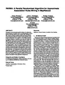
The dataset Digit is downloaded from 1 , and the other tf-idf datasets Reuters21578, TDT2, and RCV1 4Class are downloaded from 2 . Environment settings: We develop the proposed algorithm SRCD in Matlab with embedded code C++ to compare them with other algorithms. We set system parameters to use only 1 CPU for Matlab and the IO time is excluded in the machine Mac Pro 8-Core Intel Xeon E5 3 GHz 32GB. In addition, the initial matrices W 0 and F 0 are set to the same values. The source code will be published on our homepage 3 . A. Convergence In this section, we investigate the convergence of the objective value D(V ||W T F ) versus running time by running all the compared algorithms on the four datasets with two numbers of latent factors r = 10 and r = 20. The experimental results are depicted in Figure 1 and Figure 2. From these figures, we realize two significant observations as follows: • The proposed algorithm (SRCD) has much faster convergence than the algorithms CCD and MU, • The sparser the datasets are, the greater the distinction between the convergence of the algorithm SRCD and the other algorithms CCD and MU is. Specially, for Digits with 81% sparsity, the algorithm SRCD’s convergence is lightly faster than the convergence of the algorithms CCD and MU. However, for three more sparse datasets Reuters21578, TDT2, and RCV1 4Class with above 99% sparsity, the distance between these convergence speeds is readily apparent. B. Sparsity of factor matrices Concerning the sparsity of factor matrices W and F , the algorithms CCD and MU does not utilize the sparsity of factor matrices. Hence, these algorithms add a small number into these factor matrices to obtain convenience in processing special numerical cases. Hence, the sparsity of factor matrices W and F for the algorithms CCD and MU both are 0%. Although this processing may not affect other post-processing tasks such as classification and information retrieval, it will reduce the performance of these algorithms. The sparsity of (W, F ) of the proposed algorithm’s results is showed in Table II. These results clearly indicate that the sparse model W and the sparse representation F are attained. The results also explain why the proposed algorithm runs very fast on the 1 http://yann.lecun.com/exdb/mnist/ 2 http://www.cad.zju.edu.cn/home/dengcai/Data/TextData.html 3 http://khuongnd.appspot.com/

TABLE II: Sparsity (%) of (W, F ) for the algorithm SRCD’s results SRCD

CCD

MU

Digits with r = 10

TDT2 with r = 10

r = 10 r = 20

Digits

Reuters21578

TDT2

RCV1 4Class

(74.3, 49.2) (87.8, 49.7)

(75.6, 71.6) (84.2, 80.4)

(68.5, 71.3) (78.6, 81.1)

(81.2, 74.0) (88.4, 83.0)

107.4 D(V kW F )

109.4

TABLE III: Used internal memory (GB) for r = 10

107.2

109.2

Datasets

107 106.8

109 101 102 Reuters21578 with r = 10

103

101 102 103 104 RCV1 4Class with r = 10

CCD

SRCD

1.89 5.88 11.51 9.73

0.85 2.46 5.29 4.43

1.76 0.17 0.30 0.23

106

107 106.8

sparse datasets Reuters21578, TDT2 and RCV1 4Class, when it can obtain highly sparse models and sparse representation in these highly sparse datasets.

D(V kW T F )

105.8

106.6 105.6

106.4

C. Used internal memory 105.4

106.2 101

102 seconds

103

101

102 103 seconds

104

Fig. 1: Objective value D(V kW T F ) versus running time with r = 10

SRCD

CCD

Digits with r = 20

MU

1 D(V kW F )

D. Running on large datasets 107.4

105.6

This section investigates running the proposed algorithm on large datasets with different settings. Figure 3 shows the running time of Algorithm SRCD for 100 iterations with different number of latent component using 1 thread. Clearly, the running time linearly increases, which fits the theoretical analyses about fast convergence and linear complexity for large sparse datasets in Section III. Furthermore, concerning the parallel algorithm, the running time of Algorithm SRCD for 100 iterations significantly decreases when the number of used threads increases in Figure 4. In addition, the running time is acceptable for large applications. Hence, these results indicate that the proposed algorithm SRCD is feasible for large scale applications.

105.4

V. C ONCLUSION AND D ISCUSSION

107.2

109.2 107

109

106.8

108.8

106.6

101 102 103 Reuters21578 with r = 20 107

101

102 103 104 RCV1 4Class with r = 20

106

106.8

105.8

6.6

10

106.4 106.2 101

102 seconds

103

Table III shows the internal memory used by algorithms. From the table, we have two significant observations: • For the dense dataset Digits, the proposed algorithm SRCD uses more internal memory than the the algorithm CCD because a considerable amount of memory is used for the indexing of matrices. • For the sparse datasets Reuters21578, TDT2, and RCV1 4Class, the internal memory for SRCD is remarkably smaller than the internal one for MU and CCD. These results indicate that we can conduct the proposed algorithm for huge sparse datasets with a limited internal memory machine is stable.

TDT2 with r = 20

109.4

D(V kW T F )

Digits Reuters21578 TDT2 RCV1 4Class

MU

104

101

102

103 seconds

104

Fig. 2: Objective value D(V kW T F ) versus running time with r = 20

1

In this paper, we propose a fast parallel randomized coordinate descent algorithm for NMF with KL divergence for large sparse datasets. The proposed algorithm attains fast convergence by means of removing duplicated computation, exploiting sparse properties of data, model and representation matrices, and utilizing the fast accessing speed of CPU cache. In addition, our method can stably run systems within limited

Digits

Reuters21578

TDT2

RCV1 4Class

600

Running time (s)

500

400

300

200

100 10

20

30 r

40

50

Fig. 3: Running time of 100 iterations with different number of latent component using 1 thread Digits

Reuters21578

TDT2

RCV1 4Class

600

Running time (s)

500

1

400 300 200 100

1

2

3

4 5 Number of threads

6

7

8

Fig. 4: Running time of 100 iterations with r = 50 and using different number of threads

internal memory by reducing internal memory requirements. Finally, the experimental results indicate that highly sparse models and sparse representation can be attained for large sparse datasets, a significant1 milestone in researching this problem. In future research, we will generalize this algorithm for nonnegative tensor factorization. ACKNOWLEDGEMENTS This work is partially sponsored by Asian Office of Aerospace R&D under agreement number FA2386-15-1-4006, by funded by Vietnam National University at Ho Chi Minh City under the grant number B2015-42-02m, and by 911 Scholarship from Vietnam Ministry of Education and Training. R EFERENCES [1] D. P. Bertsekas. Projected newton methods for optimization problems with simple constraints. SIAM Journal on control and Optimization, 20(2):221–246, 1982.

[2] C. Ding, T. Li, and W. Peng. Nonnegative matrix factorization and probabilistic latent semantic indexing: Equivalence chi-square statistic, and a hybrid method. In Proceedings of the national conference on artificial intelligence, volume 21, page 342. Menlo Park, CA; Cambridge, MA; London; AAAI Press; MIT Press; 1999, 2006. [3] N. Gillis. The why and how of nonnegative matrix factorization. Regularization, Optimization, Kernels, and Support Vector Machines, 12:257, 2014. [4] C.-J. Hsieh and I. S. Dhillon. Fast coordinate descent methods with variable selection for non-negative matrix factorization. In Proceedings of the 17th ACM SIGKDD international conference on Knowledge discovery and data mining, pages 1064–1072. ACM, 2011. [5] D. Kuang, J. Choo, and H. Park. Nonnegative matrix factorization for interactive topic modeling and document clustering. In Partitional Clustering Algorithms, pages 215–243. Springer, 2015. [6] D. Lee, H. Seung, et al. Learning the parts of objects by non-negative matrix factorization. Nature, 401(6755):788–791, 1999. [7] D. D. Lee and H. S. Seung. Algorithms for non-negative matrix factorization. In Advances in neural information processing systems, pages 556–562, 2001. [8] S. Z. Li, X. W. Hou, H. J. Zhang, and Q. S. Cheng. Learning spatially localized, parts-based representation. In Computer Vision and Pattern Recognition, 2001. CVPR 2001. Proceedings of the 2001 IEEE Computer Society Conference on, volume 1, pages I–207. IEEE, 2001. [9] D. G. Luenberger and Y. Ye. Linear and nonlinear programming, volume 116. Springer Science & Business Media, 2008. [10] M. N. Schmidt. Speech separation using non-negative features and sparse non-negative matrix factorization, 2007. [11] P. Smaragdis. Non-negative matrix factor deconvolution; extraction of multiple sound sources from monophonic inputs. In Independent Component Analysis and Blind Signal Separation, pages 494–499. Springer, 2004. [12] A. Sotiras, S. M. Resnick, and C. Davatzikos. Finding imaging patterns of structural covariance via non-negative matrix factorization. NeuroImage, 108:1–16, 2015. [13] S. Sra, D. Kim, and B. Sch¨olkopf. Non-monotonic poisson likelihood maximization. Technical report, Tech. Rep. 170, Max Planck Institute for Biological Cybernetics, 2008. [14] Y.-X. Wang and Y.-J. Zhang. Nonnegative matrix factorization: A comprehensive review. Knowledge and Data Engineering, IEEE Transactions on, 25(6):1336–1353, 2013. [15] Z.-Y. Zhang. Nonnegative matrix factorization: Models, algorithms and applications. 2, 2011.