Fast Reconstruction Algorithm for Perturbed Compressive ... - arXiv

Fast Reconstruction Algorithm for Perturbed Compressive Sensing Based on Total LeastSquares and Proximal Splitting Reza Arablouei Commonwealth Scientific and Industrial Research Organisation (CSIRO), Pullenvale, QLD, Australia Abstract: We consider the problem of finding a sparse solution for an underdetermined linear system of equations when the known parameters on both sides of the system are subject to perturbation. This problem is particularly relevant to reconstruction in fully-perturbed compressive-sensing setups where both the projected measurements of an unknown sparse vector and the knowledge of the associated projection matrix are perturbed due to noise, error, mismatch, etc. We propose a new iterative algorithm for tackling this problem. The proposed algorithm utilizes the proximal-gradient method to find a sparse total least-squares solution by minimizing an ℓ1-regularized Rayleighquotient cost function. We determine the step-size of the algorithm at each iteration using an adaptive rule accompanied by backtracking line search to improve the algorithm’s convergence speed and preserve its stability. The proposed algorithm is considerably faster than a popular previously-proposed algorithm, which employs the alternating-direction method and coordinate-descent iterations, as it requires significantly fewer computations to deliver the same accuracy. We demonstrate the effectiveness of the proposed algorithm via simulation results. Keywords: Non-convex optimization, perturbed compressive sensing, proximal-gradient method, Rayleigh quotient, sparse reconstruction, sparse total least-squares.

1. Introduction The theory of compressive sensing states that an 𝑁-dimensional vector that has only 𝐾 ≪ 𝑁 nonzero entries can be recovered from its 𝑀 < 𝑁 projections when 𝑀 is sufficiently set and the projection matrix has certain properties. The projection matrix is generally the product of a sensing matrix and a sparse representation matrix. Conventionally, when reconstructing the unknown sparse vector, the projection matrix is assumed to be perfectly known while the projections may be subject to perturbation stemming from background noise or measurement error [1]-[3]. In many applications, the perfect knowledge of the projection matrix is infeasible and only a perturbed version of it is available for the reconstruction of the original sparse vector. Examples of such applications are gridbased approaches to time-delay/Doppler-shift/direction-of-arrival/position estimation in communications/radar systems or spectrum sensing in cognitive radio networks [4]-[10], mobile electrocardiogram (ECG) monitoring [11], X-ray imaging [12], plant biomass characterization [13], hyperspectral unmixing [14], information security [15], [16], and high-dimensional linear regression [17]. The presence of perturbation in both the projection matrix and the vector of projections has given rise to the socalled perturbed compressive sensing (PCS) paradigm. The reconstruction of the target sparse vector in PCS amounts to solving a fully-perturbed underdetermined system of linear equations (SLE) under a sparsity assumption. The effects of perturbation on the projection matrix as well as the vector of projections have been analysed and relevant theoretical performance bounds have been reported in several works including [18]-[21]. The total least-squares (TLS) method is an effective way of solving a fully-perturbed SLE, albeit disregarding any possible sparseness in the target solution vector. The TLS is a linear fitting technique that accounts for perturbations on both sides of an SLE [22]-[26]. An augmented matrix can be formed by concatenating the perturbed parameter matrix of the left-hand side of an SLE with the perturbed parameter vector of its right-hand side. The optimal TLS solution to the SLE is related to the singular vector of this augmented matrix that corresponds to its smallest singular value [24]. This singular value is the minimum value for the Rayleigh-quotient of the covariance of the augmented matrix [25]-[28]. Besides, it is appreciated that adding an ℓ1-norm penalty as a regularization term to a least-squares cost function promotes sparsity in its minimizer [29]. Therefore, one can expect to attain a sparse solution to a fully-perturbed underdetermined SLE by combining the concepts of TLS fitting and ℓ1-norm regularization. In [4], two algorithms based on ℓ1-regularized TLS estimation are proposed, one of which is nearoptimal and the other is suboptimal but with reduced complexity. The matrix-uncertainty generalized approximate message-passing (MU-GAMP) algorithm, proposed in [30], takes a Bayesian estimation approach to solve the PCS recovery problem. It is based on the generalized approximate message-passing (GAMP) algorithm [31], [32] and exploits the prior knowledge about the probability distribution

1

of the target sparse vector. Another popular approach for reconstruction in PCS is to employ a greedy strategy to enforce sparsity on the TLS (or any other perturbation-compensated) estimate. Some of the greedy PCS reconstruction algorithms combine the TLS estimation with a greedy support-detection method; others modify the classical greedy compressive-sensing reconstruction algorithms, such as the orthogonal matching pursuit algorithm, so that they can account for the perturbation in the projection matrix as well as the perturbation in the vector of projections. The algorithms proposed in [6], [11], [33]-[35] are a few examples. These algorithms along with those based on the ℓ1-regularized TLS estimation are among the most computationally efficient reconstruction algorithms for PCS. In this paper, we propose a new reconstruction algorithm for PCS that finds a sparse total least-squares estimate by minimizing an ℓ1-regularized Rayleigh-quotient cost function. To this end, we utilize the proximal-gradient method, which is also known as the forward-backward splitting method, [36]-[38] and determine its step-sizes through an adaptive scheme accompanied by backtracking line search. The proximal-gradient method is suitable for minimizing composite cost functions comprised of two additive terms, one of which is differentiable and the other is convex and admits a proximity operator [39]. It is a two-stage iterative algorithm that addresses each term in the composite cost function separately. At each iteration, it moves the estimate along the opposite direction of the gradient of the differentiable term (forward gradient-descent step), then adjusts the estimate by applying the proximity operator of the other term (backward gradient-descent step) [36]. The proximal-gradient method is a simple practical algorithm that can often be implemented with relatively low complexity. We assume that the perturbations have Gaussian distribution. The case of perturbations with Poisson distribution has been studied in [12]. Thanks to the computational efficiency of the proximal-gradient method, the computational complexity of the proposed algorithm is of order 𝒪(𝑁𝐾) to 𝒪(𝑁 2 ) at each iteration, depending on the sparseness of the estimates. Consequently, the proposed algorithm demands significantly fewer computations than its closest contender, the suboptimal algorithm of [4], which has a per-iteration computational complexity order of 𝒪(𝑁𝑀𝐾) to 𝒪(𝑁 2 𝑀). Notably, we achieve this improvement in complexity with no sacrifice of estimation accuracy. We provide simulation examples to examine the performance of the proposed algorithm in comparison with the algorithm of [4]. The simulation results corroborate the efficacy of the proposed algorithm.

2. Problem We consider the problem of finding an estimate of the vector 𝐱 𝑜 ∈ ℝ𝑁×1 as the solution of the following underdetermined system of linear equations: 𝐀 𝑜 𝐱 𝑜 = 𝐛𝑜 .

(1)

The matrix 𝐀 𝑜 ∈ ℝ𝑀×𝑁 has fewer rows than columns, i.e., 𝑀 < 𝑁, and the target vector 𝐱 𝑜 is sparse with 𝐾 < 𝑀 nonzero entries. We do not observe 𝐀 𝑜 and 𝐛𝑜 ∈ ℝ𝑀×1 directly. Instead, we have access to their perturbed versions 𝐀 and 𝐛, respectively, which are given by 𝐀 = 𝐀 𝑜 − 𝐄𝑜 and 𝐛 = 𝐛𝑜 − 𝐞𝑜 𝑀×𝑁

(2)

𝑀×1

where 𝐄𝑜 ∈ ℝ and 𝐞𝑜 ∈ ℝ are unknown perturbations. The source of perturbation can be background noise, measurement error, quantization error, coarse discretization of the parameter space, sampling jitter, mismatch between the true values and the existing knowledge about them, etc. Substituting (2) into (1) gives the following errors-in-variables equation: (𝐀 + 𝐄𝑜 )𝐱 𝑜 = (𝐛 + 𝐞𝑜 ). In the context of compressive sensing, 𝐀 𝑜 is known as the unperturbed projection or measurement matrix and 𝐛𝑜 is called the vector of unperturbed projections or measurements. The parameters with index 𝑜 are unobservable (hidden). We are primarily interested in estimating (recovering) the sparse target vector 𝐱 𝑜 from the known but perturbed parameters 𝐀 and 𝐛. As shown in [4], this problem, i.e., reconstruction in PCS, can be cast as an ℓ1regularized total least-squares problem where estimates of 𝐱 𝑜 , 𝐞𝑜 , and 𝐄𝑜 are found by solving min (‖𝐞‖22 + ‖𝐄‖2𝐹 + λ‖𝐱‖1 ) 𝐱,𝐞,𝐄

subject to (𝐀 + 𝐄)𝐱 = 𝐛 + 𝐞.

(3)

Here, λ > 0 is the regularization parameter while ‖⋅‖2, ‖⋅‖𝐹 , and ‖⋅‖1 stand for ℓ2, Frobenius, and ℓ1 norms, respectively. The estimates for 𝐱 𝑜 , 𝐞𝑜 , and 𝐄𝑜 produced by solving (3) are optimal in the maximum a posteriori (MAP) sense when the entries of 𝐱 𝑜 are independently drawn from a zero-mean common Laplace distribution with parameter 2/λ and the entries of 𝐞𝑜 and 𝐄𝑜 are independent identically-distributed Gaussian with zero mean and equal variance. According to Lemma 1 of [4], the constrained optimization problem (3) is equivalent to two unconstrained optimization problems, one involving the variables 𝐱 and 𝐄 as

2

min[‖(𝐀 + 𝐄)𝐱 − 𝐛‖22 + ‖𝐄‖2𝐹 + λ‖𝐱‖1 ]

(4)

‖𝐀𝐱 − 𝐛‖22 min ( + λ‖𝐱‖1 ). 𝐱 ‖𝐱‖22 + 1

(5)

𝐱,𝐄

and the other involving only 𝐱 as

In [4], two iterative algorithms are proposed for solving the ℓ1-regularized total least-squares problem. The first algorithm solves an equivalent form of (5) expressed as ‖𝐀𝐱 − 𝐛‖22 𝐱 ‖𝐱‖22 + 1 subject to ‖𝐱‖1 ≤ 𝛿 min

(6)

where 𝛿 is an estimate of the ℓ1-norm of the optimal solution evaluated through a cross-validation scheme. This algorithm has inner and outer iteration loops that are based on a variant of the branch-and-bound method [40] and the bisection method [41], respectively. Although this algorithm is guaranteed to converge to an arbitrarily small neighbourhood of the global solution of (6), it is computationally expensive as its complexity is not necessarily of polynomial order. The second algorithm proposed in [4] solves (4) using an alternating-direction approach. It successively alternates between two steps: 1) estimating 𝐱 𝑜 given the last estimate of 𝐄𝑜 using coordinate-descent iterations and 2) estimating 𝐄𝑜 given the last estimate of 𝐱 𝑜 by solving a straightforward quadratic subproblem. This algorithm, which we will refer to as the alternating-direction coordinate-descent (AD-CD) algorithm, is only guaranteed to converge to a local minimum of the cost function in (4) and not necessarily to its global minimum. However, it is computationally more efficient than the first algorithm. We summarize the AD-CD algorithm in Table I where 𝐚𝑖,𝑛 denotes the 𝑖th column of 𝐀 + 𝐄𝑛 , which is in fact the estimate of 𝐀 𝑜 at iteration 𝑛. The computational complexity of the AD-CD algorithm is dominated by the calculation of 𝐞𝑖,𝑛 for 𝑖 = 1, … , 𝑁 at each iteration. Therefore, depending on the sparsity level of 𝐱 𝑛 , the order of the algorithm’s per-iteration computational complexity is between 𝒪(𝑁𝑀𝐾) and 𝒪(𝑁 2 𝑀).

3. Algorithm In this section, we propose a new algorithm for solving (5). We denote the cost function in (5) by 𝑐(𝐱) and split it as 𝑐(𝐱) = 𝑓(𝐱) + 𝑟(𝐱) such that 𝑓(𝐱) =

‖𝐀𝐱 − 𝐛‖22 ‖𝐱‖22 + 1

(7)

and 𝑟(𝐱) = λ‖𝐱‖1. To minimize the composite cost function 𝑐(𝐱), we utilize the proximal-gradient method [36]-[38]. Consequently, the iterations of the proposed algorithm are expressed as 𝐳𝑛 = 𝐱 𝑛 − 𝜇𝑛 𝐠𝑛

(8)

𝐱 𝑛+1 = prox𝜇𝑛 𝑟 {𝐳𝑛 }

(9)

where 𝐱 𝑛 is the estimate of 𝐱 𝑜 at iteration 𝑛, 𝜇𝑛 is the step-size at iteration 𝑛, 𝐠𝑛 is the gradient of 𝑓(𝐱) at 𝐱 𝑛 , 𝐳𝑛 is the intermediate estimate, and prox𝜇𝑛 𝑟 {𝐳𝑛 } denotes the proximity operator of the function 𝜇𝑛 𝑟(𝐱) = 𝜇𝑛 λ‖𝐱‖1 at point 𝐳𝑛 , defined as 1 prox𝜇𝑛 𝑟 {𝐳𝑛 } = arg min [𝜇𝑛 𝑟(𝐮) + ‖𝐳𝑛 − 𝐮‖22 ]. 2 𝐮 This operator is separable; hence, it applies to the entries of 𝐳𝑛 independently. Let 𝑧𝑖,𝑛 denote the 𝑖th entry of 𝐳𝑛 . Thus, we get

3

prox𝜇𝑛𝑟 {𝑧1,𝑛 } prox𝜇𝑛 𝑟 {𝐳𝑛 } = [ ]. ⋮ prox𝜇𝑛 𝑟 {𝑧𝑁,𝑛 } The proximity operator of the absolute-value function is the shrinkage operator. Therefore, we have 𝑧𝑖,𝑛 − 𝜇𝑛 λ 𝑧𝑖,𝑛 > 𝜇𝑛 λ prox𝜇𝑛 𝑟 {𝑧𝑖,𝑛 } = { 0 |𝑧𝑖,𝑛 | ≤ 𝜇𝑛 λ 𝑧𝑖,𝑛 + 𝜇𝑛 λ 𝑧𝑖,𝑛 < −𝜇𝑛 λ. The gradient of 𝑓(𝐱) is calculated as 𝐠(𝐱) =

2 [(‖𝐱‖22 + 1)𝐀⊤ (𝐀𝐱 − 𝐛) − ‖𝐀𝐱 − 𝐛‖22 𝐱] (‖𝐱‖22 + 1)2

and its value at 𝐱 𝑛 is 𝐠𝑛 =

2 [(‖𝐱𝑛 ‖22 + 1)𝐀⊤ (𝐀𝐱 𝑛 − 𝐛) − ‖𝐀𝐱 𝑛 − 𝐛‖22 𝐱 𝑛 ]. (‖𝐱 𝑛 ‖22 + 1)2

For the step-size 𝜇𝑛 , we use the adaptive rule presented in [39], which is a hybrid between the spectral method of [42] and the adaptive step-size scheme of [43]. According to this rule, two parameters, called the “steepest descent” step-size and the “minimum residual” step-size, are calculated as 𝜇𝑠,𝑛 =

‖𝐱 𝑛 − 𝐱 𝑛−1 ‖22 (𝐱 𝑛 − 𝐱 𝑛−1 )⊤ (𝐠𝑛 − 𝐠𝑛−1 )

𝜇𝑚,𝑛 =

(𝐱 𝑛 − 𝐱 𝑛−1 )⊤ (𝐠𝑛 − 𝐠𝑛−1 ) , ‖𝐠𝑛 − 𝐠𝑛−1 ‖22

and

respectively. Then, the step-size of iteration 𝑛 is computed as 𝜇𝑚,𝑛

𝜇𝑛 = { 𝜇𝑚,𝑛 𝜇𝑠,𝑛 − 2

𝜇𝑚,𝑛 > 0.5 𝜇𝑠,𝑛 otherwise.

If the value of 𝜇𝑛 becomes negative or zero, we replace it with the step-size of the previous iteration, 𝜇𝑛−1 . In order to ensure stability of the algorithm, we use backtracking line search to curb the value of the step-size into its stable operating region [44]. For this purpose, we check the following line-search condition after the proximal-gradient steps (8) and (9): 𝑓(𝐱 𝑛+1 ) < 𝑓(𝐱 𝑛 ) + (𝐱 𝑛+1 − 𝐱 𝑛 )⊤ 𝐠𝑛 +

1 ‖𝐱 − 𝐱 𝑛 ‖22 . 2𝜇𝑛 𝑛+1

(10)

If it is violated, we reduce 𝜇𝑛 by half and repeat the proximal-gradient steps. Choosing any value for 𝜇𝑛 that is smaller than the reciprocal of the Lipschitz constant of 𝐠(𝐱) guarantees the satisfaction of the condition (10). We summarize the proposed algorithm in Table II. Note that the matrix-matrix and matrix-vector products 𝐀⊤ 𝐀 and 𝐀⊤ 𝐛 are not performed at every iteration but they are pre-computed at the initialization phase. The computational complexity of the proposed algorithm is dominated by the steps involving the calculation of the matrix-vector multiplications 𝐀⊤ 𝐀𝐱 𝑛 and 𝐀𝐱 𝑛+1. Therefore, depending on the level of sparseness of the estimates 𝐱 𝑛 and 𝐱 𝑛+1, the order of the per-iteration computational complexity of the proposed algorithm is between 𝒪(𝑁𝐾) and 𝒪(𝑁 2 ). Thus, each iteration of the proposed algorithm requires nearly an order of magnitude fewer computations compared with the AD-CD algorithm. The optimization problem (5) is non-convex since 𝑓(𝐱), defined by (7), is not convex on its entire domain ℝ𝑁×1. Hence, the global convergence of the proposed algorithm from an arbitrary initial estimate cannot be guaranteed. However, following similar arguments as in [26], it is possible to verify that the proposed algorithm is at least locally convergent. In other words, the proposed algorithm converges when the initial estimate is sufficiently close to a solution of (5). This would of course be a conservative theoretical conclusion. In practice, we have observed that, the proposed algorithm converges with a wide range of initial estimates. Moreover, to ensure a good initialization, one might first solve the associated ℓ1-regularized least-squares problem, which ignores the perturbation in the projection matrix, and use the solution as the initial estimate for the proposed algorithm. We will present the detailed performance analysis of the proposed algorithm in another publication.

4

5. Simulations In this section, we examine the performance of the proposed algorithm in comparison with the AD-CD algorithm of [4] in two example scenarios. In both scenarios, the non-zero entries of 𝐱 𝑜 have arbitrary values and are normalized to yield a unit ℓ2-norm for 𝐱 𝑜 . The entries of 𝐄𝑜 and 𝐞𝑜 are independently drawn from a Gaussian distribution with zero mean and variance 𝜉/𝑀. We call 𝜉 the perturbation-variance parameter. In the first scenario, we set 𝑁 = 40, 𝑀 = 20, 𝐾 = 5, and draw the entries of 𝐀 𝑜 independently from a Gaussian distribution with zero mean and variance 1/𝑀. In the second scenario, we set 𝑁 = 200, 𝑀 = 80, 𝐾 = 20, and draw the entries of 𝐀 𝑜 independently from a Rademacher distribution with zero mean and variance 1/𝑀. Hence, the entries of 𝐀 𝑜 take the values of −1/√𝑀 or +1/√𝑀 with equal chance. Note that, in both scenarios, the columns of 𝐀 𝑜 have unit expected ℓ2 -norm. We run the algorithms for a pre-determined number of iterations depending on the value of the regularization parameter λ. The smaller the value of λ is, the more iterations are required for convergence. In our experiments, we use values for λ that range from 5 × 10−4 to 1. Accordingly, we vary the number of iterations logarithmically between 2800 and 40 in the first scenario and between 3500 and 50 in the second scenario, as shown in Fig. 1. Our experiments show that both considered algorithms converge adequately with these iteration numbers. We obtain the simulation results by averaging over 100 independent trials. Fig. 2 shows how the squared-ℓ2-norm of the reconstruction error, i.e., ‖𝐱 𝑛 − 𝐱 𝑜 ‖22, evolves in time when λ = 0.02 and 𝜉 = 0.01. Fig. 3 displays the converged squared-ℓ2-norm of the reconstruction error, i.e., ‖𝐱 ∞ − 𝐱 𝑜 ‖22, as a function of λ when 𝜉 = 0.01. Here, 𝐱 ∞ denotes the converged value of 𝐱 𝑛 , i.e., its value at the last iteration. Fig. 4 depicts the rates of false-negative as well as false-positive support-detection errors versus λ when 𝜉 = 0.01. The false-negative support-detection error is the number of non-zero entries of 𝐱 𝑜 that are incorrectly estimated as zero in 𝐱 ∞ and the false-positive support-detection error is the number of non-zero entries of 𝐱 ∞ whose corresponding entries in 𝐱 𝑜 are zero. Fig. 5 plots the converged squared-ℓ2 -norm of the reconstruction error against the perturbation-variance parameter 𝜉 when λ = 0.02. Figs. 2-5 include the simulation results for both the proposed and AD-CD algorithms in both considered scenarios. The legend 𝑁 = 40 refers to the first scenario and the legend 𝑁 = 200 to the second scenario. Fig 6 exhibits a comparison of the proposed algorithm and the AD-CD algorithm in terms of the actual running time. In this figure, the horizontal axes are λ and the vertical axes are the ratio of the average time elapsed during each iteration of the AD-CD algorithm to that of the proposed algorithm. We obtained these results using MATLAB on a Mobile Workstation with a 2.9GHz Core-i7 CPU and 24GB of DDR3 RAM. As seen in Fig. 6, the proposed algorithm is about 34 times faster than the AD-CD algorithm in the first scenario and about 235 times faster in the second scenario. The above experiments demonstrate that the estimation accuracy and convergence speed of the proposed algorithm is very similar to that of the AD-CD algorithm. This is evident from the similarity of the results provided in Figs. 2-5 for the AD-CD and the proposed algorithms in both considered scenarios. However, as attested to by the results presented in Fig. 6, the proposed algorithm is significantly faster than the AD-CD algorithm in terms of the actual runtime as it requires considerably fewer computations per iteration. 6. Conclusion We proposed a new algorithm for solving an underdetermined system of linear equations when the solution vector is expected to be sparse and the known parameters on both sides of the system are subject to perturbation. This is particularly relevant to the notion of perturbed compressive sensing where one is interested in reconstructing a sparse vector when only perturbed versions of the projection matrix and the vector of projections are available. This problem can be recast as a sparse total least-squares estimation problem with an ℓ1-regularized Rayleigh quotient cost function. We proposed to minimize this cost function using the proximal-gradient method enhanced by an adaptive scheme for choosing the step-size at each iteration. The resultant algorithm requires an order of magnitude fewer computations compared with a previously-proposed algorithm, which uses an alternating-direction method together with coordinate-descent iterations, while the two algorithms have very similar convergence rate and estimation accuracy. We verified the merits of the proposed algorithm through numerical examples. References [1] D. Donoho, “Compressed sensing,” IEEE Trans. Inform. Theory, vol. 52, no. 4, pp. 1289–1306, 2006. [2] E. Candès, J. Romberg, and T. Tao, “Robust uncertainty principles: Exact signal reconstruction from highly incomplete frequency information,” IEEE Trans. Inform. Theory, vol. 52, no. 2, pp. 489–509, 2006. [3] E. Candès and T. Tao, “Near optimal signal recovery from random projections: Universal encoding strategies?” IEEE Trans. Inform. Theory, vol. 52, no. 12, pp. 5406–5425, 2006. [4] H. Zhu, G. Leus, and G. B. Giannakis, “Sparsity-cognizant total least-squares for perturbed compressive sampling,” IEEE Trans. Signal Process., vol. 59, no. 5, pp. 2002-2016, May 2011. [5] Z. Tan, P. Yang, and A. Nehorai, “Joint sparse recovery method for compressed sensing with structured dictionary mismatches,” IEEE Trans. Signal Process., vol. 62, no. 19, pp. 4997-5008, Oct. 1, 2014. [6] O. Teke, A. C. Gurbuz, and O. Arikan, “A robust compressive sensing based technique for reconstruction of sparse radar scenes,” Digital Signal Processing, vol. 27, pp. 23–32, 2014.

5

[7] H. Jamali-Rad and G. Leus, “Sparsity-aware multi-source TDOA localization,” IEEE Trans. Signal Process., vol. 61, no. 19, pp. 4874-4887, Oct. 1, 2013. [8] E. Dall’Anese, J. A. Bazerque, and G. B. Giannakis, “Group sparse lasso for cognitive spectrum sensing robust to outliers and model uncertainties,” Physical Communication, vol. 5, no. 2, pp. 161–172, Jun. 2012. [9] C. R. Berger, S. Zhou, J. C. Preisig, and P.Willett, “Sparse channel estimation for multicarrier underwater acoustic communication: From subspace methods to compressed sensing,” IEEE Trans. Signal Process., vol. 58, no. 3, pp. 1708–1721, Mar. 2010. [10] D. M. Malioutov, M. Çetin, and A. S.Willsky, “A sparse signal reconstruction perspective for source localization with sensor arrays,” IEEE Trans. Signal Process., vol. 53, no. 8, pp. 3010–3022, Aug. 2005. [11] I. Tawfic and S. Kayhan, “Compressed sensing of ECG signal for wireless system with new fast iterative method,” Comput. Methods programs Biomedicine, vol. 122, pp. 437–449, 2015. [12] L. Wang, J. Huang, X. Yuan, K. Krishnamurthy, J. Greenberg, V. Cevher, M. R. D. Rodrigues, D. Brady, R. Calderbank, and L. Carin, “Signal recovery and system calibration from multiple compressive Poisson measurements,” SIAM J. Imaging Sci., vol. 8, no. 3, pp. 1923–1954, .2015 [13] D. J. Biagioni, R. Elmore, and W. Jones, “Keeping greed good: Sparse regression under design uncertainty with application to biomass characterization,” arXiv:1207.1888, 2012. [14] X. Fu, W.-K. Ma, J. M. Bioucas-Dias, and T.-H. Chan, “Semiblind hyperspectral unmixing in the presence of spectral library mismatches,” arXiv:1507.01661, Jul. 2015. [15] V. Cambareri, M. Mangia, F. Pareschi, R. Rovatti, and G. Setti, “Low-complexity multiclass encryption by compressed sensing,” IEEE Trans. Signal Process., vol. 63, no. 9, pp. 2183-2195, May 1, 2015. [16] V. Cambareri, M. Mangia, F. Pareschi, R. Rovatti, and G. Setti, “On known-plaintext attacks to a compressed sensing-based encryption: A quantitative analysis,” IEEE Trans. Inf. Forensics Security, vol. 10, no. 10, pp. 2182-2195, Oct. 2015. [17] P.-L. Loh and M. J. Wainwright, “High-dimensional regression with noisy and missing data: Provable guarantees with nonconvexity,” Ann. Stat., vol. 40, no. 3, pp. 1637–1664, 2012. [18] V. Cambareri, M. Mangia, F. Pareschi, R. Rovatti, and G. Setti, “Average recovery performances of non-perfectly informed compressed sensing: with applications to multiclass encryption,” Int. Conf. Acoust., Speech Signal Process., Brisbane, Australia, Apr. 2015, pp. 3651-3655. [19] Y. Tang, L. Chen, and Y. Gu, “On the performance bound of sparse estimation with sensing matrix perturbation,” IEEE Trans. Signal Process., vol. 61, no. 17, pp. 4372- 4386, Sep. 1, 2013. [20] Y. Chi, L. Scharf, A. Pezeshki, and A. Calderbank, “Sensitivity to basis mismatch in compressed sensing,” IEEE Trans. Signal Process., vol. 59, no. 5, pp. 2182-2195, 2011. [21] M. A. Herman and T. Strohmer, “General deviants: An analysis of perturbations in compressive sensing,” IEEE J. Sel. Topics Signal Process., vol. 4, no. 2, pp. 342–349, Apr. 2010. [22] I. Markovsky and S. Van Huffel, “Overview of total least-squares methods,” Signal Process., vol. 87, no. 10, pp. 2283–2302, Oct. 2007. [23] S. Van Huffel and P. Lemmerling, Eds., Total Least Squares Techniques and Errors-in-Variables Modeling: Analysis, Algorithms and Applications, Dordrecht, The Netherlands: Kluwer Academic Publishers, 2002. [24] G. H. Golub and C. F. Van Loan, “An analysis of the total least squares problem,” SIAM J. Numerical Anal., vol. 17, no. 6, pp. 883–893, Dec. 1980. [25] B. N. Parlett, “The Rayleigh quotient iteration and some generalizations for nonnormal matrices,” Mathematics of Computations, vol. 28, no. 127, pp. 679-693, July 1974. [26] R. Arablouei, S. Werner, and K. Doğançay, “Analysis of the gradient-decent total least-squares algorithm,” IEEE Trans. Signal Process., vol. 62, no. 5, pp. 1256-1264, Mar. 1, 2014. [27] G. Cirrincione and M. Cirrincione, Neural-Based Orthogonal Data Fitting: The EXIN Neural Networks, Hoboken, NJ: Wiley, 2010. [28] P.-A. Absil, R. Mahony, and R. Sepulchre, Optimization Algorithms on Matrix Manifolds, Princeton, NJ: Princeton Univ. Press, 2008. [29] S. S. Chen, D. L. Donoho, and M. A. Saunders, “Atomic decomposition by basis pursuit,” SIAM Review, vol. 43, no. 1, pp. 129– 159, 2001. [30] J. T. Parker, V. Cevher, and P. Schniter, “Compressive sensing under matrix uncertainties: An approximate message passing approach,” in Proc. Asilomar Conf. Signals, Syst. Comput., Pacific Grove, CA, USA, 2011, pp. 804–808. [31] S. Rangan, “Generalized approximate message passing for estimation with random linear mixing,” in Proc. IEEE Int. Symp. Inf. Theory, Aug. 2011, St. Petersburg, Russia, pp. 2168–2172. [32] J. T. Parker, P. Schniter, and V. Cevher, “Bilinear generalized approximate message passing—Part I: Derivation,” IEEE Trans. Signal Process., vol. 62, no. 22, pp. 5839-5853, Nov. 15, 2014. [33] O. Teke, A. C. Gurbuz, and O. Arikan, “Perturbed orthogonal matching pursuit,” IEEE Trans. Signal Process., vol. 61, no. 24, pp. 6220-6231, Dec. 15, 2013. [34] B. Dumitrescu, “Sparse total least squares: Analysis and greedy algorithms,” Linear Algebra Applicat., vol. 438, no. 6, pp. 26612674, Mar. 2013. [35] Y. Chen and C. Caramanis, “Robust sparse regression under adversarial corruption,” in Proc. Int. Conf. Machine Learning, Atlanta, USA, 2013. [36] N. Parikh and S. Boyd, “Proximal algorithms,” Foundations and Trends in Optimization, vol. 1, no. 3, pp. 123–231, 2013. [37] P. L. Combettes and J. C. Pesquet, “Proximal splitting methods in signal processing,” in Fixed-Point Algorithms for Inverse Problems in Science and Engineering, Springer, 2011, ch. 10, pp. 185-212. [38] P. L. Combettes and V.-R. Wajs, “Signal recovery by proximal forward-backward splitting,” Multiscale Modeling and Simulation, vol. 4, no. 4, pp. 1168–1200, 2005. [39] T. Goldstein, C. Studer, and R. Baraniuk, “A field guide to forward-backward splitting with a FASTA implementation,” arXiv:1411.3406v3, Jan. 2015. [40] I. G. Akrotirianakis and C. A. Floudas, “Computational experience with a new class of convex underestimators: Box-constrained NLP problems,” J. Global Optimization, vol. 29, no. 3, pp. 249–264, Jul. 2004. [41] W. Dinkelbach, “On nonlinear fractional programming,” Manage. Sci., vol. 13, no. 7, pp. 492–498, Mar. 1967.

6

[42] S. Wright, R. Nowak, and M. Figueiredo, “Sparse reconstruction by separable approximation,” IEEE Trans. Signal Process., vol. 57, pp. 2479-2493, Jul. 2009. [43] B. Zhou, L. Gao, and Y.-H. Dai, “Gradient methods with adaptive step-sizes,” Computational Optimization Applicat., vol. 35, pp. 69-86, Sep. 2006. [44] A. Beck and M. Teboulle, “A fast iterative shrinkage-thresholding algorithm for linear inverse problems,” SIAM J. Imaging Sciences, vol. 2, no. 1, pp. 183-202, 2009.

7

Table 1. The alternating-direction coordinate-descent (AD-CD) algorithm of [4]. initialization 𝐱 0 = 𝟎𝑁 𝐄0 = 𝟎𝑀×𝑁 for 𝑛 = 0,1, … for 𝑖 = 1, … , 𝑁 𝑖−1

𝑁

𝐞𝑖,𝑛 = 𝐛 − ∑ 𝐚𝑗,𝑛 𝑥𝑗,𝑛+1 − ∑ 𝐚𝑗,𝑛 𝑥𝑗,𝑛 𝑗=1

𝑥𝑖,𝑛+1 =

1

𝑗=𝑖+1

𝐞⊤𝑖,𝑛 𝐚𝑖,𝑛 − λ/2

0 2{ ‖𝐚𝑖,𝑛 ‖2 𝐞⊤ 𝐚 + λ/2 𝑖,𝑛 𝑖,𝑛

𝐞⊤𝑖,𝑛 𝐚𝑖,𝑛 > λ/2 |𝐞⊤𝑖,𝑛 𝐚𝑖,𝑛 | < λ/2 𝐞⊤𝑖,𝑛 𝐚𝑖,𝑛 < −λ/2

𝐄𝑛+1 = (‖𝐱 𝑛+1 ‖22 + 1)−1 (𝐛 − 𝐀𝐱 𝑛+1 )𝐱 ⊤𝑛+1

Table 2. The proposed algorithm. initialization 𝐱 0 = 𝟎𝑁 𝐠 0 = −2𝐀⊤ 𝐛 𝜇0 = 0.2 𝐱1 = prox𝜇0𝑟 {𝐱 0 − 𝜇0 𝐠 0 } 1 𝑦1 = ‖𝐱1 ‖22 + 1 𝑓1 = 𝑦1 ‖𝐀𝐱1 − 𝐛‖22 for 𝑛 = 1,2, … 𝐠 𝑛 = 2𝑦𝑛 (𝐀⊤ 𝐀𝐱 𝑛 − 𝐀⊤ 𝐛 − 𝑓𝑛 𝐱 𝑛 ) if (𝐱 𝑛 − 𝐱 𝑛−1 )⊤ (𝐠 𝑛 − 𝐠 𝑛−1 ) = 0 or ‖𝐠 𝑛 − 𝐠 𝑛−1 ‖22 = 0 𝜇𝑛 = 𝜇𝑛−1 else ‖𝐱 𝑛 − 𝐱 𝑛−1 ‖22 𝜇𝑠,𝑛 = (𝐱 𝑛 − 𝐱 𝑛−1 )⊤ (𝐠 𝑛 − 𝐠 𝑛−1 ) (𝐱 𝑛 − 𝐱 𝑛−1 )⊤ (𝐠 𝑛 − 𝐠 𝑛−1 ) 𝜇𝑚,𝑛 = ‖𝐠 𝑛 − 𝐠 𝑛−1 ‖22 if 𝜇𝑚,𝑛 ⁄𝜇𝑠,𝑛 > 0.5 𝜇𝑛 = 𝜇𝑚,𝑛 else 𝜇𝑛 = 𝜇𝑠,𝑛 − 𝜇𝑚,𝑛 ⁄2 if 𝜇𝑛 ≤ 0 𝜇𝑛 = 𝜇𝑛−1 repeat 𝐱 𝑛+1 = prox𝜇𝑛 𝑟 {𝐱 𝑛 − 𝜇𝑛 𝐠 𝑛 } 1 𝑦𝑛+1 = ‖𝐱 𝑛+1 ‖22 + 1 𝑓𝑛+1 = 𝑦𝑛+1 ‖𝐀𝐱 𝑛+1 − 𝐛‖22 if 𝑓𝑛+1 < 𝑓𝑛 + (𝐱 𝑛+1 − 𝐱 𝑛 )⊤ 𝐠 𝑛 + break else 𝜇𝑛 = 𝜇𝑛 /2

8

1 2𝜇𝑛

‖𝐱 𝑛+1 − 𝐱 𝑛 ‖22

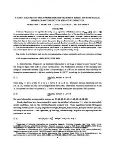
Fig. 1. The number of iterations for which both considered algorithms run depending on the value of the regularization parameter λ. The curve with the legend 𝑁 = 40 corresponds to the first scenario (𝑁 = 40, 𝑀 = 20, 𝐾 = 5, Gaussian 𝐀𝑜 ) and the curve with the legend 𝑁 = 200 corresponds to the second scenario (𝑁 = 200, 𝑀 = 80, 𝐾 = 20, Rademacher 𝐀𝑜 ).

9

(a)

(b) Fig. 2. The squared-ℓ2 -norm of the reconstruction error at different iterations when λ = 0.02 and ξ = 0.01 in the first (a) and the second (b) scenarios. The AD-CD and proposed algorithms converge to very similar values in both considered scenarios.

10

(a)

(b) Fig. 3. The converged squared-ℓ2 -norm of the reconstruction error for different values of λ when ξ = 0.01 in the first (a) and the second (b) scenarios. The results for the AD-CD and proposed algorithms are very similar for most values of λ in both considered scenarios.

11

(a)

(b) Fig. 4. The rates of false-negative and false-positive support-detection errors for different values of λ when ξ = 0.01 in the first (a) and the second (b) scenarios. In both scenarios, the false-negative errors of the AD-CD and proposed algorithms are almost identical for any value of λ in the considered range and the false-positive errors are almost identical when λ > 0.02.

12

(a)

(b) Fig. 5. The converged squared-ℓ2 -norm of the reconstruction error for different values of ξ when λ = 0.02 in the first (a) and the second (b) scenarios. The results for the AD-CD and proposed algorithms are very similar for all considered values of ξ in both considered scenarios.

13

Fig. 6. The average running time of each iteration of the AD-CD algorithm divided by the average running time of each iteration of the proposed algorithm for different values of λ in both considered scenarios.

14