Proceedings of the 2007 IEEE/RSJ International Conference on Intelligent Robots and Systems San Diego, CA, USA, Oct 29 - Nov 2, 2007
TuA3.4
Fast Reinforcement Learning Using Stochastic Shortest Paths for a Mobile Robot Wooyoung Kwon, Il Hong Suh, Sanghoon Lee and Young-Jo Cho little computation time per experience, they make extremely inefficient use of the data they gather and often require a great deal of experiences to achieve good learning performance. Therefore, some model-based reinforcement learning methods, which would require a state-transition probability function, can be efficient for practical cases of a mobile robot. These algorithms are especially important for the applications in which computation is considered to be cheap and real-world experience costly [7] [8] [9] [10]. In our previous works [11] [12], we proposed a MonteCarlo–based RL method involving a shortest path finding method to increase the probability of selecting the most appropriate behaviors as an effective learning technique. The main idea can be summarized as follows; Exploration for learning usually needs much cost, and may make the system be in danger; On the other hand, a shortest path finding method may usually cause a large number of computational or algorithmic complexity, but its cost is relatively low when compared with cost of exploration process in a real environment; By blending the shortest path finding method with an RL method, we can improve the learning performance in the sense of convergence speed. However, in our previous works, some weakness has been observed for learning state-action pairs in uncertain environment. Firstly, shortest path may be incorrect because an observed state is often confused by noisy sensor data. Secondly, state-transitions are often non-deterministic because of inaccurate sensor, uneven floor and/or anti-symmetric actuator. In a real environment, such a non-deterministic state-transition can have critical effects on finding the optimal path. To cope with the weakness of our previous approach, we reform our learning method by considering following perspectives; Firstly, the Long Term Memory(LTM) in our previous approach, which stores information on statetransitions composed of previous observed state, previous action and current state, is modified to a stochastic statetransition model. Secondly, a Stochastic Shortest Path(SSP) finding method is proposed to find the most relevant path in the stochastic state-transition model. To find an SSP, probabilistic cost function is defined by considering not only actual costs such as distances between two state or time during state-transition but also probabilities of state-transition. By applying probabilistic state-transition model and a stochastic shortest path-finding method, we will show implementation of both the learning speed and robustness of the proposing learning algorithm. The rest of this paper is organized as follows; A proposed learning algorithm combining Q-
Abstract— Reinforcement learning (RL) has been used as a learning mechanism for a mobile robot to learn state-action relations without a priori knowledge of working environment. However, most RL methods usually suffer from slow convergence to learn optimum state-action sequence. In this paper, it is intended to improve a learning speed by compounding an existing Q-learning method with a shortest path finding algorithm. To integrate the shortest path algorithm with Qlearning method, a stochastic state-transition model is used to store a previous observed state, a previous action and a current state. Whenever a robot reaches a goal, a Stochastic Shortest Path(SSP) will be found from the stochastic state-transition model. State-action pairs on the SSP will be counted as more significant in the action selection. Using this learning method, the learning speed will be boosted when compared with classical RL methods. To show the validity of our proposed learning technology, several simulations and experimental results will be illustrated.
I. I NTRODUCTION A mobile robot is often required to have an ability to learn what behaviors would be well suited for a given environmental situation for adaptation even with little or no priori task knowledge. To solve such an adaptation problem, many researchers have applied reinforcement learning to robot’s action adaptation on little or no priori knowledge [1] [2] [3]. Reinforcement learning [4] refers to a class of problems in machine learning which postulates an agent perceiving its current state and taking actions in an environment. The environment, in return, provides a reward, which can be positive or negative. Reinforcement learning algorithms attempt to find a policy for maximizing cumulative reward for the agent over the course of the problem. The reinforcement learning algorithms selectively retain the outputs that maximize the received reward over time. In the general case of the reinforcement learning problem, the actions of an agent determine not only its immediate reward, but also the next state of the environment [5]. Q-learning is widely used as a learning method involving little or no priori knowledge [6]. Q-learning is able to compare the expected utility of the available actions without requiring a model of the environment. Although many of these methods are guaranteed to eventually find optimal policies and use very The work reported in this paper was supported in part by “Embedded Component Technology and Standardization for URC” project of Ministry of Information and Communication. Wooyoung Kwon(e-mail:
[email protected]) and Young-Jo Cho(email:
[email protected]) are with Intelligent Robotics Division, Electronics and Telecommunications Research Institute, Daejon, Korea. And, Il Hong Suh(e-mail:
[email protected]) and Sanghoon Lee(e-mail:
[email protected]) are with Hanyang University, Seoul, Korea. All correspondences should be addressed to Il Hong Suh.
1-4244-0912-8/07/$25.00 ©2007 IEEE.
82
Initialize Q(s, a) arbitrarily Repeat (for each episode): Initialize previous observed state s Repeat (for each step of episode) Choose action a from previous observed state s using policy derived from Q (ε -greedy) Take action a, observe current reward r′ ,current state s′ Q(s, a) ← Q(s, a) + α [r′ + γ maxa′ Q(s′ , a′ ) − Q(s, a)] s ← s′ ; until s is terminal Fig. 1.
(a) all paths
Q-learning algorithm (b) shortest paths
learning with the stochastic shortest path finding method is explained in Sec. 2. Section 3 shows experimental setup for proposed learning algorithm. In Sec. 4, Experimental results of pushing a box into a goal position are presented. Finally, concluding remarks are given in Sec. 5.
Fig. 2.
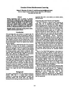
An example of shortest path finding
II. SSPQL : S TOCHASTIC S HORTEST PATHS BASED Q-L EARNING A. Q-learning Q-learning is a reinforcement learning technique to learn an action–value function that gives the expected utility of taking a given action in a given state [5]. Strength with Qlearning is that it is able to compare the expected utility of the available actions without requiring any model of environment. A summary of Q-learning algorithm is shown in Fig. 1. However, Q-learning may show some difficulties when applied to the reality: First, rewards may not be given immediately after an action is completed. Rewards are usually given after a goal is achieved by performing a sequence of actions. In general, this delayed reward causes the learning to be very time-consuming, or even to be not practical. To apply the Q-learning in real environment, it is necessary to reduce its long learning time mainly due to delayed rewards.
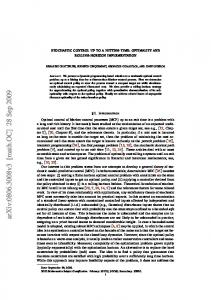
Fig. 3. Examples of state-transitions. State-transition probabilities and cost function for the case (b) are given as follows: P(si+1 |si , a1 ) = P(si−1 |si , a2 ) = 0.9, P(si |si , a1 ) = 0.1, P(si−1 |si , a2 ) = 0.9, P(si |si , a2 ) = 0.1, P(si+2 |si , a3 ) = 0.6, P(si+1 |si , a3 ) = 0.3, P(si |si , a3 ) = 0.1, P(si−2 |si , a4 ) = 0.6, P(si−1 |si , a4 ) = 0.3, P(si |si , a4 ) = 0.1, cost(si , a1 ) = cost(si , a2 ) = 1.0, cost(si , a3 ) = cost(si , a4 ) = 1.5
exploration strategies use shortest paths, the frequency of unnecessary exploration can be decreased. As a result, the performance of learning is expected to be improved. As the shortest path finding methods such as Dijkstra method and A* are based on deterministic environment, which is a process in perfect observation and deterministic statetransitions, it is not assured that they can be successfully applied to robotic work in real environment. Here, a very low-cost path with thin probability may be obtained by noisy sensor data and/or non-deterministic state-transitions. Given a shortest path finding method in a deterministic statetransition model, the path may be misunderstood as an optimal path. Once such a low-cost path with thin probability is stored in the deterministic state-transition model, continuous adverse effect can be observed on exploration. To avoid this, it is necessary to use a SSP finding method. Fig. 3 shows an example of state-transition under uncertain environment. As a result of action a1 , the probability of observing si+1 in the situation of si is 0.9 and the probability of observing si is 0.1. Similarly, as a result of the action a3 , the probability of observing si+2 is 0.6 and probability of observing other state is 0.4. The actual cost of an action can be regarded as the time to transit from a state to another. For example, let us find the shortest path from s1 to s5 ,
B. Stochastic Shortest Paths(SSP) in uncertain environment By the state-transition model of environment, an agent can predict how environment will respond to its action. Given a goal and a state-transition model, an agent can infer paths from a current state to a goal by backtracking transitions of states from the goal. This is the basic idea of shortest path finding methods. In comparison to Q-learning, an agent can follow the optimal path in one trial because the shortest path finding method requires no exploration. Our objective is to find shortest paths from all states to a single goal in a directed graph. Fig. 2-(b) shows the shortest paths of Fig. 2(a). Here, Dijkstra algorithm [13] is employed to find shortest paths. Dijkstra algorithm is a method to solve the singlesource shortest path problem which is the problem of finding a path between two vertices such that the sum of the nonnegative weights of its constituent edges is minimized. One of weaknesses of a shortest path finding method in a real world is to require a predefined state-transition model for working environment. Such a requirement can be mitigated by combining the shortest path finding method with Qlearning which does not require a priori knowledge. If
83
Initialize Q(s, a) Initialize a state-transition model P(s′ |s, a) Do until learning end Do until a robot reaches a goal Observe a current state s’ and reward signal r’ Choose action a s.t. a = argmaxa′ [Q(s′ , a′ ) + wsspVssp (s′ , a′ )] togethter with ε -greedy policy Execute action a Update Q-Value with Q(s, a) ← Q(s, a) + α [r′ + γ maxa′ Q(s′ , a′ ) − Q(s, a)] Update state-transition model P(s′ |s, a) S, A ⇐= stochastic shortest paths from all state to goal state using Dijkstra algorithm Update Vssp (s, a) S, A : states and actions consisting of stochastic shortest paths
which cost function includes a distance and a time in the deterministic environment as shown in Fig. 3-(a). In this case, shortest path is given as (s1 , a3 ) ⇒ (s3 , a3 ) ⇒ s5 . However, when considering stochastic state-transitions as in Fig. 3(b), the action a3 may not be the best choice because a3 causes the next state to be more uncertain than a1 does. To be more specific, firstly, by selecting a3 , the sequence may be (s1 , a3 ) ⇒ (s2 , a3 ) ⇒ (s3 , a3 ) ⇒ s5 and its cost is 4.5. Secondly, by selecting a1 , the sequence may be (s1 , a1 ) ⇒ (s2 , a1 ) ⇒ (s3 , a1 ) ⇒ (s4 , a1 ) ⇒ s5 and its cost is 4.0. In this example, selecting a3 requires more cost. Unfortunately, the expected cost cannot be exactly computed because state-transitions are non-deterministic in real environment, and the computation of the expected cost requires a lot of recursive computations. Therefore, the expected cost here is approximately computed by both using distance between states and probability of state-transition. When uncertainty of a state-transition is low, the difference between the expected and actual cost will be small. On the contrary, the difference is large, when uncertainty is high. Thus, optimal paths in real environment should be varied by the probability of state-transitions. The expected cost of a state-transition from state s to s′ is defined as ¶−ω µ#of action ′ , P(s |s, a ) cost ∗ (s, s′ ) = cost(s, s′ ) i ∑
Fig. 4.
(1)
where ω is a weight to reflect uncertainty and cost(s, s′ ) is a pre-defined real cost function such as a minimum distance between two states. The equation of state-transition probability can be defined as
t−1 ,at−1 ,st ) N(st−1 ,at−1 )
µ (µ ≈ 0)
if N(st−1 , at−1 ) 6= 0 if N(st−1 , at−1 ) = 0,
Shortest
Path(SSP)-based
(3)
a = argmaxa′ [Q(s′ , a′ ) + wsspi (s′ , a′ )Vssp (s′ , a′ )].
(4)
Here, wsspi (s, a) is a weight value of of SSP. Algorithm of SSPQL is summarized in Fig. 4. D. Convergence, Optimality, and Computational Complexity of the proposed algorithm
(2)
In classical Q-learning methods, convergence and optimality have been formally proved with appropriate parameters in the situation of Markov Decision Processs(MDPs) [14] under the following conditions; bounded rewards |r| ≤ const, learning rates 0 ≤ α ≤ 1, and decreasing learning rate over time. As in Q-learning, our SSPQL can be shown to have convergence and optimality of following hold:
where N(st−1 , at−1 , st ) is the number of observations of st followed by action at−1 in a state st−1 and µ is a small positive value; Ncur (st−1 , at−1 ) is the frequency of action at in a state st . C. Stochastic (SSPQL)
Vssp (si1 , a j1 ) P(si2 |si1 , a j1 )P(si3 |si2 , a j2 ) . . . P(sG |siN , a jN ) if si1 , a j1 in stochastic shortest paths = 0 else.
In (3), si1 , si2 , . . . , siN are states on stochastic shortest path from si1 to a goal state sG and a j1 , a j2 , . . . , a jN−1 are actions with maximum transition probability between the states: For example, an action a j1 is the action with maximum probability from si1 to si2 . If the uncertainty of state-transitions is small, Vssp will be close to 1. Otherwise, it will be close to 0. In summary, an optimal policy function can be defined as
i=0
P(st |st−1 , at−1 ) = ( N(s
SSPQL algorithm
0 ≤ wsspi (s, a) ≤ 1, lim wsspi (s, a) = 0, ∀s, a.
Q-Learning
i→∞
(5)
In (5), wsspi (s, a) is the weightings for the action a of the ith trials at state s. Under the conditions in (5), as i goes to infinity, 2nd and 3rd terms of (4) become null. Thus, (4) will eventually consist of Q-value and a random number. This is the same form of optimal action-value function for Qlearning. Thus, SSPQL can have optimal convergence property as Q-learning. It is remarked that wsspi (s, a) = N(s, a)−w is a simple equation to satisfy (5). SSP-value is designed to put a relatively large effect on the action selection at early stages of learning. As the number of episodes are increased, effects of the term will be diminished. In this condition, SSP plays a role of assigning values believed to be close to an
To integrate SSP with the Q-learning method, a previous observed state, a previous action and a current state will be stored in a probabilistic state–transition model at every step. After one episode ends, shortest paths reaching a goal state from every states can be found by using Dijkstra algorithm with a cost function of (1) in the stochastic state-transition model. By increasing probability of selecting the actions with maximum transition-probability between states in exploration strategy, the speed of convergence can be improved. The amount of probability of selecting actions can be computed by
84
Fig. 5.
A Photo of our experimental mobile robot
Fig. 6.
unknown optimal Q-value at early stages of learning, which is expected to boost learning speed of SSPQL. Next, computational complexity of SSPQL can be computed by considering complexity of finding a shortest path and computation of Vssp to reach a goal state. First of all, running time of Dijkstra algorithm is O(n2 ) on a graph with n nodes and m edges. In our SSP, a node is mapped into a state, and an edge which is a transition between two nodes is mapped into a state-transition by an action. Thus, the number of nodes equals the number of state, and the number of edges equals the number of vector product of states and actions. For sparse graphs with edges much less than n2 , Dijkstra algorithm can be implemented much efficiently by storing the graph in the form of adjacency lists and using a binary or a Fibonacci heap as a priority queue to implement the ExtractMin function [13]. The algorithm requires O((m + n) log n) time in case of a binary heap, while it is O(m + n log n) in case of a Fibonacci heap. So, we can improve the computational complexity of SSP algorithm into O(m + n log n). Next, computational complexity of Vssp (s, a) as shown in (3) is O(n2 ). However, by ignoring state-action pairs which have low probability, the computational complexity can be decrease to O(n log n). Thus, total computational complexity of stochastic shortest path finding process is O(m + 2n log n).
Fig. 7.
A task description for box-pushing task
Initial positions of robot with respect to the box and goal
a goal. To make our task learning more effective, the task is decomposed into more detailed four sub-tasks: search, approach, turn, and push sub-tasks. Firstly, the robot searches for positions of the box and the goal by using its camera and IR scanner. Secondly, the robot moves to the area in which the robot can get a reward as depicted in Fig. 6-(b). Thirdly, the robot aligns itself with the box and the goal so that they are in a line as shown Fig. 6-(c). Finally, the robot pushes the box into the goal. For subtasks of ‘search’ and ‘push’, we designed and used rules and thus, those two tasks need not to get any more learning. The sub-tasks of ‘approach’ and ‘turn’ are now being learned from the scratch. C. States and primitive actions To apply reinforcement learning to the real robot task, it is necessary to design a discrete set of environmental states, primitive actions, and scalar reinforcement signals. If we define a state in such a way that the state implies object position with respect to the robot position in Cartesian coordinate, state-transitions would be too complex to manage. This causes learning process to be hard or to be a lot of time consuming process. Here, to reduce the number of states and to simplify state-transitions, we will set up a new coordinate system such that a box is located at the center of the coordinate, and the goal is faced to the 0◦ direction as depicted in Fig. 8. Transformed positions of the box, goal, and robot can be computed by
III. E XPERIMENT A. Experimental Setup To show the validity of our SSPQL algorithm, a task of pushing a box into a goal is considered for a mobile robot as shown in Fig. 5, where the robot has a differential-drive locomotion, a ring of 16 sonar sensors, a single CCD camera, and an Infra-Red(IR) range scanner to measure distances from objects and wall in the world. Higher-level features such as relative positions of a box and a goal are computed from raw distance information and color segmentation of camera image. Due to the camera with restricted field of view, our robot is required to estimate locations for out-of-sight-objects. A Bayesian filter is used to estimate the posterior probability density locations of objects over the state–space on the data [15].
xgoalnew = (xgoal − ∆x) cos(∆θ ) − (ygoal − ∆y) sin(∆θ ), ygoalnew = (xgoal − ∆x) sin(∆θ ) + (ygoal − ∆y) cos(∆θ ), xrobotnew = (−∆x) cos(∆θ ) − (−∆y) sin(∆θ ), yrobotnew = (−∆x) sin(∆θ ) + (−∆y) cos(∆θ ),
(6)
θrobotnew = ∆θ ,
B. Task Description
¡ ¢ where ∆θ = − arctan (ygoal − ybox )/(xgoal − xbox ) , ∆x = −xbox , and ∆y = −ybox . Here, xgoal and ygoal imply x and y
To show the validity of our proposed reinforcement learning method, there is given the task of pushing a box into
85
Fig. 9.
Number of steps in ‘approach’ sub-task of Fig. 5-(a)
Fig. 10.
Number of steps in ‘approach’ sub-task of Fig. 5-(b)
(a) Description of 36 states of S pos
(b) Description of 12 states of Sheading S ⇐= S pos × Sheading Fig. 8.
Definition of state space
coordinate of the goal in world cartesian space, respectively. And, xbox and ybox imply x and y coordinate of the box in world cartesian space, respectively. S pos is a space of pose-dependent states. S pos is designed to have 36 different states determined by 12 robot orientations as well as 3 distances from a box to a goal as shown in Fig. 8-(a). Sheading is a state space of robot heading angle, and is here designed to have 12 states as shown in Fig. 8(b). The xrobotnew and yrobotnew is used to determine a state in S pos , and θrobotnew is used to determine a state in Sheading . Whole state space is defined as the product space of S pos and Sheading . Next, four primitive actions are defined: ‘move forward by 0.3m’, ‘move backward by 0.2m’, ‘turn 30o ’, ‘turn −25o ’. A reward signals is generated whenever the robot arrives at the state of S pos marked “A” and Sheading =0o as shown in Fig. 8-(a).
as in Fig. 7-(a). The number of steps of Q-learning is decreased after the ninth episode, because propagation of a reward signal by Q-value-update is slow. This is not because the state-space is large, but because state-transitions are stochastic so that the optimal path is not clear. However, the number of steps of SSPQL is decreased more quickly than that of Q-learning. Fig. 10 shows the number of steps per episode with the initial configuration set as shown in Fig. 7-(b). This figure also illustrates that our SSPQL method makes the learning process much faster than Q-learning. From the above results, it is apparent that the speed of propagation of reward signals in SSPQL is much faster than that of Q-learning. This is because the shortest path finding
D. Experimental and Simulation Results We applied our SSPQL method to the box-pushing task with two initial positions as shown in Fig. 7. For comparison, Q-learning approach was also experimented in simulations. During all experiments, parameters for Q-function are chosen as γ = 0.8, α = 0.8 and ε = 0.1. And the weight values of SSP is given as wssp = 1.5. 1) Simulational results: To simulate environment and a real robot, we use an open source simulator, Player and Stage [16]. Fig. 9 shows the number of steps per episode of Qlearning and our SSPQL method with initial configuration
Fig. 11.
86
Number of steps in ‘turn’ sub-task
Fig. 14.
Fig. 12.
Trajectory of a robot
when state transitions are stochastic. However, our SSPQL needs to be more improved by considering the followings; Firstly, it requires a lot of memory to store state-transition probabilities and stochastic shortest paths. Secondly, it needs more computations to find shortest path. As a conclusion, SSPQL would be suitable for fast learning of a task in real environment where state-transitions are non-deterministic and a robot has to be operating under some restricted resources. Here, time is considered as a restricted resource, since a lot of computational time is not usually allowed in real time applications
‘approach’ sub-task of real robot
R EFERENCES
Fig. 13.
[1] C. M. Witkowski, “Schemes for learning and behaviour: A new expectancy model,” Ph.D. dissertation, University of London, 1997. [2] M. Humphrys, “Action selection methods using reinforcement learning,” Ph.D. dissertation, University of Cambridge, 1996. [3] I. H. Suh, S. Lee, B. O. Kim, B. J. Yi, and S. R. Oh, “Design and implementation of a behavior-based control and learning architecture for mobile robots,” in Proceedings of IEEE/RSJ International Conference on Robotics an Autonomous, 2003. [4] R. C. Arkin, “Steps towards artificial intelligence,” in Proceedings of the Institute of Radio Engineers, 1961. [5] R. Sutton and A. Barto, Reinforcement Learning. MIT Press, 1996. [6] C. Watkins, “Learning from delayed rewards,” Ph.D. dissertation, University of Cambridge, 1989. [7] R. Sutton, “Integrated architectures for learning, planning, and reacting based on approximating dynamic programming,” in Proceedings of the Seventh International Conference on Machine Learning, 1990. [8] A. W. Moore and C. G. Atkeson, “Prioritized sweeping: Reinforcement learning with less data and less real time,” Machine Learning, vol. 13, pp. 103–130, 1993. [9] M. Wiering and J. Schmidhuber, “Fast online Q(λ ),” Machine Learning, vol. 33, pp. 105–115, 1998. [10] J. Schmidhuber, “Exploring the predictable,” in Advances in Evolutionary Computing, A. Ghosh and S. Tsuitsui, Eds. Kluwer, 2002. [11] W. Y. Kwon, S. H. Lee, and I. H. Suh, “A reinforcement learning approach involving a shortest path finding algorithm,” in Proceedings of IEEE/RSJ International Conference on Intelligent Robots and Systems, 2003, pp. 27–31. [12] I. H. Suh, S. Lee, W. Kwon, and Y. J. Cho, “Learning of action patterns and reactive behavior plans via a novel two-layered ethologybased action selection mechanism,” in Proceedings of IEEE/RSJ International Conference on Intelligent Robots and Systems, 2005, pp. 1232–1238. [13] R. Neapolitan, Foundation of algorithms : using C++ pseudocode. Jones and Bartlett Publishers, 1998. [14] C. J. C. H. Watkins and P. Dayan, “Technical note q-learning.” Machine Learning, vol. 8, pp. 279–292, 1992. [15] A. Doucet, N. de Freitas, and N. Gordon, Sequential Monte Carlo in Practice. Springer-Verlag, 2001. [16] B. P. Gerkey, R. T. Vaughan, and A. Howard, “The player/stage project: Tools for multi- robot and distributed sensor systems’,” in Proceedings of IEEE/RSJ International Conference on Robotics and Automation, 2003, pp. 317–323.
‘turn’ sub-task of real robot
method is a batch process with a given state-transition model. Fig. 11 shows the result of ‘turn’ sub-tasks. In this result, the convergence speed of both Q-learning and SSPQL are almost the same, since the state space is small and statetransitions is simple. The state space of ‘turn’ sub-task is restricted in region “A” as shown in Fig. 8-(a) such that the number of state-space is 24 (2×12, 2 for positions and 12 for directions). Finally, Fig. 14 shows the comparison of trajectory of a robot made by SSPQL and hand-coded optimal rules in case of ‘approach’ sub-task. From this result, it seems that there is a negligible difference between learned rules by SSPQL and hand-coded rule. 2) Experimental results for a real-robot: Fig. 12 and Fig. 13 show the results of ‘approach’ and ‘turn’ subtasks for a real robot. Experimental results are similar to those of simulations, because simulational environement was prepared to be close to the real environment. It is observed that there was a little increase of steps per episode for the experiment due to more noisy sensor signals and/or more non-deterministic floor characteristics than we expected in simulations. IV. C ONCLUSION We proposed a Stochastic Shortest Path-based Q-Learning (SSPQL) method. One advantage of SSPQL method is the improvement of convergence speed when compared to model-free approaches such as Q-learning. The experimental results show that SSPQL is much faster than Q-learning. Another advantage of SSPQL is that it works well even
87