Hard real-time systems are those that are specified in terms of strong timing ... to implementing redundancy in hard real-time systems so that their fault resilience ...
Fault Tolerance in Fixed-Priority Hard Real-Time Distributed Systems
George Marconi de Ara´ ujo Lima
Submitted for the degree of Doctor of Philosophy
University of York Department of Computer Science May 2003
To my wife Verˆonica
Abstract Hard real-time systems are those that are specified in terms of strong timing constraints. They are often involved in critical activities, where human lives may sometimes be at stake. These characteristics emphasise the need for making the services provided by this kind of system fault-tolerant. However, doing so is not simple. It involves implementing redundancy into the system so that if a system component is faulty others can provide the expected service. The extra computation due to these redundant components, in turn, may affect the system correctness since its timing constraints may be violated. This thesis contributes to this research area by describing some approaches to implementing redundancy in hard real-time systems so that their fault resilience is optimised. It considers the implementation of both passive and active redundancy in a distributed architecture, where a set of fixed-priority scheduled tasks is statically allocated to each node of the system. Passive redundancy is implemented by releasing alternative tasks upon error detection. Active redundancy is due to task replication in different nodes, where agreement on the produced results is used to guarantee the consistency of distributed computation. As for the execution of alternative tasks, the research work presented in this thesis is focused on determining the best priority assignment policies for fault tolerance purposes. One of the results of the thesis is the description of an approach that assigns priorities to alternative tasks so that the fault resilience of the task set is optimised. This approach conveys not only a priority assignment policy but also schedulability analysis, with which it is possible to check whether task sets may violate their timing constraints under a given fault assumption. An assessment of the proposed approach is also provided. For supporting distributed agreement, two consensus protocols are proposed. These protocols are designed to take advantage of some properties of CAN, a priority-oriented communication network, which is widely used in hard real-time systems. It is demonstrated that achieving consensus in CAN without relying on strong timing assumptions is possible. The fault resilience of both protocols is optimal in terms of the number of tolerated crashes. These characteristics means that the proposed protocols compare favourably with other approaches usually employed to support hard real-time systems.
Contents
Abstract
3
Acknowledgements
17
Declaration
19
1 Introduction
21
1.1
The Target System . . . . . . . . . . . . . . . . . . . . . . . . . . . . .
22
1.1.1
Redundant Components . . . . . . . . . . . . . . . . . . . . . .
22
1.1.2
Computation Timeliness . . . . . . . . . . . . . . . . . . . . . .
23
1.2
The Thesis Goal
. . . . . . . . . . . . . . . . . . . . . . . . . . . . . .
25
1.3
The Thesis Structure . . . . . . . . . . . . . . . . . . . . . . . . . . . .
25
2 Fault Tolerance in Real-Time Systems
27
2.1
An Informal Introduction to Correctness . . . . . . . . . . . . . . . . .
28
2.2
Real-Time Systems . . . . . . . . . . . . . . . . . . . . . . . . . . . . .
29
2.2.1
Structuring the Computation . . . . . . . . . . . . . . . . . . .
30
2.2.2
Modelling Task Activation
33
5
. . . . . . . . . . . . . . . . . . . .
CONTENTS
2.3
6
The Scheduling Problem . . . . . . . . . . . . . . . . . . . . . . . . . .
33
2.3.1
Fixed Priority Scheduling . . . . . . . . . . . . . . . . . . . . .
35
Fault Tolerance . . . . . . . . . . . . . . . . . . . . . . . . . . . . . . .
37
2.4.1
Faults . . . . . . . . . . . . . . . . . . . . . . . . . . . . . . . .
38
2.4.2
Failures . . . . . . . . . . . . . . . . . . . . . . . . . . . . . . .
39
2.4.3
Approaches to Fault Tolerance
. . . . . . . . . . . . . . . . . .
39
2.5
Distributed Systems . . . . . . . . . . . . . . . . . . . . . . . . . . . .
41
2.6
Fault-Tolerant Real-Time Systems
. . . . . . . . . . . . . . . . . . . .
43
2.6.1
Supporting Passive-Redundancy Based Techniques . . . . . . .
43
2.6.2
Supporting Active-Redundancy Based Techniques
. . . . . . .
47
2.7
The Consensus Problem . . . . . . . . . . . . . . . . . . . . . . . . . .
49
2.8
Summary . . . . . . . . . . . . . . . . . . . . . . . . . . . . . . . . . .
52
2.4
3 Computational Model and Initial Concepts 3.1
3.2
3.3
The Computational Model
55
. . . . . . . . . . . . . . . . . . . . . . . .
56
3.1.1
The Intra-Node Model . . . . . . . . . . . . . . . . . . . . . . .
58
3.1.2
The Inter-Node Model . . . . . . . . . . . . . . . . . . . . . . .
60
Response Time Analysis for Fault Tolerance . . . . . . . . . . . . . . .
65
3.2.1
Response Time Analysis in Fault-Free Scenarios . . . . . . . . .
66
3.2.2
Response Time Analysis in Fault Scenarios
. . . . . . . . . . .
67
3.2.3
On the Priorities of Alternative Tasks
. . . . . . . . . . . . . .
68
Consensus in CAN . . . . . . . . . . . . . . . . . . . . . . . . . . . . .
70
CONTENTS
3.4
7
3.3.1
The Consequences of the Inconsistent Scenarios . . . . . . . . .
71
3.3.2
Software-Based Solutions
. . . . . . . . . . . . . . . . . . . . .
72
3.3.3
Hardware-Based Solutions . . . . . . . . . . . . . . . . . . . . .
74
Summary . . . . . . . . . . . . . . . . . . . . . . . . . . . . . . . . . .
75
4 Response Time Analysis for Fault Tolerance Purposes 4.1
4.2
77
Raising Priorities of Alternative Tasks . . . . . . . . . . . . . . . . . .
79
4.1.1
Priority Configuration . . . . . . . . . . . . . . . . . . . . . . .
79
4.1.2
Effects of Higher Priority Alternative Tasks . . . . . . . . . . .
80
4.1.3
Interfering Task Sets . . . . . . . . . . . . . . . . . . . . . . . .
81
Response Time Analysis Derivation
. . . . . . . . . . . . . . . . . . .
82
4.2.1
Considering only External Errors . . . . . . . . . . . . . . . . .
83
4.2.2
Considering Internal Errors . . . . . . . . . . . . . . . . . . . .
86
4.2.3
Worst-Case Response Time . . . . . . . . . . . . . . . . . . . .
89
4.2.4
Incorporating Release Jitter and Blocking . . . . . . . . . . . .
91
4.3
Some Comments on the Use of TE
. . . . . . . . . . . . . . . . . . . .
94
4.4
An Illustrative Example . . . . . . . . . . . . . . . . . . . . . . . . . .
95
4.5
Summary . . . . . . . . . . . . . . . . . . . . . . . . . . . . . . . . . .
98
5 Assigning Priorities to Alternative Tasks 5.1
99
The Priority Configuration Search Method . . . . . . . . . . . . . . . . 100 5.1.1
Dominant Tasks
. . . . . . . . . . . . . . . . . . . . . . . . . . 101
5.1.2
Search Graph . . . . . . . . . . . . . . . . . . . . . . . . . . . . 104
CONTENTS
5.1.3
8
Search Path
. . . . . . . . . . . . . . . . . . . . . . . . . . . . 106
5.2
Implementing the Method . . . . . . . . . . . . . . . . . . . . . . . . . 108
5.3
Correctness and Complexity of the Algorithm . . . . . . . . . . . . . . 112
5.4
Assessment of Effectiveness . . . . . . . . . . . . . . . . . . . . . . . . 114
5.5
5.4.1
Specification of the Task Set Generation Procedure . . . . . . . 115
5.4.2
Assessment of Schedulability under Errors . . . . . . . . . . . . 120
5.4.3
Assessment of Fault Resilience
. . . . . . . . . . . . . . . . . . 122
Summary . . . . . . . . . . . . . . . . . . . . . . . . . . . . . . . . . . 127
6 A Priority-Based Consensus Protocol
129
6.1
On Communication Synchronism and Fault Resilience
6.2
Assumptions on the System Synchronism
6.3
6.4
. . . . . . . . . 131
. . . . . . . . . . . . . . . . 133
6.2.1
Local Clocks . . . . . . . . . . . . . . . . . . . . . . . . . . . . . 133
6.2.2
Processing . . . . . . . . . . . . . . . . . . . . . . . . . . . . . . 133
6.2.3
Communication . . . . . . . . . . . . . . . . . . . . . . . . . . . 134
The Timed Consensus Protocol . . . . . . . . . . . . . . . . . . . . . . 136 6.3.1
Protocol Overview . . . . . . . . . . . . . . . . . . . . . . . . . 136
6.3.2
Illustrative Description
. . . . . . . . . . . . . . . . . . . . . . 139
Determining the Round Duration . . . . . . . . . . . . . . . . . . . . . 142 6.4.1
Case 1: Two Processes and Synchronous Rounds
. . . . . . . . 143
6.4.2
Case 2: Two Processes and Asynchronous Rounds . . . . . . . . 144
6.4.3
Case 3: Three Processes and Asynchronous Rounds . . . . . . . 146
CONTENTS
6.4.4
9
The General Case . . . . . . . . . . . . . . . . . . . . . . . . . . 148
6.5
Proof of Correctness . . . . . . . . . . . . . . . . . . . . . . . . . . . . 152
6.6
Complexity Analysis . . . . . . . . . . . . . . . . . . . . . . . . . . . . 154
6.7
Summary . . . . . . . . . . . . . . . . . . . . . . . . . . . . . . . . . . 155
7 An Ordering-Based Consensus Protocol 7.1
157
The Consensus Protocol . . . . . . . . . . . . . . . . . . . . . . . . . . 159 7.1.1
Protocol Overview . . . . . . . . . . . . . . . . . . . . . . . . . 160
7.1.2
Illustrative Description
7.1.3
A Special Case: Speakers Only . . . . . . . . . . . . . . . . . . 166
. . . . . . . . . . . . . . . . . . . . . . 162
7.2
Proof of Correctness . . . . . . . . . . . . . . . . . . . . . . . . . . . . 166
7.3
Complexity Analysis . . . . . . . . . . . . . . . . . . . . . . . . . . . . 169
7.4
7.3.1
Theoretical Analysis . . . . . . . . . . . . . . . . . . . . . . . . 169
7.3.2
Empirical Analysis . . . . . . . . . . . . . . . . . . . . . . . . . 173
Summary . . . . . . . . . . . . . . . . . . . . . . . . . . . . . . . . . . 179
8 Dealing with Consensus Delays
181
8.1
Optimistic Release of Tasks . . . . . . . . . . . . . . . . . . . . . . . . 182
8.2
An Illustrative Example . . . . . . . . . . . . . . . . . . . . . . . . . . 185
8.3
8.2.1
On the Performance of τ5c . . . . . . . . . . . . . . . . . . . . . 185
8.2.2
On the Fault Resilience of the Task Set
. . . . . . . . . . . . . 186
Summary . . . . . . . . . . . . . . . . . . . . . . . . . . . . . . . . . . 187
9 Conclusion
189
CONTENTS
10
9.1
Summary of the Main Contributions . . . . . . . . . . . . . . . . . . . 189
9.2
Possible Directions for Further Research . . . . . . . . . . . . . . . . . 191
A An Alternative Fault Resilience Metric A.1 Schedulability Analysis
195
. . . . . . . . . . . . . . . . . . . . . . . . . . 196
A.1.1 Considering only External Errors . . . . . . . . . . . . . . . . . 198 A.1.2 Considering Internal Errors . . . . . . . . . . . . . . . . . . . . 199 A.1.3 An Illustrative Example . . . . . . . . . . . . . . . . . . . . . . 202 A.2 Priority Assignment and Evaluation
. . . . . . . . . . . . . . . . . . . 206
A.2.1 Redefinitions of some Concepts . . . . . . . . . . . . . . . . . . 206 A.2.2 The Algorithm and Results of Experiments
. . . . . . . . . . . 208
A.3 Summary . . . . . . . . . . . . . . . . . . . . . . . . . . . . . . . . . . 212
List of Figures
2.1
The life cycle of real-time tasks. . . . . . . . . . . . . . . . . . . . . . .
31
2.2
Different kinds of failures and their relationships. . . . . . . . . . . . .
40
3.1
Illustration of the assumed architecture. . . . . . . . . . . . . . . . . .
57
3.2
Priority assignment in fault-scenarios. . . . . . . . . . . . . . . . . . . .
69
3.3
Inconsistent scenarios as an impairment of consensus.
. . . . . . . . .
71
4.1
Worst-case execution scenarios. . . . . . . . . . . . . . . . . . . . . . .
81
4.2
Γ subsets with respect to task τi . . . . . . . . . . . . . . . . . . . . . .
82
4.3
Illustration of the derivation of Riint (x, TE ).
86
4.4
Illustration of R3int (x, TE ) relating to table 4.1.
5.1
Illustration of the meaning of dominant tasks. . . . . . . . . . . . . . . 102
5.2
Scenarios where the improvement condition does not hold. . . . . . . . 104
5.3
The search graph for a set of 3 tasks.
5.4
The search path for the task set given by table 3.1. . . . . . . . . . . . 107
5.5
A search path which contains the vertex labelled with the optimal priority configuration.
. . . . . . . . . . . . . . . . . . . . . . . . . . . .
97
. . . . . . . . . . . . . . . . . . 105
. . . . . . . . . . . . . . . . . . . . . . . . . . . . 109
11
LIST OF FIGURES
12
5.6
The optimal priority configuration search algorithm.
. . . . . . . . . . 110
5.7
The typical distribution of the processor utilisation of the generated task sets. . . . . . . . . . . . . . . . . . . . . . . . . . . . . . . . . . . . . . 118
5.8
Schedulability of task sets in fault-free and in fault scenarios.
. . . . . 119
5.9
Percentage of non-fault-tolerant task sets made fault-tolerant by carrying out the proposed approach. . . . . . . . . . . . . . . . . . . . . . . 121
5.10 Improvement in terms of fault resilience measured as obtained reduction of TE . Fixing the size of task sets n = 10 and varying fC .
. . . . . . . 124
5.11 Improvement in terms of fault resilience measured as obtained reduction of TE . Fixing the size of task sets n = 10 and considering higher values for fC .
. . . . . . . . . . . . . . . . . . . . . . . . . . . . . . . . . . . 125
5.12 Improvement in terms of fault resilience measured as obtained reduction of TE . Fixing fC = 1 and varying the size of task sets n. . . . . . . . . 126 6.1
Three scenarios illustrating increasing fault resilience when communication synchrony is relaxed. . . . . . . . . . . . . . . . . . . . . . . . . . 131
6.2
A priority-based consensus protocol.
6.3
Two execution scenarios for the consensus protocol described in figure 6.2.140
6.4
Achieving consensus despite inconsistent message duplication. . . . . . 141
6.5
Achieving consensus despite non-synchronous execution of the protocol. 142
6.6
The value of ∆ in cases where processes execute the rounds of the consensus protocol synchronously.
6.7
. . . . . . . . . . . . . . . . . . . 137
. . . . . . . . . . . . . . . . . . . . . . 144
The value of ∆ in cases where processes execute the rounds of the consensus protocol asynchronously. . . . . . . . . . . . . . . . . . . . . . . 145
6.8
The round duration for three processes considering asynchronous rounds. 147
6.9
Illustration of agreement despite asynchronous execution. . . . . . . . . 150
LIST OF FIGURES
13
7.1
The message-ordering-based consensus protocol.
. . . . . . . . . . . . 160
7.2
The behaviours of speakers and listeners under fault scenarios. . . . . . 163
7.3
The effect of θ on the waiting time.
7.4
The consensus protocol of figure 7.1 when ∆ = 0 and/or θ = 1.
7.5
Examples of scenarios relating to the execution of the protocol of figure
. . . . . . . . . . . . . . . . . . . 165 . . . . 166
7.1. . . . . . . . . . . . . . . . . . . . . . . . . . . . . . . . . . . . . . . 170 7.6
Effects of varying θ in terms of number of rounds and messages. . . . . 176
7.7
Effects of varying ∆ in terms of number of rounds and messages. . . . . 177
7.8
Average time spent per correct process. . . . . . . . . . . . . . . . . . . 178
8.1
Optimistic approach to decreasing the waiting time of any consensus task τic . . . . . . . . . . . . . . . . . . . . . . . . . . . . . . . . . . . . 183
A.1 A scenario where τ1 and τ2 are schedulable despite two internal errors in τ3 : τ1 and τ2 arrive just after the τ 3 is released (the worst-case).
. . 196
A.2 Procedure to determine the values of Ni0 and Ni1 such that the worst-case scenario is represented and equation (A.1) holds.
. . . . . . . . . . . . 201
A.3 Two possible fault scenarios for task τ3 and NE = 2. . . . . . . . . . . . 205 A.4 The optimal priority configuration search algorithm.
. . . . . . . . . . 209
A.5 Improvement in terms of fault resilience measured as obtained increase of NE . Fixing the size of task sets n = 10 and varying fC . . . . . . . . 210
List of Tables
2.1
A classification of real-time scheduling.
3.1
A task set and the derived worst-case response times.
4.1
The effects of raising priorities of alternative tasks for different priority configurations.
5.1
. . . . . . . . . . . . . . . . . . . . . . . . . .
. . . . . . . . . . . . . . . . . . . . . . . . . . . . . . .
34 68
95
Worst-case response times due to internal and external errors when TE = Te (x) − 1. . . . . . . . . . . . . . . . . . . . . . . . . . . . . . . . . . . 103
5.2
An example of a task set which can have high gains in fault resilience. . 127
8.1
A task set with 6 tasks and their worst-case response times (in bold). . 184
8.2
Worst-case response times when τ5c starts executing earlier (all errors in τ5 due to inconsistent scenarios).
8.3
. . . . . . . . . . . . . . . . . . . . . 186
The worst-case response times when τ5c starts executing earlier.
. . . . 187
A.1 An illustrative task set and the values of worst-case response times. . . 202 A.2 The example of table 5.2 under the revised approach. . . . . . . . . . . 211
15
Acknowledgements I am very grateful to my supervisor, Alan Burns, whose guidance, friendship and encouragement were of paramount importance in this work. The friendly working atmosphere provided by the members of the Real-Time Research group has made four years of hard work not so hard. I am grateful to all the members of the group for this. I wish to acknowledge the Brazilian funding agency CAPES for providing the financial support. Without this help coming to York would not have been possible. Many thanks to Malcolm Wren, who helped me to solve many of my problems with the English language. My gratitude goes also to Tse Lin, Guiem Bernat, Renato Krohling and Carol Burns for their helpful comments about some parts of the thesis and to Ian Broster for our fruitful discussion about CAN. There are many friends I would like to thank. Their support was very important during my stay in York. Thanks to Olga Miranda and Tse Lin, Pamela Luna and Guiem Bernat, Eraldo Ribeiro, Carmem and Roger Mackle, Renato Krohling, Filo Ottaway, Eduarda Paz and Guilherme Campos, Karin and Jose Jara, Ariane Mildenberg and Malcolm Wren. Many thanks also to my colleagues at LaSiD/UFBA in Brazil. Specially Fabiola Greve, Raimundo Macˆedo, Fl´avio Assis and Aline Andrade, who kept motivating and encouraging me all along. I would like to express my sincere gratitude to those who, despite their physical distance, have enabled me to feel so close to them during all these years. Thanks to my parents, Grinaldo and Iva Lima, and to my sisters, Ivana and Itana Lima and M´ıriam Carvalho, for their unshakable belief in me. To my family-in-law, Dem´ostenes, Janet, C´audia, Paulo, Roberta and Nilce Almeida, and Marcelo Carvalho, my many thanks
17
Acknowledgements
18
for all your support and affection. I owe Verˆonica a great deal. She shared each minute of this journey with me. Her love has been my source of strength.
Declaration I declare that the research work presented in this thesis is original unless otherwise indicated in the text. Some parts of this work have appeared in or have been submitted to scientific publications. A preliminary version of the material described in chapter 4 has been published as the paper “An Effective Schedulability Analysis for Fault-Tolerant Hard Real-Time Systems” [57], which appeared in the Proceedings of the Thirteen Euromicro Conference on Real-Time Systems in 2001. Chapters 4 and 5 are the basis of the paper “An Optimal Fixed-Priority Assignment Algorithm for Supporting Fault Tolerant Hard Real-Time Systems” [60], accepted for publication in the IEEE Transaction on Computers. The initial ideas presented in chapter 6 have been discussed in the Proceedings of the Work-in-Progress Session of the Twenty Second Real-Time Systems Symposium, 2001, as the paper “A Timely Distributed Consensus Solution in a Crash/OmissionFault Environment” [56]. The material of chapter 7 was developed based on the paper “Timing-Independent Safety on Top of CAN” [58], published in 2002 in the Proceedings of the First International Workshop on Real-Time LANs in the Internet Age. The main result of this chapter is published in the Proceedings of the Twenty Fourth RealTime Systems Symposium, 2003, as the paper “A Consensus Protocol for CAN-Based Systems” [59].
19
1 Introduction
Technological development has placed computer science in a central position in modern human life. Indeed, there are uncountable different areas in which computers play important roles. In transport, from simple semaphore signalling on streets to aircraft and spacecraft control systems. In communication, from newspaper editing to mobile phones and satellite-based broadcast. Several examples can also be given in many other areas such as economics, health, management and so on. Although the use of computers at such a level brings about immeasurable benefits, it has a price: humans are increasingly dependent on computing systems. This makes one think what could happen when such systems fail in providing their specified services. For some systems, a failure, though never desirable, does not have great consequences. For others, it may cause catastrophes. For example, a faulty flight control system may involve the loss of lives. Unfortunately, creating a fault-free computing system is not possible. Indeed, as was pointed out by Laprie [53], the fault-free assumption is not realistic: “Non-faulty systems hardly exist, there are only systems which may have not yet failed.” Assuming Laprie’s view as a truth and given that, in general, avoiding the use of computers is neither possible nor desirable, one has only one route to follow: to build 21
1.1. The Target System
22
computing systems as resilient to faults as possible. The greater the criticality of the services the system provides, the more fault-resilient it must be. Increasing the fault resilience in a particular class of systems, known as hard real-time systems, is the focus of this thesis.
1.1
The Target System
Real-time systems are those whose correctness is defined in terms of both the values produced by their computation and the (real-)time such results are produced. Among real-time systems, those that provide services which always have to produce results on time are known as hard real-time systems. A flight control system is an example of a hard real-time system. Should it fail to produce correct or timely results, an accident may happen. In other words, high costs are usually associated with failures in such a kind of system. These high costs may be due to risks involving human lives, as in the case of the cited example, or due to monetary loss, as may be the case with some industrial plant control systems. Due to the criticality level of their computation, dealing with hard real-time systems is not simple. In order to provide fault tolerance, the system must be designed making use of redundant components. In order to provide timeliness, the system computation must be organized so that its timing specifications are met. Also, there must be ways of proving the system timeliness given the characteristics of both the system and the environment it is subject to, which involves the presence of faults. Preferably, this timeliness checking must be carried out before the system is operational.
1.1.1
Redundant Components
There are different ways of implementing redundancy in a system to provide fault tolerance. Redundant components can be activated only when an error is detected. During normal computation they are passive, i.e. not fully operational. Others are required to provide their services regardless of the presence of faults, i.e. they are kept active.
1.1. The Target System
23
Activating redundant components upon error-detection is effective in most cases. Since fault scenarios are exceptions, extra computational effort due to fault tolerance is minimised. Also, it is possible to introduce a greater level of flexibility in the system since the redundant component, when activated, may carry out alternative actions to recover or compensate the system from the specific detected error. With active redundancy, the latency due to error detection can be eliminated. Although more computationally expensive, this approach is recommended for highly critical systems and can be used to make the system tolerate some severe faults. For example, some faults may compromise the functionality of the computing system as a whole, which may prevent the (timely) activation of recovery/compensation actions. These scenarios can be avoided if there is more than one active component responsible for the same service. A natural way of implementing active redundancy is using a distributed architecture, where autonomous nodes carry out their computation independently of each other. Due to the high degree of node autonomy this configuration is very effective in providing fault tolerance. Indeed, a faulty component does not corrupt the behaviour of its redundant counterparts. This autonomy, nevertheless, has some side-effects. The results of the computation of redundant components may diverge. Indeed, there may be situations in which redundant services executing in different nodes produce different results from their computation, even in fault-free scenarios. There are several sources for this inconsistency, such as faults in parts of the system, asynchronism between different components, the distinct relative order in which events are seen at different nodes etc. Dealing with these problems often requires elaborate communication protocols to make the system provide agreement on distributed computation results.
1.1.2
Computation Timeliness
Suppose that a system is designed so that it can tolerate certain types of faults. As for hard real-time requirements, another problem has to be addressed: the system timeliness assessment. This involves determining whether the system is guaranteed to work in a timely manner; and, equally important, the extent to which the system can
1.1. The Target System
24
cope with faults without compromising its timeliness. Clearly, in order to provide this information one has to take into account all the functional behaviour of the system, including both the normal system computation and how the system behaves in the presence of faults. A well known and widely used technique that makes it possible to provide and assess the timeliness of hard real-time computation is based on the following approach. First, the system computation is structured so that a known and fixed priority can be assigned to each action carried out by the system. Priorities are used to represent urgency in the execution. The higher its priority, the more urgent the action is. Then, the system is designed in a way that allows its actions to be scheduled, at run-time, according to their priorities. This kind of technique has been shown to be attractive because: (a) several restrictions on the way the system computation is carried out can be eliminated; (b) it does not suffer from performance degradation on overload scenarios; and (c) it provides a means of analysing the system timeliness before it is operational. Item (a) is important because it favours flexibility. Other flexible approaches have the disadvantage of not providing (b), whose importance is obvious. Item (c) makes it possible to predict the timing behaviour of the system computation. There are two key issues regarding item (c). Firstly, different priority assignments may affect the system timeliness. Clearly, if one assigns the lowest priority to the most urgent action, the system may fail to deliver the expected result on time. Therefore, the determination of the best priority assignment is of paramount importance. Secondly, given a priority assignment policy, there must be mechanisms to check whether or not the system timeliness may be violated. Such a procedure is known as schedulability analysis. The use of the fixed-priority approach in distributed systems has demonstrated its effectiveness, where priorities are assigned to messages as well as the actions the system carried out. This kind of system requires a communication network capable of dealing with the concept of priorities, a technology currently available.
1.2. The Thesis Goal
1.2
25
The Thesis Goal
The present thesis concerns the design of fault-tolerant hard real-time systems, where passive and/or active redundant components are the means of fault tolerance. The goal is to investigate how fixed priority-based systems can be effectively designed to support the implementation of both types of redundancy. The following statement synthesises the central research proposition: Both passive and active redundancy can be implemented in fixedpriority-based hard real-time systems so that fault resilience is optimised. This proposition will be demonstrated by the present research work, which has taken into consideration the following objectives: O1 Under a given fault assumption, there must be metrics that assess the fault resilience of the system, which can be used as optimisation criteria. O2 Both priority assignment and schedulability analysis must be effective in using the chosen metrics. O3 Active redundancy must be contemplated in a distributed architecture to take advantage of the high level of independence between the system components. O4 There must be support for distributed agreement to prevent distributed computation from diverging. O5 The number of necessary active redundant components must be minimised to reduce the cost inherent in the implementation of this kind of redundancy. O6 The provision of fault tolerance and timeliness guarantees should not undermine the support for flexibility in the system behaviour.
1.3
The Thesis Structure
Chapter 2 presents some basic but important concepts about both real-time and faulttolerant systems. The goal of this chapter is to give an overall view of the area, discussing classical approaches to fault-tolerant real-time systems.
1.3. The Thesis Structure
26
In chapter 3, the computational model and the notation used throughout the thesis are defined. The definition of the computational model involves the system structure and a set of assumptions on the way the system may fail. Also, this chapter puts the discussion presented in chapter 2 in the context of the assumed model. This gives the reader an exact idea about the problems that will be addressed in the thesis. The research on passive redundancy is focused on determining the best priority assignment for maximising the system fault resilience. To do so, new schedulability analysis is developed (chapter 4) and a priority assignment algorithm is proposed (chapter 5). In appendix A, it is shown that the approach developed in both these chapters can be extended to a different fault assumption. Support for active redundancy is addressed in chapters 6 and 7. In each of these chapters a protocol to support distributed agreement is proposed. These protocols differ from each other by the way that certain properties of the proposed model are explored. Due to the extra computational effort for supporting active redundancy, it is important to look at the issue of performance. This is addressed in chapter 8, where passive redundancy is used for performance purposes. The final comments about the research results are given in chapter 9, where some directions for further research are also presented.
2 Fault Tolerance in Real-Time Systems
Real-time systems are those whose correctness depends on both the results of their computation and the (real-)times in which such results are produced. Indeed, as informally defined in section 2.1, a typical computation of a real-time system has to be both safe and timely. These sorts of correctness requirements, in turn, are closely related to several different characteristics of real-time systems and/or the environment the systems interact with. In order to give an overview of the these characteristics, some basic but important concepts about real-time systems are presented in section 2.2. The timeliness requirement is usually dealt with by scheduling mechanisms, an issue addressed in section 2.3. Their goal is to guarantee that real-time computations finish on time, according to some specification about what ‘on time’ means. As for the safety requirement, the system has to produce correct values even in the presence of undesired (and unavoidable) events, namely errors. Since faults are unavoidable [53], fault tolerance is necessary. Generally speaking, a fault-tolerant system is made up of redundant components so that the system delivers correct services (i.e. is safe) despite faults. Key issues regarding the implementation of fault-tolerant systems are related to how redundancy is implemented, which compo-
27
2.1. An Informal Introduction to Correctness
28
nents have to be redundant in the system and how they are coordinated so that they are as independent of each other as possible. Two components are independent when a failure in one does not compromise the functionality of the other. Indeed, redundancy and independence can be regarded as the two basic principles of fault tolerance: without redundancy no system can be fault-tolerant; implementing a redundant system with fully dependent components is useless. Since these key issues are closely related to the kind of faults/failures the system is more likely to deal with, such concepts will be reviewed in section 2.4. In real-time systems neither problem, scheduling or fault tolerance, can be seen in isolation. The reason for this is that implementing redundancy means carrying out extra computational effort. Clearly, such an effort has to be taken into consideration when scheduling the computation of the system so that timeliness and safety hold, as will be seen in a brief survey given in section 2.6. Moreover, the independence principle may lead to the the use of distributed systems for fault tolerance purposes. Indeed, having distributed redundant components performing their functionalities in different and independent locations offers a great potential for implementing fault-tolerant services in real-time systems. Paradoxically, however, it turns out that this high level of redundancy and independence also make such architectures very complex to be dealt with, as commented on in section 2.5. For example, providing distributed agreement, often necessary to keep the consistency of distributed computation, is not always possible. One of the agreement problems, the consensus problem, discussed in section 2.7, plays an important role in implementing fault-tolerant distributed systems.
2.1
An Informal Introduction to Correctness
In general, the computational correctness of a given system is related to two dimensions, value and time. Indeed, a well designed (correct non-real-time) system must never do anything bad and eventually do something good. These statements are known as safety and liveness properties [50], respectively. The definition of what good and bad things are is application-specific. Good things for a system are those that comply with its specification.
2.2. Real-Time Systems
29
Some attention must be given to the the word ‘eventually’ in the above statement, which must not be literally interpreted. For example, the round trip radio signal transmission delay from Earth to Jupiter is more than one hour. Hence, any command sent to the Galileo spacecraft while it was orbiting Jupiter could not take less than this communication delay to complete [31]. On the other hand, everyone would agree that the acceptable connection time for a phone call has to be at most a few seconds. ‘Eventually’, therefore, must be interpreted as within a reasonable time and is also application-specific. This weak notion of timing specification such as ‘eventually’ or ‘within a reasonable time’ cannot be used for real-time systems. Indeed, these are systems that need some sort of timing guarantee, i.e. their specification also has to include timeliness. Timeliness is a property which states that any computation of a real-time system has to be finished without violating pre-defined timing constraints. In other words, correct real-time systems never do anything bad (safety) and good things are achieved in a timely manner (timeliness). The concept of timeliness itself also depends on the system/environment it refers to. There are some types of computation that are very timing-strict, so their finishing time has to be known and guaranteed a priori. Examples of systems with this kind of computation are industrial process control, flight control etc. On the other hand, timeliness specification in a telephone switching system, for instance, is timing-flexible. Indeed, missing a telephone connection once in a while can be acceptable, although not desirable. In conclusion, the criticality and characteristic of the system/environment are important factors in determining how timeliness and safety guarantees are dealt with. The next section describes, in general, these factors by introducing some basic concepts for real-time systems.
2.2
Real-Time Systems
A typical real-time system controls/acts on/monitors elements of the real-world. The system must react, within pre-defined intervals of time, to real-world events. An event
2.2. Real-Time Systems
30
is any physical occurrence that takes place over time. The variation of the time is also an event, and so an interval on the timeline is defined by two events, the start and terminating events. Designers must map events that are relevant to the system to computational actions that must be performed. The elements of the real-world that are controlled, modified or observed by a real-time system are called real-time entities to use common terminology [45, 48]. These are the elements that are associated with the events of interest for the system. Examples of real-time entities are temperature, pressure, speed of a stepping motor, the setpoint of a valve position etc. Real-time entities are part of the real-world and define the environment the system is subject to. Between the real-world and the computing system, there is a real-time interface. The interface provides a suitable representation of the real-time entities and hides their inherent complexity so that they can be managed by the computing system. Temperature sensors, stepping motor drivers and operator command keyboards are examples of interfaces. The role of the computing system is to process the information that comes from the environment through the interface and output the results of its computation within predefined intervals of time. The computing system defines a set of real-time objects such as control loops, monitors, operating systems, databases and files. As these kinds of object are the main focus of this thesis, hereafter the description will be concentrated on the computing systems. In particular, section 2.2.1 characterises how the computation in a real-time system is structured, and classifies this computation in terms of its criticality. Then, in section 2.2.2, two different ways of modelling real-time computations are described.
2.2.1
Structuring the Computation
Generally speaking, the computation in a given real-time system is structured as a set of tasks. A task can be informally defined as a group of sequential actions that are executed by the computing system. The execution of a task is stimulated by events. Figure 2.1 shows how task activations occur. An event in the environment happens and changes the state of the corresponding real-time entity(ies). Since events are mapped into the system, they generate stimuli through the interface in the computing system. These stimuli activate one or more tasks. Each active task can produce responses to
2.2. Real-Time Systems
Environment
31
Computing system Computing system
(real−time entity) (operator)
(real−time object)
(real−time object)
event
stimuli
task
Environment (real−time entity) (operator) output response
Figure 2.1: The life cycle of real-time tasks.
the environment (through the interface) as well as activating other tasks by changing the state of other real-time objects. In this work a process is defined as a set of one or more tasks. Clearly, a task does not need to be seen as part of a process. However, as many programming languages and operating systems nowadays provide support to executing different threads within the same process, viewing tasks as part of some process is a reasonable abstraction. Hence, the statement ‘a process executed some action’ means that some of its tasks did so.
Attributes and Criticality of Tasks The attributes that usually characterise the tasks in a real-time system are described as follows [14, 15, 45]. As can be noted from the following items, the first of these attributes is related to the criticality of the actions the task undertakes. The others refer to the knowledge about the system computation that is available beforehand. • Deadline. Timeliness in a real-time system is usually specified in terms of task deadlines. The deadline of a task represents the time interval within which a task has to/should finish. There are some tasks that cannot miss their deadlines. In this case the deadline is known as hard. Systems with hard deadlines are critical and are called hard real-time systems. Examples are railway signalling, industrial process control, flight control etc. Missing hard deadlines is usually highly costly and may be considered intolerable since it can cause catastrophes.
2.2. Real-Time Systems
32
Other real-time systems have only soft deadlines and are known as soft real-time systems. Missing deadlines in these systems may be acceptable, although not desirable. Telephone switching is an example of a soft real-time system. If the costs associated with responding after deadlines are greater than the costs of omitting the responses, the system is called firm. An example of a system with firm deadlines is multi-media transmission. Responding after a deadline can put audio and video signals out of synchrony, for instance. • Period. When one task is activated, it arrives or is released in the system. Depending on whether or not its inter-arrival task time is known, a task can be classified as either periodic or non-periodic. Periodic tasks have their inter-arrival times known and fixed. When non-periodic tasks have known minimum interarrival times, they are called sporadic tasks. Otherwise, they are aperiodic. For the sake of generalisation, the attribute period is often used to refer to both periodic and sporadic tasks. This can be done because in the worst case sporadic tasks can be seen as periodic. • Release jitter. This attribute is the maximum deviation of the activation time periodic tasks may suffer. • Worst-case computation time. This represents how much time the actions performed by the task need, in the worst-case, to be executed. The interference due to the execution of other tasks is not accounted for. However, the costs regarding operating system actions (e.g. context switching) may be included. This attribute is derived by special techniques (see for example references in [75]) that take into consideration details of the computing system (hardware and software) in which the task is executed.
Due to the criticality and strict timing constraints of hard real-time systems, the kind of systems this thesis focuses on, extra design efforts are often required. Indeed, one has to prove, beforehand, that all hard deadlines will be met. This is usually possible because there is enough knowledge about the characteristics of the computation carried out in these systems. For example, hard tasks are usually either periodic or sporadic and their worst-case computation times are known. Using this kind of knowledge, one can analyse the schedulability of the whole system to check its timeliness. One
2.3. The Scheduling Problem
33
important aspect that determines how such analysis is carried out relates to the way tasks are activated in the system.
2.2.2
Modelling Task Activation
There are two different approaches to modelling task activation in the computing system. The first, the event-triggered approach [11], corresponds to the definitions presented so far. In other words, the occurrence of events directly activates the tasks such events are associated with. The second, known as the time-triggered approach [46], only lets the computing system know about events at pre-defined points in time. This means that the designers have to design the whole system reserving time intervals for each event occurrence. Metaphorically, one can imagine the system as a clock and its pointer an indicator of the turn for each event/task in the system. If something is not (or cannot be) modelled in the design phase, the system will fail. Observe that sporadic and aperiodic tasks are very difficult to model in a time-triggered system, which makes the system inflexible. However, the time-triggered approach is very predictable since it is easier to prove the correctness of a system modelled in this way. On the other hand, the event-triggered approach is more flexible, although it is less predictable and its correctness is more difficult to prove. As tasks are released due to some event occurrence, the system has to be designed with the worst case in mind. Otherwise, it can fail when this situation happens. It has been argued that the event-triggered approach is a generalisation of the time-triggered approach [11]. The choice of the task activation modelling approach has consequences on the way tasks are scheduled. Indeed, the event-triggered approach requires more sophisticated scheduling mechanisms since the time a task is released is not known a priori.
2.3
The Scheduling Problem
Scheduling is a fundamental issue in real-time systems since it is responsible for ensuring timeliness. The objective of a scheduling mechanism is to assign computing resources to tasks, preserving their time and precedence constraints. As the general scheduling problem is NP-complete [32], it is necessary to define in which scope a given task
2.3. The Scheduling Problem
Schedulability Analysis Off-line
On-line
34
Task Dispatching Off-line schedulability guaranteed strict timing assumptions inflexible (3) schedulability guaranteed not so inflexible (1)
On-line schedulability guaranteed relaxed timing assumptions reasonable flexible (4) schedulability not guaranteed very flexible (2)
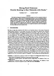
Table 2.1: A classification of real-time scheduling.
schedule is feasible. This scope is known as the task model of the system and conveys several of the factors discussed before, such as the criticality, attributes of tasks as well as their activation model. The existing scheduling approaches can be grouped into different classes according to ‘when’ the dispatching of tasks and the schedulability analysis are performed (see table 2.1). Dispatching means the decision process of choosing which task will run at each moment. Schedulability analysis is the process of determining whether or not the system is schedulable, i.e. timing feasible, for the assumed task model. In the off-line scheduling approach, cell (1) in the table, all tasks are scheduled off-line so that the dispatching time is determined in the design phase. The dispatcher just activates the tasks which are present in a scheduling timetable. This kind of scheduling is usually used in time-triggered systems [45]. The argument in favour of the off-line approach is its high level of predictability. Nevertheless, as has been observed [52], this is a questionable argument because the predictability is based on simple task models with strong timing assumptions, which makes the approach fragile and inflexible. In order to reduce this inflexibility, it is possible to perform some slight modification in the off-line generated schedules, preserving its timing guarantee, after it is derived off-line. This approach, represented in cell (3), is unusual but can be found in the literature [42]. The on-line scheduling approach, represented in cell (4) in the table, is so called because both the analysis and the dispatching are performed at run-time. Actually, the schedulability analysis becomes an acceptance test. The test checks whether or not, for each new arriving task, deadlines may be missed. If so, the task is rejected. Al-
2.3. The Scheduling Problem
35
though on-line schedulers represent the most flexible approach, they have quite poor performance in overload conditions [19] and cannot be completely predictable. Task rejections may mean missed deadlines. This approach can be used, for example, for scheduling soft/firm tasks. Most flexible scheduling schemes aimed at hard real-time systems lie in cell (2) in the table. The best accepted are those that are priority-based, where tasks are associated with priorities and the dispatcher chooses the highest priority task that is ready to execute. If the task priorities do not change at run-time, the scheduling approach is named static, or fixed priority. Otherwise, they are dynamic. Fixed-priority schemes assign priorities to tasks off-line. The priority assignment is usually based on task attributes such as period or deadline, classical examples being the Rate Monotonic (RM) [61] and Deadline Monotonic (DM) [5], respectively. In the case of the dynamic approach, priorities are determined on-line and reflect the urgency of execution. The Earlier Deadline First (EDF) [61] is an example of a dynamic approach, where the highest priority is given to the active task with the nearest deadline. Its disadvantage is the poor performance under overload conditions. Fixed-priority based schedulers, on the other hand, provide predictability [14, §13] and some approaches can cope with arbitrary deadlines. These characteristics may provide a trade-off between predictability and flexibility.
2.3.1
Fixed Priority Scheduling
In 1973, when the RM algorithm was published [61], the fixed priority scheduling theory started. The simple idea is to assign priorities to tasks so that the longer the period, the lower the priority. It assumed a strict task model, which may preclude the applicability of this approach. Indeed, this algorithm relies on a task model in which all tasks are periodic, independent and whose deadlines are equal to their periods. Later on, the applicability of the fixed priority scheduling was dramatically widened with the DM algorithm [40, 4]. The priority assignment is based on task deadlines instead of periods. The longer the deadline, the lower the priority. Its assumptions became weaker allowing arbitrary deadlines, sporadic tasks and task dependencies. As far as schedulability analysis is concerned, there are two main approaches used in fixed priority scheduling: utilisation bound and response time. The utilisation bound
2.3. The Scheduling Problem
36
of a task set is defined as the sum of the quotient between the worst-case computation time and the period of each task in the task set. Although simply defined, utilisationbound based analysis has some drawbacks. Firstly, it is only a sufficient analysis. In other words, the analysis finds an upper bound below which the task set is schedulable. After this bound nothing can be said in respect to the schedulability of the task set. Secondly, as for the rate monotonic algorithm, it presents a low level of processor utilisation: for a large number of tasks it is about 69% [61]. This means that large task sets with higher processor utilisation are considered unschedulable. By contrast, response time analysis is based on the derivation of the worst-case response time of each task in the task set. If, for any task, such a time is not greater than the task deadline, the task set is schedulable. The advantages of this approach are that: it can cope with arbitrary deadlines; it can support sporadic tasks; dependencies among tasks can be incorporated into the analysis; and when the analysis is applied to the same task model considered by the rate monotonic algorithm, it represents an exact analysis. This latter characteristic means that the analysis shows upper bounds on schedulability as well as lower bounds on non-schedulability. In other words, a task set is considered schedulable if and only if the analysis shows it is so [44]. When it comes to task dependencies, the problem of determining the maximum time that a task can be blocked has to be addressed. Blocking times are due to shared resources. For example, the following situation may happen in the context of fixedpriority scheduling. A lower priority task locks a resource that is used by a higher priority task. Then this higher priority task is released and will be blocked when it requests the already locked resource. This priority inversion may have worse consequences since a chain of blocking can lead to deadlocks. Traditional approaches based on breaking the chain to resolve deadlock conflicts [6] may be unacceptable in the context of real-time systems since it usually requires task cancellation. The widely used approach to solve this problem is provided by priority ceiling protocols [83]. The basic idea behind priority ceiling protocols is very simple and can be briefly explained as follows. Consider two fixed-priority scheduled tasks that share a resource. When the lower priority task is using the resource, its priority is raised so that if the higher priority task is released it cannot be selected by the dispatcher to execute. The lower priority task has its priority restored to the original level as soon as it stops using the shared resource. Then, the higher priority task can preempt the lower priority one.
2.4. Fault Tolerance
37
Although higher priority tasks may still be blocked by lower priority tasks (if they share the same resource), some characteristics make this protocol very interesting: • the blocking time due to lower priority tasks is minimised; • the worst-case blocking time is fixed and can be determined beforehand; • deadlock scenarios are avoided; and • as blocking conflicts are resolved by priority manipulation, management of explicit locks is not required. It is important to emphasise the flexibility provided by fixed-priority scheduling and response time analysis, where non-restrictive task models can be assumed. Dealing with dependencies among tasks through priority ceiling protocols exemplifies this flexibility clearly. Indeed, as described, these protocols work by changing the priorities of tasks at run time. In other words, the fixed-priority scheduling approach can, to some extent, deal with ‘dynamic’ priority assignments. The use of fixed-priority scheduling and response time analysis will be described in more detail in chapter 3.
2.4
Fault Tolerance
When something deviates from what was specified or intended, a failure happens, which is, in reality, an externalisation of an error (an incorrect internal state) [53]. The causes of both failures and errors are called faults. Defining faults and failures is important because one can analyse, based on the characteristics of the system/environment, how the system is more likely to fail. This analysis, in turn, helps in the definition of the right strategy that makes the system more reliable. Sections 2.4.1 and 2.4.2 present an introduction to some concepts about faults and failures, respectively. Four sort of techniques deal with faults: fault prevention, validation, fault forecasting and fault tolerance [53]. The former is intended to avoid occurrences of faults. However, it only minimises the number of them because, in general, faults are unavoidable. Validation is a complementary approach and its purpose is to avoid failure occurrences. It aims to reach confidence in the system’s ability to deliver a service complying with
2.4. Fault Tolerance
38
the specification [53]. Fault forecasting deals with the estimation of the present number, the future incidence and the consequences of faults. Fault tolerance, which is the focus of this thesis, assumes that faults are unavoidable and offers a set of techniques to tolerate them. The main approaches used to fault tolerance are summarised in section 2.4.3. Rather than describing specific implementation of these approaches, it presents an overview of available strategies that can be used to provide fault tolerance.
2.4.1
Faults
The structures of systems are inherently hierarchical, i.e. components are composed of other components and so on. Thus, a failure in one lower component can be seen as a fault by all higher components which use the lower one. This leads to the study of faults and their sources, which in general are extremely diverse. In order to prepare upper layer components to tolerate faults in lower ones, it is necessary to bear in mind the kind of faults the system is more likely to experience. For example, if the fault is permanent, an alternative component with similar functionality that provides a similar role in the system is necessary. Most design faults, whether in hardware or in software, are examples of permanent faults. On the other hand, if a fault is temporary it may be enough to re-request the services provided by this component after the error is detected. Temporary faults are those that are present in the system for a limited amount of time. They can be either transient or intermittent. The former originates from some disturbances in the external environment and the fault disappears after the disturbances cease. (e.g. electromagnetic sources may interfere in the behaviour of some system component). Intermittent faults result from the presence of rarely occurring combinations of conditions with respect to the internal state of systems. For example, temperature variation can cause changes in the parameters of a hardware device (e.g. memory, sensors etc). A more comprehensive classification of faults can be found in the literature [53].
2.4. Fault Tolerance
2.4.2
39
Failures
As indicated above, the correctness of a system is defined in both the value and time dimensions. A failure happens over the value dimension if the values produced do not comply with the given specification. Over the time dimension there can be the following kinds of failure: omission failures when the expected value is never produced; late failure when the expected value is produced too late; and early failure when the value is produced too early. Note that omission failure can be seen as a common limiting case for both value failure (null value) and timing failure (infinitely late). A persistent omission failure is called a crash failure. Omission failures belong to the stopping failure class: the system activity, if any, is no longer perceptible. The most generic kind of failure is called arbitrary or Byzantine, which involves all kinds of failure in value and time domains. Another sort of failure should be identified, called commission failure. This failure is characterised by having a service delivered when or where it is not expected [14, §5]. As a system is constituted of components that provide the system’s services, the utility of defining these type of failures is to bound the scope within which its components may fail. All the possibilities are represented in figure 2.2. For example, suppose that the components of a given system may fail only by omitting their expected services. This means that fault tolerance must be carried out aimed at tolerating the crash or omission of their components. The more generic the assumption on failures regarding a given system, the more robust the system is.
2.4.3
Approaches to Fault Tolerance
Intuitively, if any component of a system fails, whether it is hardware or software and however it fails, it is natural to think of redundant components being used to make the system deliver specification-compliant services. Therefore, choosing an approach to fault tolerance is, in fact, determining how redundancy is implemented. This choice, in turn, may depend on the system fault model. The fault model of a system is a set of assumptions on the kind of faults that are likely to be present (e.g. permanent or temporary) and how the system components may fail (e.g. omission or crash). The fault model must be the result of analysing the characteristics of the system/environment.
2.4. Fault Tolerance
40
Late Omission
Early
Crash Crash
Commission
Omission
Time Domain Value Domain
Null value
Arbitrary
Figure 2.2: Different kinds of failures and their relationships.
Once the system fault model is known, the approach to implementing redundancy in the system can be addressed. Although there are several different possible choices, one can group them by the kind of redundancy employed. Here, the system redundancy is classified according to two viewpoints: domain and behavioural. From the domain viewpoint, redundancy can be implemented in two non-exclusive ways: space and time. Space redundancy is employed by any extra hardware/software component that is introduced in the system just for fault tolerance purposes. For example, possible corrupted messages that are transmitted across a network can be detected by adding extra information to the message. One method widely used is based on the use of CRC (Cyclic Redundancy Checksum). By contrast, time redundancy is based on repeating the computation. For example, to make the system cope with message omission, the message must be required to be transmitted again. It is important to emphasise that redundancy in both domains, space and time, can be non-exclusively implemented. In the given example, the CRC (space redundancy) can be used together with message retransmission (time redundancy) to provide fault tolerance. According to the behavioural viewpoint, redundancy can be distinguished between active and passive. Active redundancy is when extra computational effort is spent to prevent the effects of possible errors, regardless of whether or not errors are detected. Passive redundancy, on the other hand, uses extra computational effort when some error is detected. This means that redundant components remain passive during normal
2.5. Distributed Systems
41
operation of the system. They are activated upon error-detection. One would have space-active redundancy, for instance, if in the above example the system had several senders per message. With this arrangement the system would tolerate faults of both communication and senders. Time-active redundancy is less common, but possible. For example, consider one message sender in the system, which always transmits each message twice so that possible faults as for one transmission operation are tolerated. This may make sense when the communication delays are very high (e.g. communication between a distant spacecraft and the Earth). Waiting for the error detection may be time consuming. Some points are worth noticing. Firstly, implementing passive redundancy requires an error-detection phase, which is not necessary when active redundancy is used. Thus, when compared with passive-redundancy based methods, active redundancy usually has shorter latency in providing an error-free service. However, it also presents high costs. Thus, for non-critical services active redundancy may not be cost-effective. Secondly, since error detection is carried out by extra components in the system, when using passive redundancy one is actually implementing, to some extent, space redundancy. As this error-detection component is an intrinsic part of the approach, errordetection components are not taken into account when classifying the approach as passive redundancy. Finally, passive and active redundancy may be non-exclusive approaches. For example, after an error is detected in some component, one may require that another alternative service should be provided. If this new service is critical, space redundancy may be needed.
2.5
Distributed Systems
A distributed system can be informally defined as a set of autonomous nodes (machines) that communicate with each other only by means of a communication network. The meaning of the word autonomous must be emphasised here. Being autonomous means that a node has its own set of machinery so that it can be used to implement any computing system without needing parts of other nodes. This autonomy is what distinguishes distributed systems from parallel machines, in which nodes are tightly coupled and have some degree of mutual functional dependency. Nodes do not share
2.5. Distributed Systems
42
memory and all communication is done by exchanging messages across the network. The degree of independence among the nodes of a distributed system offers a great potential to implement fault-tolerant systems. Indeed, active redundancy can be implemented using different nodes so that any fault in one node can be masked. However, this potential is often limited by the uncertainty of distributed computation, which is caused by: the possibility of having partial failures, i.e. either nodes or the network (or parts of it) can fail; and the fact that each node has its own view of the whole system, which does not represent the current system state. In other words, the same independence and redundancy that are intrinsically present in distributed systems and are so desired for fault tolerance are also the factors that limit the use of such kinds of system. The following simple example illustrates the complexity of using distributed systems. Two processes, pi and pj say, are co-operating throughout their computation. Suppose a moment during the execution of pi when it is waiting for a message from pj in order to take a decision in accordance with pj ’s computation. As process pi eventually has to make progress (i.e. it has to meet deadlines), it cannot wait forever (neither can pj ). Hence, there may be a moment at which pi has to make progress regardless of pj ’s message. If some fault prevents pj ’s message from being delivered to pi , pi may violate safety. Recall that pi must not take a decision that may clash with the computation of pj . If pj is crashed, though, pi is free to take its own decision. However, there are no means of pi knowing whether or not pj is crashed. It might be that the message sent by pj is just late or missed. In the above example, no assumption was made about the time the processes need either to finish their computations or to have their sent messages delivered. This kind of system is known to comply with the asynchronous distributed model of computation [62, §8]. If bounds on both processing speeds and message transmission delays can be derived (i.e. both processing and communication are synchronous), the computational model is called synchronous [62, §2]. If the synchronous model was assumed, the above example would have a straightforward solution. Indeed, pi could wait for the expected message until the maximum message delivery time. Notice that this time would be a function of the assumed bounds. If the message did not arrive by then, pi could conclude that pj is crashed and would carry out its computation regardless of pj .
2.6. Fault-Tolerant Real-Time Systems
43
It is important to emphasise that solutions that depend on assumed synchronism bounds might lead the system to violate safety when such bounds do not hold. This situation can be seen in the illustrative example given above. Should the message sent by pj be late, pi may take the wrong decision. In the context of real-time systems, assuming synchronous processing is reasonable because one can determine processing speed bounds before-hand (e.g. by using schedulability analysis, recall section 2.3). However, assuming synchronous communication is often a point of concern. Indeed, the communication network is a shared resource and can be subject to failures and overload conditions. Due to these characteristics and the fact that distributed processes can only use the network for exchanging information, it may not be possible for a process to determine the reasons that caused a message to be missed: sender or network failures. In other words, the communication network introduces extra uncertainty into the system. Therefore, one should think of the communication network as a critical part of a distributed system. In order to circumvent the impossibility of using the asynchronous model and avoid unsafe solutions based on the synchronous one, other models have been proposed. These will be summarised in the context of a specific distributed problem in section 2.7.
2.6
Fault-Tolerant Real-Time Systems
The implementation of any fault tolerance technique in a given real-time system has impacts on the system computation. Indeed, since time and/or space redundancy is necessary to make the system fault-tolerant, the extra computational efforts used for their implementation have to be taken into account due to timeliness requirements. The sections below summarise several solutions to this problem.
2.6.1
Supporting Passive-Redundancy Based Techniques
In order to carry out passive-redundancy based techniques, the detection of errors is needed. Most solutions presented in the literature use primary and alternative tasks [12, 34, 36, 54, 74]. Primary tasks represent the usual computation that needs to
2.6. Fault-Tolerant Real-Time Systems
44
be performed in error-free scenarios. Alternative tasks contain actions that must be executed when some error is detected. These actions can be used either to recover the system (i.e. put the system in a previous error-free state) or to compensate the system for the detected error. One of the main advantages of using alternative tasks is the degree of flexibility it provides. For example, if a task fails during its execution, it may be possible to perform specific actions through alternative tasks to deal with the detected error. The following scenarios give an indication of how flexible the system can be: • Some real-time systems are intrinsically resilient to some kinds of temporary fault, where just ignoring the error may suffice. For example, in reading a temperature sensor, missing some readings can be acceptable. Thus, it is worth waiting for another cycle of processing to try to complete the reading action. Obviously, if necessary, an alternative task can be released in this case to undo possible partial processing of the faulty task. • In other temporary-fault scenarios it may be worth re-executing the faulty task. This means that the alternative and primary tasks are the same. This option may be effective if it is known that the error is unlikely to occur again. • Depending on the characteristics of the system/environment, it may be possible and desirable to put the system in a safe state. An alternative task may be used for this purpose. Shutting down devices/machines, turning valves to a safe position (e.g. closing them) are examples of such actions. • One may require that another piece of code should be executed after the error. This alternative code would be able to provide a degraded but acceptable service. This kind of action may be desired for tolerating, for instance, design software faults.
By choosing an appropriate alternative task after the error is detected and analysed, the system is actually reconfiguring and adapting itself to the fault scenario. Also, it is important to notice that the implementation of alternative tasks can be carried out by using facilities provided by some programming languages [14] (e.g. exception handling). However attractive this approach is, most proposals found in the literature,
2.6. Fault-Tolerant Real-Time Systems
45
nevertheless, restrict the task model and/or the kind of actions alternative tasks can perform. This, in turn, reduces the applicability/effectiveness of the approach. For example, some of the approaches assume that only the re-execution of the faulty task can be used. In these cases, only time-passive redundancy is employed. Some approaches rely on distributed architectures. These can make use of two different task allocation policies, static and dynamic. Tasks are statically allocated if they are pre-assigned to nodes. The advantage of this approach is that it avoids high communication costs and complex scheduling decisions that are usually employed by dynamic allocation. Also, static allocation allows designers to carry out some optimisation techniques in order to minimise a given cost [84]. For example, by letting dependent tasks be allocated in the same node, one would minimise communication costs. By contrast, dynamic allocation requires decisions about where tasks can execute at run-time. This allows dynamic adjustment to the system (e.g. load balance) but is costly. Usually they are employed for supporting aperiodic tasks. Static allocation is preferred for hard periodic/sporadic tasks. Both allocation approaches have been used in the context of fault tolerance. However, since the major concern in this thesis is to provide static schedulability guarantees for critical systems, dynamic allocation is not considered here. Interested readers are referred to other works [33, 35, 63, 64]. In the following sections it is non-distributed and static-distributed solutions that are considered.
Non-Distributed Systems One of the first scheduling mechanisms for fault tolerance purposes was described by Liestman et al. [55]. This mechanism only deals with periodic tasks, whose periods have to be multiples of each other. Another restriction is that the execution times of alternative tasks have to be shorter than the execution times of their respective primaries. The approach presented by Ghosh et al. [36] limits the recovery of faulty tasks to re-executing them. Only transient faults can be tolerated (e.g. design faults are not considered). As it is based on the RM priority assignment policy, its disadvantages are inherited by this policy.
2.6. Fault-Tolerant Real-Time Systems
46
An interesting approach to tolerating transient faults which is independent of the schedulability analysis being used has been described by Ghosh et al. [34]. However, only the re-execution of faulty tasks as a means of fault tolerance is assumed. Recently, an EDF based scheduling approach, which takes the effects of transient faults into account, has been proposed [54]. Its basic idea is to simulate the EDF scheduler and to use slack time for executing task recoveries given a fault pattern. Fault patterns, which are the assumed maximum numbers of errors per task, must be known a priori. Task recoveries can be modelled as alternative tasks that are released after error-detection. Another EDF based scheduling approach for supporting fault-tolerant systems has been proposed by Caccamo et al. [16]. Their task model consists of instance skippable and fault-tolerant tasks. The former may allow the system to skip one instance once in a while. The latter is not skippable (i.e. all instances have to execute by their deadlines) and is composed of a primary and an alternative part. The primary part is scheduled on-line and provides high-quality service while the alternative one is scheduled off-line and provides acceptable services. The approach presented by Ramos-Thuel et al. [77] is based on the transient server concept. Its basic idea is to explore the spare capacity of the task set to determine the maximum server capacity at each priority level. A server is an a priori created task used to service aperiodic requests. In their approach such requests are the detection of errors. The spare capacity allocated to the server is used for on-line dispatching decisions in the case of error occurrences. Although this approach seems interesting since higher priority levels are used to execute alternative tasks, a reasonable way of determining the server periods has not been presented. A very flexible approach that makes use of fixed-priority scheduling and response time analysis has been proposed by Burns et al. [12] and Punnekkat [74]. No restriction on alternative tasks is assumed. This approach shows that response time analysis can be straightforwardly adapted to take the execution of alternative tasks into account. This characteristic makes this approach very effective. For example, by not restricting the type of redundancy alternative tasks represent, this approach can be used to make the system tolerant to software design faults or some kinds of temporary faults. This approach will be detailed in the next chapter.
2.6. Fault-Tolerant Real-Time Systems
47
Distributed Systems with Static Task Allocation Bertossi et al. [7] have proposed a scheduling approach to tolerating crash failures of nodes. Their idea is based on carrying out periodic checkpoints during the execution of the task on different nodes. If one node fails, the execution of the task can be resumed in another node from the last checkpoint. In other words, they use passive redundancy in the time and space domains. This approach, however, imposes several restrictions. The assumed task model does not allow dependency between tasks and task periods have to be equal to deadlines. Also, the checkpoints have to be carried out synchronously in different nodes, which may be costly since the context of a task has to be periodically multicast across the system. Finally, it is assumed that fault detection is timely and reliable. Kandasamy et al. [42] describe a recovery technique that tolerates transient faults in an off-line scheduled distributed system. It is based on taking advantage of task set spare capacity. The amount of spare capacity is distributed over a given period so that task faults can be handled. Although tasks are assumed to be preemptive and their precedence relations are taken into account, only periodic tasks, whose periods are equal to deadlines, are considered.
2.6.2
Supporting Active-Redundancy Based Techniques
As indicated earlier, active redundancy only in the time domain is not very common. This is because performing the same computation more than once regardless of the presence of errors is not applicable in most of the cases. Indeed, redundancy in time usually only makes sense after error-detection. On the other hand, active redundancy in the space domain is widely used to support critical systems. A natural way of implementing it is using distributed systems. This kind of architecture offers a high level of hardware redundancy so that the same computation can be performed independently in different nodes. Thus, even if the computation performed in a node fails (and this includes failures of the node itself), faults can be masked. Clearly, if identical replication is employed, i.e. using the same hardware and software in the replication, design faults may not be tolerated. Using some diversity in the implementation of active redundant systems, therefore, is desirable.
2.6. Fault-Tolerant Real-Time Systems
48
There are some approaches in the literature that implement active redundancy. Perhaps the most widely known technique is the state-machine approach, also called active replication [82]. This approach has no centralised control. Replicas process income requests and output the results of their computation. To be fault-tolerant, all replicas must receive and process the same sequence of requests; every non-faulty replica must receive every request; and the order of request processing must be the same for every non-faulty replica. Needless to say, in a distributed environment such properties are not easily ensured. It is important to note that the specification of the active replication mentioned above does not mention timeliness, necessary for real-time systems correctness. Krishna et al. [49] considered that timeliness is already guaranteed in fault-free scenarios. Then, they presented an algorithm to introduce fault tolerance in case some replicated task fails. However, they do not deal with keeping the consistency of replicated computation. Indeed, if active replicas run out of order, they may produce different results. Similarly, the approach presented by Bertossi et al. [8] only deals with finding feasible scheduling of replicated tasks. Moreover, their approach, based on RM, does not allow more than one replica per task. In fact, ensuring safety and timeliness in an active replicated system is not only guaranteeing schedulability. In the MAFT (Multicomputer architecture for fault tolerance) [43] both problems have been addressed, where active replication is implemented. The replicas are scheduled in synchronous slots. Tasks are scheduled according to known fixed priorities and cannot be preempted within a slot. These characteristics ensure the relative order of replicated processing. The result of their computation is chosen by carrying out distributed agreement after their processing. An alternative to active replication is semi-active replication. This approach, also known as leader-followers, has been carried out in the Delta-4 project [71]. The basic idea is to have just one replica, the leader, taking all major decisions. The other replicas follow the leader. Inter-replica coordination is needed in order to synchronise the leader and the followers. When the leader fails, some follower becomes the leader. Although more flexible, this approach has a drawback. Indeed, there is a window in time after a possible failure of the leader when the system may be vulnerable since there may be a situation in which the followers do not have current information about the leader’s decisions.
2.7. The Consensus Problem
49
If it is possible to synchronise the processing of replicated tasks so that the results of the non-faulty processing are output within a known bounded time from each other, fault tolerance can be ensured straightforwardly. For example, a bitwise comparison of the results suffices. This approach is known as replica determinism [69] and was carried out in the context of MARS (Maintainable real-time system), which is a time-triggered system [45, §14]. To guarantee the determinism of replicas, replicated processing outputs are ordered by using knowledge about task deadlines [69]. Input requests are assumed to be periodic and synchronised, a property ensured by the time-triggered approach. The problem with replica determinism is that it usually imposes too much restriction on the system processing capabilities. An extension of this approach that is slightly more flexible has been proposed [70]. In this case, the processing output ordering is done by the knowledge about task worst-case response times instead of deadlines. Whatever strategy of active space redundancy is used in a distributed system, it is costly, although necessary for critical systems. Also, one class of problems will always be present, distributed agreement. Indeed, replicated processing needs to agree on the order of the processing, and/or on the results they produce and so on. The next section pays special attention to one example of these problems, namely consensus.
2.7
The Consensus Problem
Distributed computation may diverge due to the intrinsic uncertainty of this kind of architecture. Indeed, as seen in section 2.5, distributed processes may lead the system to scenarios where safety is violated. This situation is also an impairment to implementing fault-tolerant systems. For example, replicated tasks may reach different results after performing their actions. One may send a signal saying that a given valve has to be closed while the other may do the opposite. Clearly, the system has to provide ways for preventing this erratic behaviour. To do so, the system must be able to reach agreement on distributed computations despite faults. There are several kinds of agreement problem [62]. The research presented here has concentrated on one, the consensus problem. This problem states that a group of distributed processes that propose their initial (possibly different) values has to agree, despite faults, on a single value. The special interest in this problem comes from the
2.7. The Consensus Problem
50
fact that consensus is known to be fundamental in fault-tolerant distributed systems. Indeed, it has been shown that solutions to the consensus problem can be used as a basic building block to solve other agreement problems [10, 37, 38, 81]. For example, a well known theoretical result states that solutions for consensus can be used to solve atomic broadcast [37], which is another equally important agreement problem for fault tolerance purposes. The consensus problem is usually specified in terms of the following properties: • Eventual Termination: Every correct process eventually decides some value. • Validity: If a process decides v, then v was proposed by some process. • Agreement: No two processes decide different values. Actually, this specification of consensus is known as uniform consensus [65], a stronger version of the consensus problem, which states that no process (correct or not) can violate the agreement property. As real-time systems need timeliness guarantees, it is often necessary to strengthen the termination property. Thus, the consensus problem specified in terms of bounded termination, validity and agreement properties is considered here to be the timed consensus problem: • Bounded Termination: Every correct process decides some value within a maximum known interval of time. Due to its importance, the consensus problem has been extensively studied for decades. Usually, solutions that ensure the bounded termination property are proposed in the synchronous model of computation. In this model the detection of faulty components can be reliable and timely. For example, if the absence of a component activity violates the assumed bounds, other components can conclude that such a component is faulty. This predictable behaviour is the reason why active redundancy in real-time systems is usually proposed for the synchronous model. However, as discussed in section 2.5, these assumptions on the system synchronism may impose some restrictions on the design of systems.
2.7. The Consensus Problem
51
The use of purely asynchronous systems to solve consensus is not possible. Indeed, in their seminal paper, Fisher et al. [30] showed the impossibility of having deterministic fault-tolerant solutions of consensus in asynchronous systems. They proved that in such a model of computation, even if there is only one process that may crash, consensus cannot be solved. This astonishing result has motivated many other researchers to find ways of circumventing it and/or finding out the boundaries for consensus feasibility. Dolev et al. [22] have defined four minimal cases in which consensus can be solved out of 32 different computational models. These models are defined by playing with five key parameters: processing (synchronous/asynchronous), communication (synchronous/asynchronous), message order (messages are delivered in the same order as they are sent/absence of order), transmission mechanism (broadcast/point-to-point) and receive and send operations (atomic/separate). Other semi-synchronous models of computation that allow the consensus problem to be solved have been proposed [21, 25, 28]. These models usually take into consideration the fact that synchronism may not hold completely at all times. In general, the strategy to solving consensus in these models is to prevent the protocol from making progress (do nothing) in the case of loss of synchrony in order to be safe (make no mistake). This approach, however, does not guarantee bounded termination. Indeed, in real-time systems doing nothing may mean a mistake (missing deadlines). In another seminal paper, Chandra et al. [17] have augmented the asynchronous model with the concept of failure detectors. Failure detectors are entities that give (possibly unreliable) information about process crashes. In their original work, message omission is not considered. Some other failure detectors have been proposed for environments subject to message omission failures [1, 23], but these approaches do not deal with the bounded termination property either. Some semi-synchronous models of computation have been proposed in the context of real-time systems, namely quasi-synchronous [88] and timely computing base [89] models. These models are based on special communication networks. They assume that the system is divided into two distinct parts, one synchronous and the other semisynchronous. The synchronous part is used to control and adjust the semi-synchronous one, in which complete synchronism may not hold at all times. This allows the system to negotiate, at run-time, an appropriate quality of service when the semi-synchronous part cannot deliver all its services on time. However, the synchronous part assumes
2.8. Summary
52
that transmitted messages and processes are always timely. Timed termination can only be guaranteed if consensus is implemented in the synchronous part. Whichever model is assumed, solving consensus requires extra computational effort, which involves the exchanging of messages across the communication network. An interesting theoretical result in this respect is the lower bound in terms of the number of steps of communication needed to solve consensus. It is known that in order to tolerate c process crashes, one needs at least c + 1 communication steps [62, §6]. In the synchronous model under certain favorable communication patterns, this bound can be improved by min(c� + 2, c + 1), where c� is the actual number of processes that crash [24, 26, 78]. It is important to emphasise, however, that the synchronous solution to the consensus problem relies on strict synchronism assumptions. Also, in practice, synchronous consensus protocols usually make use of a global time view, implemented by clock synchronisation protocols, e.g. [3, 29, 66, 67, 76], which also needs communication resources.
2.8
Summary
A guarantee of both safety and timeliness is essential to hard real-time systems. Timeliness is ensured by appropriate scheduling mechanisms while fault tolerance is needed to guarantee safety when faults are considered. Yet, scheduling and fault tolerance cannot be seen in isolation. Indeed, appropriate scheduling mechanisms have to be aware of the fault tolerance technique used in order to take its effects into account. In turn, fault tolerance implementation can use the timing knowledge provided by the scheduling approach used. As far as scheduling is concerned the fixed-priority based approaches together with response time analysis provide a trade-off between flexibility and predictability. These characteristics have allowed this approach to be used successfully for fault tolerance purposes in non-distributed systems. Passive-redundancy based techniques are usually more cost-effective since extra computational effort is only performed when errors are detected. Active redundancy, on the other hand, is usually more costly, although often necessary for critical applica-
2.8. Summary
53
tions. Indeed, this sort of technique uses a high level of redundancy so that faults can be masked, avoiding the need for error detection. The potential of using distributed systems for providing fault tolerance is enormous. Indeed, it is an ideal kind of architecture to implement active-redundancy based techniques since the system computation can be spread out across different (and independent) nodes. However, distribution also makes the design of fault-tolerant systems very complex. In the core of the complexity issue lie solutions to agreement problems, among which the consensus problem is a fundamental one. The focus of the following chapters is on the development of an overall framework for fault tolerance in hard real-time systems. This framework provides support for reliable, flexible and predictable real-time systems, where scheduling is addressed in conjunction with fault tolerance. The scheduling mechanisms developed are based on fixed-priority and response time analysis. The fault tolerance technique used implements both passive (by scheduling alternative tasks) and active redundancy (by performing consensus protocol) in a complementary way. The major characteristic of the proposed approach is that computational correctness is ensured but system flexibility is preserved.
3 Computational Model and Initial Concepts
This chapter describes the computational model and the notation that will be used in the next chapters. This description involves defining the assumed task and fault models, the structure of the computing system and its characteristics and behaviour. Defining the computational model is important. As an abstraction of the real system, it highlights the relevant characteristics of the system while hiding unnecessary details. As mentioned in the previous chapter, solutions for supporting fault-tolerant real-time systems are often restrictive in terms of the task and/or the fault models. This is because they favour predictability to the detriment of flexibility. Unlike these approaches, the computational model defined in this chapter aims to achieve a trade-off between flexibility and predictability. In order to do so, the following points were observed: • The task model must be as flexible as possible so that possible recovery and/or compensation actions due to error occurrences can be easily implemented. This can be achieved by releasing alternative tasks upon error detection (passive redundancy). • Approaches based on fixed-priority scheduling and response time analysis must be used so that: the system can cope with a flexible task model; off-line timeliness guarantees and on-line task dispatching can be provided. 55
3.1. The Computational Model
56
• Fixed-priority assignment policies must be adequate to the fault tolerance approach used. The intuition behind this requirement is that if an error interrupts a given task, the system may have a stricter timing constraint to comply with. For example, the possibility of executing alternative tasks at higher priority levels is desirable. Therefore, traditional priority assignment (e.g. DM or RM) may no longer be appropriate to deal with such cases. Non-traditional approaches must be investigated. • Since critical tasks may be present, the system must provide support for implementing active redundancy in a distributed architecture. This involves solutions to the consensus problem, as mentioned in the previous chapter.
The definition of the assumed computational model is given in section 3.1. This section also introduces necessary notation. Then, in sections 3.2 and 3.3, approaches to solving scheduling and consensus in the context of the assumed model are discussed. A brief review of related work and the points on which further research is needed are also presented in these sections.
3.1
The Computational Model
The computing system makes use of a distributed architecture, as illustrated in figure 3.1. The network is a real-time bus-based network, as explained later. The computation in a node is carried out by one process, which contains one or more tasks. Processes (and so their tasks) are statically allocated to the nodes. For the sake of notation, some simplifications regarding the allocation of processes and tasks are made. The set of m processes in the computing system is denoted as Π = {p1 , . . . , pm }. The processes are allocated to the m nodes so that there is only one process per node. Thus, the tasks that run in a given node are associated with the same process. Clearly, in practice one may have several processes allocated to the same node. However, this assumption is simply to allow a process to be a generalised reference to the tasks allocated in its node. Since the concepts and results presented hereafter do not depend on how many processes are allocated to each node, this assumption is not a restriction of the computational model.
3.1. The Computational Model
57
Nodes
p1 Γ
p2 Γ
pm
...
Γ
message exchange Communication Network
Figure 3.1: Illustration of the assumed architecture.
Γj = {τ1,j , . . . , τnj ,j } denotes the set of nj tasks that are associated with a given process pj . This notation can be simplified by dropping the process identifier j. For example, if one makes reference to two tasks allocated to different nodes, the identifiers of their processes can be used instead (since there is only one process per node). References to tasks that belong to the same node can be made using their own identifiers. Hence, the task set can be written as Γ = {τ1 , . . . , τn }, which means that references to any two tasks implicitly mean that they are allocated to the same node. It is important to emphasise that this simplification in the notation is not ambiguous and serves for the purposes of this work. As for the communications network, its level of reliability is always a point of concern. Overload or fault conditions may delay or prevent the delivery of messages, which may cause distributed computation to diverge, for instance (recall section 2.5). In this context, it is essential that the communication network presents a high level of reliability and predictability. An example of a communication network that fulfils these requirements is CAN (Controller Area Network). CAN was developed by BOSCH for automotive systems [9] but is also widely used for supporting other hard real-time systems, such as those in the automation industry. The reliability and predictability provided by CAN comes from its built-in error-detection and processing mechanisms, its priority-based message arbitration scheme and the fact that it complies with the event-triggered paradigm. Another important factor
3.1. The Computational Model
58
that contributes to the broad acceptance of CAN is that the schedulability analysis of communication can be carried out using response time analysis similarly to the way it is done with tasks [85, 86]. Due to these characteristics, CAN, the kind of network assumed in this work, favours the development of flexible hard real-time systems. The assumed model of computation is detailed in the following sections. Section 3.1.1 describes the task and fault models within the boundaries of a node. The communication network and the fault model of the inter-node computation is given in section 3.1.2. Those assumptions that represent the basics of the defined model will be given special emphasis in the description that follows. This is done by enumerating and labelling them and has the purpose of highlighting the main characteristics of the described computational model.
3.1.1
The Intra-Node Model
All tasks in the system are hard. In the absence of fault scenarios, primary tasks are scheduled by the system. If any error is detected, an appropriate alternative task is released so that it can recover/compensate the system from the error. Errors are detected at the task level and errors are assumed to be detected by the computing system. The kinds of fault with which the passive redundancy provided by alternative tasks can deal are those that can be treated at the task level (recall section 2.6.1). Consider, for instance, design faults. It may be possible to use techniques such as exception handling or recovery blocks to perform appropriate recovery/compensation actions [12]. In addition, one may consider some kinds of transient fault, where either the re-execution of the faulty task or the execution of some compensation action is effective. For example, suppose that transient faults in a sensor (or network) prevent an expected signal (or message) from being correctly received at a node of the computing system. This kind of scenario can easily be modelled by alternative tasks, which can be released to carry out a compensation action in the node. However, it is important to emphasise that some kinds of fault that cannot be treated at the task level are not tolerated by the use of passive redundancy implemented within nodes. For example, if a memory fault causes the value of one bit to be arbitrarily changed, the operating system may fail, leading the whole node to be compromised. Severe faults are those that cannot be
3.1. The Computational Model
59
treated at the task level. As for these kinds of fault, it is assumed that one uses space redundancy involving more than one node to carry out fault tolerance. Each primary task has one or more alternative tasks associated with it. Primary tasks are either periodic or sporadic. The period of primary task τi ∈ Γ is denoted Ti . The other attributes of τi are its deadline, Di (Di ≤ Ti ), its worst-case computation time, Ci and its release jitter, Ji (Ji ≥ 0). Among all alternative tasks that may be associated with τi , τ i is the one that has the biggest recovery cost, denoted as C i . Recovery costs are the worst-case computation times of the alternative tasks and represent the computational time spent to recover/compensate the primary tasks from errors, in the worst case. Alternative tasks, whenever released, have to finish by the deadline of their primary. Primary tasks, regardless of the node they are allocated, are scheduled according to some fixed-priority assignment algorithm. This algorithm attributes a distinct priority to each task τi ∈ Γ: n different priority levels (1, 2, . . . , n) are assumed, where 1 is the lowest priority one and n is the size of Γ. The alternative tasks of τi execute at priority levels higher than or equal to τi ’s priority. The priorities of τi and τ i are denoted pr(τi ) and pr(τ i ), respectively. When a primary task, say τi , and an alternative task, say τ j , are ready to execute at the same priority level, τ j is scheduled first. It is important to emphasise the reasons behind the assumption on the priorities of alternative tasks. After an error the system certainly has a shorter period of time to complete the execution of the recovery/compensation actions. Therefore, it may be advantageous to execute alternative tasks at a higher priority level. As τ i is the most costly alternative task that is associated with τi , τ i will be used as a representation of all alternative tasks of τi . For the sake of simplicity, the costs associated with any dispatching operation regarding either primary or alternative tasks are not represented. Actually, these costs are in practice easily incorporated into the values of Ci and C i , respectively. When an error interrupts the execution of a task and an alternative task is scheduled, other tasks may suffer the effects of its execution in the time domain. For example, the finishing time of lower priority tasks may be delayed as a consequence of the execution of this alternative task. Thus, there is fault propagation in the time domain, i.e. a fault
3.1. The Computational Model
60
in one task may cause a timing failure (missed deadlines) in another task. However, it is assumed that there is no fault propagation in the value domain. In other words, errors affect only the results produced by the faulty task. It is assumed that there is a minimum time between consecutive errors, namely TE . This means that in the worst case errors interrupt tasks at a rate of 1/TE . It is clear that in practice error arrival rate is not periodic. However, it has been shown that this assumption is useful for the derivation of schedulability analysis for fault tolerance purposes. Indeed, Burns et al. [13] have proved that if error arrivals are modelled by a Poison distribution (a usual and often realistic assumption), then the probability of failure during the lifetime of the system is proportional to TE (i.e. the smaller the value of TE that can be accommodated, the more fault resilient the system). The value of TE , as will be seen in chapters 4 and 5 is going to be used as a metric of fault resilience. The following assumptions summarise the characteristics of the intra-node model: Assumption 3.1.1 (non-severe faults). All errors caused by non-severe faults are detectable at the task level. The occurrences of such errors in different tasks are independent of each other. Assumption 3.1.2 (error-propagation). There is no error propagation in the value domain within nodes. Assumption 3.1.3 (minimum time between errors). There is a minimum time between two consecutive errors.
3.1.2
The Inter-Node Model
Errors caused by severe faults are dealt with by replicating tasks in different nodes. Only those processes that perform very critical tasks need to be replicated. These replicas are not necessarily identical. This means that different programming languages, algorithms or hardware may be used in their implementation. If there is no error during the execution of the replicas, they must produce the same results given that they process the same input data. However, due to some variations in the system the view of different replicas may diverge. Examples of such variations are differences in task release times, task preemption, worst-case computation times
3.1. The Computational Model
61
and the hardware of the nodes. Due to these factors, replicas may process different input data and so they may produce different results. From the point of view of each replica, all these results are, nevertheless, correct. Instead of imposing restrictions on the computational model to get replica determinism (recall section 2.5), the consistency of the system holds by carrying out a consensus protocol. That is, all correct replicas are able to choose one of the produced results. This protocol must conform with the characteristics of the processes and the communication network as well as the assumed fault model.
Processes and Nodes The use of alternative tasks, as explained in section 3.1.1, must suffice to ensure that tasks (replicated or not) produce correct results in the presence of non-severe faults. If the error is caused by a severe fault, though, it is assumed that the node in which such an error occurs enters a silent state, where it stays indefinitely. If a node is in a silent state, the process allocated to it (and so its tasks) is also in a silent state. In other words, processes may only fail by crashing and crashed processes do not recover. This is usually known as the fail-silent assumption [53]. It is important to emphasise that the fault model regarding the processes and nodes can be implemented by employing special routines to shut down the node in the presence of errors caused by severe faults. Clearly, in this case there is an implicit assumption that such errors are detectable so that after an error, one may use special guards to prevent the node from transmitting further messages. For example, the message sending operation can be modelled as a task that is triggered by signals sent by the upper layers. If the operating system is down or malfunctioning, say, this task stops sending messages so that no invalid messages are sent. The fail-silent assumption has been used in other distributed real-time systems (e.g. [47]).
The Communication Network This section describes the general characteristics of CAN. Based on these characteristics the assumed fault model for communication is then presented. Rather than describing
3.1. The Computational Model
62
details of CAN, only relevant points, which are necessary to the definition of the assumed computational model, are addressed. The reader interested in more details of CAN is referred to specialised publications [9, 39]. Two main factors make CAN an interesting network for real-time systems: the deterministic priority-based bus arbitration and the way transmission errors are handled. The bus arbitration in CAN is a bit-wise protocol. Either a dominant or a recessive bit can be transmitted at a time on the CAN bus. If two nodes simultaneously transmit two different bits, the resulting bus value will be the dominant one. While a message is being transmitted, both the sender and receivers monitor the bus. Also, each message has a unique identifier (priority). Similar to the priority of tasks, pr(m) denotes the priority a message m. If pr(m) > pr(m� ), then message m has higher priority than m� . By having these characteristics, bus access conflicts are deterministically resolved by the following arbitration scheme. While transmitting the message identifier, for every bit, if the transmitted bit is recessive and a dominant value is monitored, the sender stops transmitting and starts receiving incoming data. Should a sender stop transmitting a message due to this arbitration scheme, its message is automatically scheduled for retransmission. This policy, known as carrier sense multi-access with deterministic collision resolution (CSMA/DCR), provides a predictable message scheduling mechanism for supporting hard real-time systems. Nevertheless, this bit-by-bit arbitration scheme also has some side-effects. The low network bandwidth is one of them. Indeed, the maximum transmission rate is 1 Mbps. The set of mechanisms that CAN provides to handle transmission errors is based on the passive-redundancy approach. Recovery is carried out by the automatic message retransmission (through the arbitration protocol) after transmission errors are detected. In brief, these mechanisms work as follows. If the sender does not detect errors up to the last bit of the end of the message, the transmission is considered successful and no retransmission is carried out. However, if the sender or some receiver detects some transmission error, it starts transmitting a stream of dominant bits so that the standard bit pattern on the bus is violated. This violation, known as the error flag, means that the message was not properly received at some node. When detecting either the error or the error flag, the other nodes start transmitting their error flags as well. Then, the nodes synchronise themselves by sending recessive bits and monitoring the bus.
3.1. The Computational Model
63
After synchronisation, nodes start transmitting their messages according to the bus arbitration scheme. This includes those messages that could not be transmitted in the first place due to errors.
Inconsistent Scenarios Although the error detection and recovery approach used in CAN can handle most transmission errors consistently, some inconsistency may still be present. In fact, it has been shown that in some scenarios a set of receivers can accept the message while others reject it [73, 80]. This can happen when the error is detected just at the last bit of the message by some nodes. The nodes that do not detect the error, accept the message while the others reject it. In this situation three inconsistent scenarios may take place: IS1 Inconsistent message omission due to crash failures. If the sender crashes after the detection of the error and before the retransmission, its transmitted message will be inconsistently omitted at some nodes. IS2 Inconsistent message duplication. If the sender does not crash, it retransmits the message and so some receivers may receive the message more than once. IS3 Inconsistent message omission due to undetected transmission error. The third scenario has the same effect as IS1 and happens if the sender does not crash but it does not detect the faulty transmission. Indeed, it may not detect the error flag if another error, which changes the last bit of the message to recessive, takes place at the sender node. Notice that the inconsistency caused by IS1 is associated with process crashes. Thus, both events have to happen, the error in the last but one bit and the crashing of the sender node. On the other hand, the errors that lead to IS2 or IS3 are related to the transmission of the message. The probabilities of occurrence for these inconsistent scenarios have been calculated [73, 80]. In one hour of transmission with 90% of workload these probabilities vary between 8.80×10⁻³ and 3.96×10⁻⁸ . It is important to emphasise that IS3 was first noticed by Proenza et al. [73], who have demonstrated that IS3 is 10 to 1000 times more likely to take place when compared with IS1. Although
3.1. The Computational Model
64
unlikely, all these three kinds of scenario have to be considered when dealing with critical applications. Indeed, as has been pointed out [72, 80], the aerospace industry recommends values not higher than 10−9 incidents per hour. Despite the possibility of inconsistent scenarios, the communication network is assumed to be non-partionable. This means that messages may be arbitrarily delayed or even dropped due to inconsistent scenarios, but non-crashed processes cannot be permanently disconnected from each other. For example, a lower priority message may suffer delay due to the retransmissions of higher priority messages. However, if there is no inconsistent scenario, this lower priority message is guaranteed to arrive at its destinations within a finite time. This finite time includes re-transmissions of messages in case of errors. Note that this assumption is in line with the characteristics of CAN since messages are automatically rescheduled for retransmission and errors are consistently detected apart from the inconsistent scenarios. Further, it is assumed that messages cannot be either arbitrarily created or corrupted by the network. Again, this is ensured by the reliability level provided by the CAN protocol. In cases where no inconsistent scenario takes place, it is correct to say that CAN provides atomic broadcast. In general, atomic broadcast states that: all messages transmitted by correct processes are eventually delivered at all correct processes (eventual delivery); if a message is delivered by a correct process, then the message is delivered to all correct processes (reliable broadcast); and all correct processes deliver messages in the same order (total order); and every delivered messages was sent by some process (integrity). It is not difficult to see that CAN provides eventual delivery and integrity but does not guarantee reliable broadcast or atomicity in the presence of inconsistent scenarios. As a summary of this section, the following assumptions can be highlighted. Most of these assumptions are associated with the characteristics of CAN. Assumption 3.1.4 (Severe faults). Severe faults may make the processes fail only by crashing. Crashed processes do not recover. Assumption 3.1.5 (Message ordering). Messages are assumed to have priorities and are scheduled for transmission according to their priorities. Assumption 3.1.6 (Network integrity). Messages are neither arbitrarily created nor corrupted by the communication network but they may be lost (by inconsistent
3.2. Response Time Analysis for Fault Tolerance
65
scenarios) or arbitrarily delayed (by the arbitration scheme of CAN). Assumption 3.1.7 (Eventual delivery). If a correct process broadcasts a message, then the message is eventually delivered to some correct process. Assumption 3.1.8 (Best-effort broadcast). If a message is delivered to a correct process and does not suffer inconsistent omission, then the message is delivered to all correct processes. Assumption 3.1.9 (Best-effort atomicity). Transmitted messages that do not suffer inconsistent omission/duplication are either delivered to all correct processes in the same order or they are not delivered at all. In order to make the computational model complete, the assumed level of timing synchronism, on both processing and communication, needs to be specified. A timing synchronism assumption usually made for real-time systems relates to the presence of synchronised clocks. This assumption can be guaranteed in the synchronous model of computation [3, 66, 76, 79, 90] while in some semi-synchronous models the system may suffer loss of clock synchrony [18, 20]. In this thesis, clock synchronisation is not assumed. This means that the solutions presented in the thesis will work properly regardless of the presence of synchronised clocks. The presentation of timing synchronism present in the assumed system is postponed to chapters 6 and 7. This is because these two chapters explore different sorts of synchronism in the system.
3.2
Response Time Analysis for Fault Tolerance
As mentioned in section 3.1.1, the effects of faults may propagate in the time domain since the execution of alternative tasks delays the finishing time of lower priority tasks. The focus of this section in on both determining whether or not these delays may cause deadlines to be missed and in which fault conditions the task set is schedulable. With this in view, response time analysis is used. The following sections present a brief introduction to response time analysis. Firstly, only fault-free scenarios are considered (section 3.2.1). Then, non-severe faults are
3.2. Response Time Analysis for Fault Tolerance
66
taken into account (section 3.2.2). Finally, in section 3.2.3, the main limitations of the current approaches are described. This description is illustrated by a simple example and represents one of the motivations for the research contained in this thesis.
3.2.1
Response Time Analysis in Fault-Free Scenarios
The use of response time analysis to derive the schedulability of task sets has been well accepted in the research community. Recalling section 2.3.1, its main advantages are due to the fact that off-line schedulability guarantees can be derived without impairing flexibility provided by on-line dispatching and non-restrictive task models. The basic idea is to derive the worst-case response time of each task in the task set. Once these values have been derived, a simple comparison with the task deadlines determines the schedulability of the task set. For any task τi ∈ Γ, its worst-case response time takes place when: all other higher priority tasks are released at the same time as τi ; and the execution of τi and all higher priority tasks τj take Ci and Cj to complete, respectively. In this scenario, the worst-case response time of τi , denoted Ri , can be written as [5]: � � Ri + Jj � Ri = Bi + Ci + Cj , Tj
(3.1)
j∈hp(i)
where Bi is is the worst-case blocking time of τi and hp(i) = {τj ∈ Γ| pr(τj ) > pr(τi )}. The operation �x� returns the smallest integer that is greater than or equal to x. Thus, �
Ri +Jj � Tj
gives the maximum number of releases of τj during the period Ri considering
possible release jitter effects. The value of Bi is fixed and can be deterministically computed due to the use of priority ceiling protocols [14, §13]. This value represents the maximum time during which τi may be blocked by lower priority tasks due to the use of shared resources (recall section 2.3.1). Since the term Ri appears in both sides of equation (3.1), it is solved iteratively applying the relation given by equation (3.2) [5]. The iteration can start with ri0 = Ci , where rik is the k th approximation to the true value of Ri . The interactions can be halted when rik+1 > Di or earlier if rik+1 = rik . In the former case, the task is not schedulable, while the latter means that Ri = rik . Yet, if the task suffers release jitter, the final value of
3.2. Response Time Analysis for Fault Tolerance
67
Ri is given by rk + Ji . rin+1
� � r n + Jj � i Cj = Bi + Ci + Tj
(3.2)
j∈hp(i)
In equations (3.1) and (3.2) multiple instances of the same task are not being considered. This is because, by the assumed task model, task deadlines are not greater than task periods.
3.2.2
Response Time Analysis in Fault Scenarios
As mentioned in section 2.6.1, response time analysis has been extended to take into account the execution of alternative tasks [12, 74]. The primary and their respective alternative tasks are assumed to run at the same priority level. Also, their approach relies on assumption 3.1.3. In order to understand the use of response time analysis in the context of fault tolerance, initially consider that only one error may take place during the execution of τi . Any task that may be executing concurrently with τi (including τi itself) may be interrupted by this error. In the worst-case scenario, the error interrupts tasks just before the end of their execution and the faulty task is the one with the longest recovery time among τi and all tasks that may preempt the execution of τi (i.e. tasks in hpe(i) = {τj ∈ Γ| pr(τj ) ≥ pr(τi )}). Assume that τk is such a task. This means that the time to recover τk (i.e. C k ) has to be added to the response time of τi . These observations lead to equation (3.3). Since Ri appears on both sides of the equation, its solution is obtained iteratively by forming a recurrence relation similarly to equation (3.1). For the sake of simplicity, release jitter and blocking effects are not being considered in this equation, although they can be easily be incorporated into the analysis. � � Ri � Ri = Ci + Cj + max C k , τk ∈hpe(i) Tj
(3.3)
τj ∈hp(i)
Nevertheless, errors may interrupt the execution of τk more than once. As in the worst case, errors interrupt tasks at each TE time units, the maximum number of errors that may take place during the execution of τi is given by � RiT(TEE ) �. This leads to equation
3.2. Response Time Analysis for Fault Tolerance
Task set Task Ti Ci C i τ1 13 2 2 25 3 3 τ2 30 5 5 τ3
Di 13 25 30
pr(τi ) 3 2 1
68
TE = 11 Ri 4 8 22
Table 3.1: A task set and the derived worst-case response times.
(3.4). As TE is an input to the analysis, Ri is now given as a function of TE , i.e. Ri (TE ): � � � � Ri (TE ) � Ri (TE ) Ri (TE ) = Ci + Cj + max C k τk ∈hpe(i) Tj TE
(3.4)
τj ∈hp(i)
It is interesting to note that equation (3.4) is conservative in the sense that in practice some of the errors may not interrupt the task with the longest recovery cost. Assuming that errors always interrupt the execution of such a task, however, simplifies computation. As an illustration, consider a set of 3 tasks and their alternative tasks shown in table 3.1. The values in the last column of the table are the worst-case response times for TE = 11. To illustrate this, the following is what the iterative computation of R3 (11) looks like: r30 (11) = 5 r31 (11)
=
r32 (11) = r33 (11) = R3 (11) =
3.2.3
�
� 5 5+2+3+ 5 = 15 11 � � 15 5 = 22 5+2+2+3+ 11 � � 22 5 = 22 5+2+2+3+ 11 22
On the Priorities of Alternative Tasks
As far as fixed-priority based scheduling is concerned, the worst-case scenario for the tasks is usually characterised by the time at which all tasks are released at once. This is assumed when either RM or DM assignment algorithms are used, for instance.
3.2. Response Time Analysis for Fault Tolerance
69
pr(τj ) (a)
pr(τi ) = pr(τ i ) Dj
Di
Dj time
pr(τ i ) pr(τj )
(b)
pr(τi ) Dj τ
τ
Dj time
Di Error
Preemption
Figure 3.2: Priority assignment in fault-scenarios: (a) primary and alternative tasks execute at the same priority level; (b) a non-traditional priority assignment as for alternative tasks is considered.
Under this scenario, it can be shown that these algorithms are optimal [14, §13] in the sense that if a task set is schedulable with a given priority assignment, then it is also schedulable with the priorities assigned by the RM or DM. When alternative tasks are considered, this optimality may not hold. In fact, the priorities of alternative tasks may follow different reasoning. The intuition behind this observation is that, after an error, tasks (or their recovery/compensation actions) certainly have a shorter period of time to meet their deadlines. Consider figure 3.2, where the execution time line of two tasks, {τi , τj }, is shown. The priorities of τj and τi follows the DM approach, i.e. pr(τj ) > pr(τi ), since Dj < Di . Associated with τi is its alternative task, τ i . An error interrupts τi just before the end of its execution, as illustrated. In scenario (a), it is assumed that τ i is executed with priority level pr(τi ) whereas in scenario (b) the priority of τ i is greater than the priority of τj . As can be seen from the figure, in (a) τi is not schedulable due to the preemption caused by the execution of the second release of τj . This preemption is avoided by executing τ i at a higher priority level, as illustrated in scenario (b). Response time analysis has been used in the context of fault tolerance, as explained in section 3.2.2. However, this has been done under the assumption that the priority of primary and alternative tasks are the same. This approach may introduce extra
3.3. Consensus in CAN
70
pessimism, as illustrated in figure 3.2. Indeed, the search for non-traditional approaches to finding out optimal priority assignments for alternative tasks is necessary. If traditional priority assignments are no longer appropriate when dealing with alternative tasks, neither is schedulability analysis that relies on them. For example, it can be seen from figure 3.2 that the response time of a task is determined not only by the execution of higher priority tasks but also by the execution of the alternative tasks of lower priority ones. Moreover, the worst-case scenario may not be simply characterised by the instant at which all tasks are released at once. This latter observation can be seen from the figure, where the worst-case response time of τj is when it is released just after τi is interrupted by an error. In summary, in order to use a response time based analysis that takes into account the effect of non-severe faults in nodes of the system, one needs both non-standard priority assignment approaches and to adapt the schedulability analysis to cope with these assignments. New results in this area are presented in chapters 4 and 5.
3.3
Consensus in CAN
The fact that inconsistent scenarios may take place is a limitation in solving consensus in CAN. This is better explained in section 3.3.1. Indeed, apart from these scenarios CAN provides what is know as atomic broadcast, as briefly mentioned in section 3.1.1. Like consensus, atomic broadcast is another agreement problem [37]. This problem states that processes atomically deliver the same set of messages and in the same order. A message is atomically delivered if it is delivered by all processes or by none. If CAN provided atomic broadcast, consensus would be trivially solved. For example, the following protocol would suffice: processes atomically broadcast the values on which they need to agree; and each correct process picks up the value contained in the first delivered message. Since messages are totally ordered and atomically delivered, all correct processes pick up the same message and so they reach an agreement on the value such a message contains. Although the problem of consensus alone has not yet been addressed in CAN, there have been some proposals to make CAN provide atomic broadcast. As consensus and
3.3. Consensus in CAN
p1 p2 p3
p1 p2 p3
71
a
a, c, a, b
b
a, c, a, b
c
c, a, b
a
a, c, b
b
a, c, b
c
c, b
(a)
(b)
Figure 3.3: Inconsistent scenarios as an impairment of consensus.
atomic broadcast are closely related problems [37] (i.e. one can be used to solve the other), these studies are briefly surveyed in this section. They are divided into softwarebased (section 3.3.2) and hardware-based solutions (section 3.3.3). While the former use standard CAN and build the solution in upper layers, the latter change the basic CAN protocol at the hardware level.
3.3.1
The Consequences of the Inconsistent Scenarios
Consider three processes, p1 , p2 and p3 that are executing tasks which need to reach consensus on the results of their computation. Let these results be a, b and c, respectively. See figure 3.3 as illustration, where the horizontal and diagonal lines represent the time arrow and message broadcast, respectively. If a diagonal line end in an arrow, the reception of the message is successful. Otherwise, a transmission error occurs. In the figure, the processes send messages to each other in order to exchange information and proceed with the necessary agreement. As can be seen, two inconsistent scenarios are illustrated. In (a) an inconsistent duplication takes place while in (b) a message
3.3. Consensus in CAN
72
is inconsistently omitted. In both scenarios there are no means for the processes to choose a single value. In (a), although all processes receive all the values, processes p1 and p2 receive a twice. In other words, messages are being delivered out of order at different nodes. Thus, processes cannot use a common criterion such as message order to choose one of the received values. It can be noticed that no other criteria may be used since there is not enough information at the processes. Indeed, from the point of view of each individual process, they do not know what messages were remotely delivered. For example, from the point of view of p2 and p3 scenarios (a) and (b) are the same. However, they cannot choose value a in (b) since p3 does not receive it. This problem seems to be even worse. Even if no inconsistent scenarios had happened, the processes could not have chosen a common value either. Indeed, they would not have known whether or not the inconsistent scenarios have taken place. In other words, a more elaborated protocol, which certainly involves more communication effort, is necessary to circumvent the difficulties due to the inconsistent scenarios.
3.3.2
Software-Based Solutions
The first solution for atomic broadcast in CAN was proposed by Rufino et al. [80]. Their approach is based on the following protocol, named TOTCAN (Totally ordered broadcast protocol). Sender processes request the CAN layer to transmit the application messages. The receiver processes that receive these messages store them in a buffer and wait until they receive an accept message. There is an accept message associated with each application message. If an accept message is not received by a pre-defined time after the application message was received, it is assumed that its sender process is crashed. In this case, the corresponding application message is discarded by the receivers in order to avoid IS1 (IS3 is not considered). If the accept message is received, though, the receivers remove the corresponding application message from the buffer and deliver it to the application. Duplicate messages, if received, are discarded. TOTCAN ensures atomic broadcast by relying on the the fact that the accept message does not suffer inconsistent omission. This assumption is guaranteed by another broadcast protocol, called EDCAN (Eager message diffusion on CAN). EDCAN is a non-ordered but reliable broadcast protocol and works by making each receiver retransmit the received accept message. Inconsistent message duplication may take place but this does not affect the behaviour of TOTCAN. Since accept messages do not need to contain
3.3. Consensus in CAN
73
application data, the implementation of EDCAN can be optimised (for details refer to Rufino et al. [80]). This diffusion-based solution is considered costly since bandwidth is a limited resource in CAN. The approach proposed by Pinho et al. [68] relies on the assumption that nodes have synchronised clocks, which can be implemented by specific protocols [90, 66, 79]. Whenever a process sends an application message, it also sends a confirmation message. The receivers store the received application message in a buffer and wait for predefined timeouts associated with each application message. There are two timeouts. The first is the maximum time during which the receivers must be waiting for the confirmation message after receiving the application message. The second marks the time at which the receivers must deliver the application message. Since the clocks are assumed to be synchronised, messages are delivered approximately at the same time. The timeouts are set upon the receipt of the application message. Should IS1 or IS3 occur and some receiver has not received the application/confirmation message, it sends an abort message so that all nodes can discard the associated application message. This abort message must arrive at all nodes before the second timeout expires, otherwise, some receivers may discard the message while others deliver it. Possible message duplicates are discarded by the receivers but the timeout values are updated accordingly. This makes the approach resistant to IS2 as well. This protocol, like TOTCAN, may not be completely reliable since some transmitted messages may never be delivered due to abortions. This problem can be avoided by carrying out a message diffusion, like EDCAN, which may be costly. Also, it is important to emphasise that the possibility of two inconsistent scenarios happening regarding the transmission of the application and its confirmation message is considered negligible and so not taken into consideration by the proposed protocol. Both solutions described in this section only work in the synchronous model of computation. Recall that synchronous systems are those where it is possible to determine bounds on message transmission and processing speeds. The solution offered by Rufino et al. [80] does not need clock synchronisation. Also, it is safer regarding possible loss of synchronism: if the assumed synchronism does not hold, messages are discarded but are not delivered out of order, a property that does not hold for the solution by Pinho et al. [68]. However, TOTCAN does not tolerate IS3.
3.3. Consensus in CAN
3.3.3
74
Hardware-Based Solutions
A hardware-based solution has been proposed by Kaiser et al. [41]. First, they solve the problem caused by IS1 (IS3 is not considered). This is ensured by special nodes plugged into the network, called SHARE (Shadow re-transmitters). The role of SHARE nodes is to start message retransmission after some message transmission error regarding the last but one bit of the message is detected. SHARE nodes start retransmitting the message regardless of original sender status (crashed or not), which means that a possible crash of the sender is masked. Once it is guaranteed that all messages are reliably delivered, atomic broadcast is carried out. This, in turn, is done by making use of knowledge about message deadlines and it is assumed the message scheduling is analysed and dispatched off-line. Therefore, this solution uses application-level information and is not flexible due to the message scheduling approach used. The approach proposed by Proenza et al. [73] has addressed the problem of atomic broadcast taking into consideration the three inconsistent scenarios. They have observed that whenever an error is detected, the CAN hardware provides internal information which indicates whether or not the node is the first to detect the error. This internal information can be used to handle errors in the last but one bit of the message. Errors in other bits are treated by the standard CAN protocol. The proposed modification in the hardware layer is very simple. In cases of potential inconsistent scenarios (errors in the last but one bit of the message) the node checks the internal information about primary error. If the node is not the first to detect the error, it rejects the message (if it is a receiver) or retransmit it (if it is a sender). Should the node be the first to detect the error, the message is accepted/not retransmitted. This rule works because whenever the node is the first to detect the error, the other nodes have already accepted the message. Therefore, implementing this rule at the hardware level, one avoids scenarios IS1 and IS2. This simple and efficient protocol is named MinorCAN. However, MinorCAN cannot cope with scenario IS3 since it is characterised by the fact that the sender does not detect the error. An additional modification of the basic CAN protocol, called MajorCAN [73], is needed. MajorCAN uses the approach described for MinorCAN to deal with scenarios IS1 and IS2. As for IS3, MajorCAN uses an extended error flag so that it can cope with successive corrupted bits in the end of the message. The number of bits in this flag is
3.4. Summary
75
a function of the number of expected errors. Making use of this new flag and assuming that the occurrence of more than k successive errors in the end of the message is unlikely, the problem of non-detected transmission errors at the sender node can be solved. Recall that IS3 is only possible because there are in fact two errors in the last bit of the message. One is at some receiver node(s), which makes the receiver(s) reject the message. The other is at the sender node, which prevents the message from being retransmitted.
A Required Solution Although computationally more efficient, hardware-based solutions are costly due to the required modifications of the standard and widely used CAN protocol. This observation has driven the research presented in this thesis to look at software-based alternatives that deal with the consensus problem, where flexibility and cost-effectiveness can be achieved without impairing predictability. There is a considerable number of generic solutions for the consensus problem (e.g. refer to [37, 62]). Some of these solutions could be used in the proposed model of computation. However, since they are generic, they do not use the particularities of CAN. Therefore, they are usually too costly to be employed for a low-bandwidth network such as CAN. As seen in this chapter, CAN offers an attractive set of properties. Taking advantages of these properties to design a flexible and efficient consensus protocol is one of the goals of the thesis.
3.4
Summary
A computational model for fault-tolerant real-time systems has been presented. The computing system follows a CAN-based distributed architecture. Fault-tolerance in each node is carried out by scheduling alternative tasks to perform necessary recovery/compensation actions and a flexible task model is assumed. This allows the system to be adjusted to fault scenarios since alternative tasks can be modelled based on the knowledge of the system/environment.
3.4. Summary
76
The scheduling of alternative tasks in each node follows the fixed-priority approach, where response time analysis can be effective in providing off-line timeliness guarantees. However, traditional priority assignments may lead the system to be too conservative regarding fault tolerance. Thus, other (non-traditional) priority assignment algorithms are desired. These algorithms have to take into consideration the scheduling of alternative tasks so that the fault resilience of the system is improved. In turn, response time analysis also needs to be adapted in order to be able to cope with such non-traditional priority assignments. Further research on both problems, schedulability analysis and priority assignment for fault tolerance purposes, is needed. Indeed, response time analysis has only been addressed by the research community using traditional priority assignment. Severe faults may prevent alternative tasks from being scheduled. Therefore, critical tasks must be replicated in two or more nodes of the computing system. The consistency of replicated computation is ensured by performing a consensus protocol which prevents distributed computation from diverging. Although the assumed communication network is very reliable, it presents some inconsistency in some specific scenarios. Unfortunately, proposed solutions to this problem either do not consider all possible inconsistent scenarios or are inflexible ones. Thus, the problem of consensus for CAN networks must be further investigated. In the next chapters solutions to the problems of scheduling using response time analysis, non-traditional priority assignments and software-based consensus for CAN will be addressed. The focus of these solutions is on flexibility, cost-effectiveness and predictability.
4 Response Time Analysis for Fault Tolerance Purposes
As seen in the previous chapters, fixed-priority scheduling and response time analysis have successfully been used for taking into account the execution of alternative tasks that carry out fault tolerance. Also, it is desirable that some alternative tasks have higher priorities than their respective primary tasks. The intuition is that alternative tasks may finish earlier if they execute at higher priority levels, which may make the task set able to cope with further errors without impairing its schedulability. Unfortunately, if a more flexible priority assignment is assumed as for alternative tasks, the schedulability of the task set cannot be derived by the usual analysis. Deriving schedulability analysis that takes non-traditional priority assignments into consideration is the subject of this chapter. The complexity of deriving response time analysis that takes into account alternative tasks running at higher priority levels (given by some non-traditional priority assignment policy) should not be neglected. Firstly, worst-case scenarios need to be characterised. Then, the analysis has to be developed to reflect such a characterisation. The characterisation of worst-case scenarios includes several factors such as the recovery times of the tasks, the priority at which alternative tasks are executed and the time the error takes place. For example, consider a task τi ∈ Γ and the following scenarios,
77
78
where an error interrupts: (a) a task that executes with priority higher than the priority of τi ; (b) a task with lower priority than the priority of τi but its alternative task may interfere in the execution of τi ; (c) τi itself. Also, note that there might be a combination of these scenarios, where more than one error takes place. For example, a scenario (d) would be: an error may hit a lower priority task, then another error hits τi and others may interrupt the execution of higher priority tasks. The characterisation of worst-case scenarios developed in this chapter follows a divideand-conquer strategy, where it is assumed for each task τi in the task set that: either errors interrupt the execution of tasks other than τi ; or τi may be faulty. The analysis is then derived accordingly, where the two branches of equations associated with this characterisation are developed (with or without errors in τi ). Splitting the computation into these two branches simplifies the derivation of the analysis since it turned out that if τi is not faulty, the worst-case is when the faulty task is the one with maximum recovery time. Once the values given by both branches of the computation are known, they can be used to derive the worst-case response time of τi . When errors in τi take place, both the characterisation of the worst case and the derivation of the analysis get more complicated. This is due to the fact that if τ i executes at higher priority level, two levels of priorities have to be considered, before and after the error. The worst-case response time of τi (together with τ i ) is now given by the time necessary to execute both τi and at least one release of τ i plus all higher priority tasks that may interfere in their execution. However, the set of tasks that may be released during the execution of τi and τ i may vary. This fact in isolation may not be a problem but other complications have to be addressed. Indeed, as response time analysis is an iterative procedure and the times errors happen are not known beforehand, choosing between the interfering set of tasks (before and after the error) during the iteration is not simple. Moreover, as indicated by scenario (d) above, other errors may take place during the execution of both τi and τ i . The difficulties in characterising the worst-case scenarios and deriving the analysis are better explained in section 4.1, where the definitions of the sets of tasks that may interfere in the execution of any particular task are also given. The detailed description of the analysis derivation is presented in section 4.2. An important aspect of the derived analysis should be highlighted: it is a generalisation of the analysis presented in the previous chapter.
4.1. Raising Priorities of Alternative Tasks
79
The fault model considered in this chapter is the same as the one introduced in section 3.2.2. In other words, the derived schedulability analysis relies on the assumption that there is a minimum time between two consecutive errors, TE . Keeping this assumption has two benefits. Firstly, as mentioned in the previous chapter, TE gives a metric of the fault resilience of systems and so is important information for designers. Secondly, the effectiveness of raising priorities of alternative tasks can be assessed by comparing the analysis derived here with the one given by equation (3.4), which also has TE as a parameter. Even relying on TE , the concepts explained in this chapter are more generic and can be extended to other fault models. Some comments on this issue is given are section 4.3. The full assessment of the presented analysis can only be carried out after knowing the method to calculate the priority of alternative tasks. Hence, this issue will be postponed until the next chapter. However, section 4.4 gives an illustration of the gains that can be obtained by the proposed approach. These gains are expressed in terms of improvements in fault resilience.
4.1
Raising Priorities of Alternative Tasks
When traditional priority assignments are considered, the set of tasks that interfere in the execution of τ i is given by hpe(i) (recall section 3.2.2). When non-traditional priority assignments are assumed, however, the determination of the tasks that may/cannot suffer interference due to errors follows a different reasoning. This is because the definitions of such sets of tasks depend on the chosen priorities for alternative tasks, which will be defined in section 4.1.1. Once the priority of alternative tasks is known, the effects of possible errors during the execution of tasks can be determined. A general example of such effects is given in section 4.1.2. This example is used to illustrate the definitions given in section 4.1.3.
4.1.1
Priority Configuration
A particular choice of priorities for alternative tasks, named priority configuration, is defined as follows:
4.1. Raising Priorities of Alternative Tasks
80
Definition 4.1.1 (Priority configuration). A priority configuration Px is a tuple �hx,1 , hx,2 , . . . , hx,n �, where 0 ≤ hx,i < i and hx,i = pr(τ i ) − pr(τi ). As can be noted from the definition, hx,i represents the priority increment for task τ i in relation to the priority of its primary task τi . The definition of hx,i bounds the priority of τ i from τi ’s priority to the highest priority level. Lower priority levels are not considered (recall section 3.1.1). For example, consider Px = �0, 0, . . . , 0� a priority configuration. This means that any alternative task executes at the same priority level as the primary task with which it is associated. For Px = �0, 0, . . . , 0, 1�, all tasks execute at their original priority level apart from τ n , which executes one priority level above its primary task.
4.1.2
Effects of Higher Priority Alternative Tasks
The effects of raising priorities of alternative tasks can be described in summary by the illustration given in figure 4.1. The figure shows a set of two tasks and two possible scenarios. Task τj has higher priority than τi and the assumed priority configuration is Px = �0, 1�. Suppose that an error interrupts τi just before the completion of its execution (scenario (a) in the figure). As can be seen, τ i is then selected to execute with a higher priority. As a result, the response time of τj is increased by C i and the response time of τi is decreased by Cj (since the second execution of τj is delayed). In addition to this, it is important to realise that the worst-case scenario cannot be represented simply by taking the task with the longest alternative task as in equation (3.4). For example, consider figure 4.1 (b), which represents a different execution scenario for tasks τi and τj . Consider that C j < C i and that an error interrupts the execution of τj instead of τi . This situation, as can be noted from the figure, leads to a longer response time for task τi when compared to scenario (a). This is because task τi suffers not only the interference of τ j but also the interference of another activation of task τj . Summing up, the characterisation of the worst-case scenario is more complex than the traditional approach (by equation (3.4)). Indeed, the worst-case interferences due to both preemption and possible errors, which may involve the recovery of lower priority tasks, have to observed. For example, it can be noted from figure 4.1 that the worst
4.1. Raising Priorities of Alternative Tasks
81
pr(τ i ) = pr(τj ) (a)
pr(τi ) time Rj
pr(τ j ) = pr(τj ) (b)
pr(τi )
τ
τ
Error
time Preemption
Figure 4.1: Worst-case execution scenarios: (a) for task τj and (b) for task τi .
case for task τi is when it is released at the same time as task τj and the error interrupts τj just before its execution. By contrast, the worst case for task τj is when it is released just after task τi is interrupted by an error. The characterisation of tasks according to the extra interference they cause or suffer due to errors is given in the next section.
4.1.3
Interfering Task Sets
Given a priority configuration Px , the following subsets of Γ regarding the priority of task τi ∈ Γ can be defined: • ip(x, i). These are the tasks that may interfere in the response time of τi as regards priority configuration Px if an error occurs. More formally, ip(x, i) = {τj ∈ Γ| hx,j + pr(τj ) ≥ pr(τi )} • sp(x, i). Tasks that belong to such a subset do not suffer any extra interference when errors interrupt the execution of τi as regards priority configuration Px .
4.2. Response Time Analysis Derivation
lower priorities τj
82
higher priorities τi
τj
τi
sp(x, i) ip(x, i)
Figure 4.2: Γ subsets with respect to task τi .
This is because their priorities are superior to pr(τ i ). More formally, sp(x, i) = {τj ∈ Γ| pr(τj ) > hx,i + pr(τi )} • ipe(x, i). This subset is defined as � ipe(x, i) =
ip(x, i)
if hx,i = 0
ip(x, i) − {τi } if hx,i > 0
This subset is particularly useful for modelling cases where errors may interrupt task τi since the maximum interference its recovery suffers depends on whether or not pr(τi ) = pr(τ i ). The use of this subset will be described in section 4.2.2, where its meaning will be clearer. Figure 4.2 illustrates the meaning of subsets ip(x, i) and sp(x, i). Note that τi does not suffer any interference from tasks in Γ − ip(x, i) but suffers interference from τ j since τj ∈ ip(x, i). Thus, when calculating the response time of τi for a given priority configuration Px , one needs to consider only errors in tasks belonging to ip(x, i).
4.2
Response Time Analysis Derivation
This section explains how the worst-case response times of tasks are computed. Let Γ be a task set which is subject to faults so that the minimum time between error
4.2. Response Time Analysis Derivation
83
occurrences is bounded by TE > 0 and assume that the priority configuration for the alternative tasks is given by Px . The described schedulability analysis is a function of Px and TE , where the the worst-case response time of any task τi ∈ Γ, is denoted Ri (x, TE ). Both parameters, Px and TE , are assumed to be given since the problem addressed in this section is just on the analysis of the schedulability of Γ. The derivation of the worst-case response times is divided into two branches: considering that errors interrupt the execution of any task but τi , and considering that τi may be interrupted by some error. The justification of this approach is that the worst-case response time of any task τi may depend on whether or not the execution of τi is itself interrupted by some error (see figure 4.1). Also, since τ i may be executing with higher priority, separating the computation into two branches simplifies the analysis: two priority levels need to be considered only in one of the branches, i.e. when τi is faulty. Indeed, when τi is considered faulty, the computation of its worst-case response time is more complex. It has to take into account the time during which τi may be executing before being hit by the error; its worst-case recovery time; and other errors that may take place before and after the first error that interrupts τi . An error is called internal if it interrupts τi (or τ i ) or external if it interrupts another task. The worst-case response time of τi in cases where only external errors are considered is denoted Riext (x, TE ). In cases where some internal error takes place, the computation of the worst-case response time of τi is given by Riint (x, TE ). Sections 4.2.1 and 4.2.2 describe the equations that give the values of Riext (x, TE ) and Riint (x, TE ), respectively. Once the values of Riext (x, TE ) and Riint (x, TE ) are known, Ri (x, TE ) can be easily derived (section 4.2.3). For the sake of description, these sections do not take into consideration either release jitter or blocking effects. In section 4.2.4 these factors are incorporated into the analysis.
4.2.1
Considering only External Errors
The computation of Riext (x, TE ), the worst-case response time of task τi due to external errors, is straightforward. This is because τ i does not need to be considered. In this situation, the worst-case scenario, as for task τi , can be described as follows: (a) errors take place at a rate of 1/TE ; (b) every task that executes requires its worst-case execution time; (c) errors take place just before the end of the execution of tasks; (d)
4.2. Response Time Analysis Derivation
84
just before the release of τi some alternative task with maximum recovery time among all tasks in ip(x, i) − {τi } is released; and (e) all tasks in hp(i) are released at the same time as τi . Therefore, one has to take into account the time to execute τi plus all tasks in hp(i) and the time to recover the faulty task times the maximum number of errors that may occur over Riext (x, TE ). This scenario yields equation (4.1): Riext (x, TE )
� � ext � � Rext (x, TE ) � Ri (x, TE ) i Cj + max = Ci + (C k ) (4.1) τk ∈ip(x,i)−{τi } Tj TE τj ∈hp(i)
It is clear that, in general, if errors arrive at each TE time units, some of them may not hit the task with the largest recovery cost. However, like equation (3.4), for the sake of simplicity it is here considered that this conservative assumption holds. Note that analysing all the possibilities of error occurrence may have led to a less pessimistic approach. However, it would be a computationally impractical and/or complex solution. Hereafter the max operator, used in equation (4.1), is defined as returning the maximum of zero and its argument. This is because the domain of the operator may be empty in some cases. For example, ip(x, i) = ∅ when τi is the highest priority task and Px = �0, 0, . . . , 0�. In this case, maxτk ∈ip(x,i)−{τi } (C k ) = 0. Not considering τi in the computation of Riext (x, TE ) may appear counter-intuitive at first. Indeed, after the recovery of some faulty task τk ∈ ip(x, i) − {τi }, internal errors may take place. However, these internal errors are only relevant for the derivation of the worst-case response time of τi when the recovery cost of τi is maximum. This is the result of lemma 4.2.1. If C i is maximum, one needs to consider these internal errors, a problem addressed in the next section. Lemma 4.2.1. Let Γ be a fixed-priority set of primary tasks and their respective alternative tasks. Suppose that Γ is subject to faults so that the minimum time between error occurrences is bounded by TE > 0 and let Px be a priority configuration for the alternative tasks. If C i < maxτk ∈ip(x,i) (C k ), Riext (x, TE ) represents the worst-case response time of τi regardless of whether or not the execution of τi is interrupted by some error. Proof. If only external errors take place regarding τi , the lemma holds by the explanation given earlier in this section. Hence, the lemma needs to be proved in cases where
4.2. Response Time Analysis Derivation
85
some internal error takes place. Thus, assume a hypothetical (but generic) scenario in which there is at least one internal error as for τi . Without loss of generality, define t as the time at which τi is released, t� > t the time at which an internal error interrupts its execution and t�� > t� the worst-case finishing time of τ i despite other possible errors. Note that the existence of t and t� is guaranteed by assumption. In this circumstance, ��
there have been at most m + m� + 1 = � (tT−t) � error occurrences, m ≥ 0 of which E
take place during [t, t� ), one error that interrupts the execution of τi at time t� and ��
m� = � tT−t � − m − 1 ≥ 0 error occurrences that takes place during the interval (t� , t�� ) E (by definition of t� and t�� ).
From time t until time t� , τi suffers interference due to the execution of tasks in hp(i) whereas from t� to t�� it suffers the interference due to the execution of tasks in sp(x, i). Taking errors into account, in the worst-case: m error occurrences interrupt the execution of a task τk that has the longest recovery cost among all tasks in ip(x, i) − {τi }; and m� error occurrences interrupt the execution a task τl that has the longest recovery cost among all tasks in sp(x, i) ∪ {τi }. Now, compare Riext (x, TE ) with t�� − t, where the relation Riext (x, TE ) ≥ t�� − t has to be verified. It is clear that Riext (x, TE ) cannot be less than t� − t since by assumption τi was executing at t� and during this interval of time equation (4.1) takes into account the worst-case interference. In other words, equation (4.1) takes into account at least: m + 1 error occurrences during [t, t� ]; and the same amount of interference caused by alternative and primary tasks that may preempt τi during [t, t� ]. From t� onwards, however, equation (4.1) takes into account external errors in task τl . Since sp(x, i) ⊆ ip(x, i), C i < C k and C l ≤ C k , equation (4.1) cannot converge to a number smaller than t�� − t, as required. Although the computation of Riint (x, TE ) when C i < maxτk ∈ip(x,i) (C k ) does not need to be carried out, for the sake of illustration such an unnecessary computation will be considered. This means that the equations derived in the next section will take into account scenarios ruled out by lemma 4.2.1.
4.2. Response Time Analysis Derivation
pr(τ i )
86
sp(x, i) hp(i)
pr(τi ) < pr(τ i )
sp(x, i) = hp(i)
pr(τi ) = pr(τ i )
pr(τi )
t ≡ τ i is released 0
Riint (x, TE )
time
1
Riint (x, TE )
τ
τ
Error
Figure 4.3: Illustration of the derivation of Riint (x, TE ).
4.2.2
Considering Internal Errors
In this section it is assumed that there is at least one internal error during the execution of τi . The general strategy for deriving Riint (x, TE ) is illustrated in figure 4.3, where an internal error takes place at time t, which releases τ i . The interference that τi and τ i suffer due to the execution of other tasks may be different if pr(τi ) < pr(τ i ), as is illustrated in the figure. The objective of the analysis is to derive the worst-case 0
response times of τi before and after the error. These times are called Riint (x, TE ) and 1
Riint (x, TE ), respectively. 0
1
Deriving the values of Riint (x, TE ) and Riint (x, TE ) is not simple since: (a) this may involve two levels of priorities, before and after the first internal error; (b) the procedure to carry out response time analysis is iterative; and (c) the information about when the first internal error takes place is not available beforehand. In other words, in 0
1
general, Riint (x, TE ) and Riint (x, TE ) cannot be both derived at once using response time analysis. In order to circumvent difficulties (a) and (b), the computations of the values of 0
1
Riint (x, TE ) and Riint (x, TE ) are carried out separately. This strategy makes it easier to use response time analysis to take into account the different interference in both priority levels, before and after the error. The final result of Riint (x, TE ) can then be
4.2. Response Time Analysis Derivation
0
87
1
given by the sum of Riint (x, TE ) and Riint (x, TE ). Due to difficulty (c), the following approach is carried out. First, it is assumed that the execution of τi is interrupted by 1
an error at some time t (as illustrated in figure 4.3). Then, Riint (x, TE ) can easily be derived. Note that this derivation does not need any information about what happened 1
0
before t. Then, using the computed value of Riint (x, TE ), Riint (x, TE ) is determined. 1
Computing Rint (x, TE ) i Assume that an internal error took place. What has to be computed is the maximum time τ i lasts if it is subject to both other possible errors and the interference due to tasks in sp(x, i). In the worst case there may be � int1
Ri
1
Riint (x,TE ) � TE
errors over the period
(x, TE ). The first error accounts for C i , while the others may cause the release
of the recovery of any task in sp(x, i) ∪ {τi }. The worst case is when all other errors interrupt a task in sp(x, i) ∪ {τi } that has the longest recovery time.1 Therefore, 1
Riint (x, TE ) is given by equation (4.2). int1
Ri
� 1 Riint (x, TE ) (x, TE ) = C i + Cj + Tj τj ∈sp(i) �� � � 1 Riint (x, TE ) −1 max (C k ) τk ∈sp(x,i)∪{τi } TE �
�
(4.2)
0
Computing Rint (x, TE ) i 0
The computation of Riint (x, TE ) is slightly more complex. Let us analyse it considering two cases depending on the values of pr(τi ) and pr(τ i ): When pr(τi ) < pr(τ i ). This means that τ i executes at a higher priority level. Note 0
that, in this case, knowing Riint (x, TE ) is equivalent to knowing the relative earliest possible release time of τi so that it suffered the first internal error at time t, as illustrated in figure 4.3. 0
During Riint (x, TE ), τi may suffer the preemption of tasks in hp(i) and possibly 1
As said before, here a generic situation is assumed. However, in practice one can consider that all errors from t onwards are internal, due to lemma 4.2.1.
4.2. Response Time Analysis Derivation
88
the recoveries of tasks in ip(i) − {τi } due to other errors. It is important to note that τi has to be removed from the set of tasks that may suffer errors in this phase because, by assumption, the first error occurs at time t. Indeed, if there was an earlier internal error, then τ i would be released earlier and so it would finish earlier. It is clear that this situation does not represent the worst-case scenario. When pr(τi ) = pr(τ i ). Unlike the former case, the maximum interference during the 0
period Riint (x, TE ) can take place when all errors are internal since both τi and its alternative task run at the same priority level. This situation happens, for example, when C i = maxτk ∈ip(x,i) (C k ). As a result, instead of considering errors in ip(x, i) − {τi }, one should consider errors in the whole ip(x, i). 0
In summary, as far as possible errors during Riint (x, TE ) are concerned, when pr(τi ) = pr(τ i ), one has to consider errors in ip(x, i) − {τi }. Otherwise, errors in ip(x, i) should be taken into account. This is the main difference between the cases analysed above. In order to join both cases together in a single equation, the set ipe(x, i) can be used. 0
Indeed, errors during the interval Riint (x, TE ) may take place in any task in ipe(x, i) (see section 4.1). 0
The equation that gives Riint (x, TE ) can now be derived. It has to take into account: the worst-case execution time of τi (Ci ); the interference due to tasks in hp(i); and possible recoveries of tasks in ipe(x, i). Note that some releases of tasks in sp(x, i) and some error occurrences may already have been taken into account when computing 1
Riint (x, TE ). This means that one has to take care not to include the same task in sp(x, i) and the same error occurrence twice. In other words, one has to subtract for each task in sp(x, i) and each error occurrence the interference already computed in 1
Riint (x, TE ). 0
From the description above, equation (4.3) gives the value of Riint (x, TE ). Note that instead of computing the worst-case interference due to tasks in hp(i), this computation is split as for two complementary subsets, hp(i) − sp(x, i) and sp(x, i). This is to avoid the computation of tasks in sp(x, i) more than once, as previously mentioned. This is done by subtracting �
1
Riint (x,TE ) �C l Tl
for each task τl ∈ sp(x, i). Similarly, possible
double counting of errors is removed by subtracting �
1
Riint (x,TE ) � TE
from the total number
4.2. Response Time Analysis Derivation
89
of errors. int0
Ri
�
� 0 Riint (x, TE ) (x, TE ) = Ci + Cj + Tj τj ∈hp(i)−sp(x,i) �� �� � � int1 � Riint (x, TE ) Ri (x, TE ) Cl + − Tl Tl τl ∈sp(x,i) �� �� � � int1 int Ri (x, TE ) Ri (x, TE ) − max (C k ) τk ∈ipe(x,i) TE TE �
(4.3)
0
The value of Riint (x, TE ) can then be simply derived by taking the sum of Riint (x, TE ) 1
and Riint (x, TE ):
0
1
Riint (x, TE ) = Riint (x, TE ) + Riint (x, TE )
(4.4)
The computation of Riint (x, TE ) is carried out by iteration as usual. Initially, the 1
calculation of Riint (x, TE ) is done and then its value is used in equation (4.3). Notice 0
1
that the procedure for calculating Riint (x, TE ) does not affect the value of Riint (x, TE ).
4.2.3
Worst-Case Response Time
What follows is the description of the derivation of Ri (x, TE ), the worst-case response time of τi , from Riext (x, TE ) and Riint (x, TE ). Analysing the following cases gives an intuition behind this derivation. Consider τk a task in ip(x, i) such that C k = maxτl ∈ip(x,i) (C l ): If τk ∈ ip(x, i) − {τi }. In this case, Riint (x, TE ) is maximum when all errors hit task τk . This, in turn, can only be true if either τk or any other task with the same recovery time belongs to sp(x, i). Assuming that τk ∈ sp(x, i) one finds that the computation of Riint (x, TE ) takes into account m − 1 ≥ 0 error occurrences regarding τk and one as for τi , where m is the maximum number of errors that may occur during Riint (x, TE ). Clearly, this represents the worst-case scenario when some internal error takes place. However, as the computation of Riext (x, TE ) takes into account all error occurrences as for τk , Riext (x, TE ) assumes a value at least as big as Riint (x, TE ). Indeed, if C i < C k , by lemma 4.2.1 one knows
4.2. Response Time Analysis Derivation
90
that Riext (x, TE ) ≥ Riint (x, TE ). Moreover, if C i = C k , it is not difficult to see that Riext (x, TE ) ≥ Riint (x, TE ) since sp(x, i) ⊆ hp(i). Therefore, Ri (x, TE ) = Riext (x, TE ). If τk = τi . In this case the computation of Riint (x, TE ) takes into account some errors in another task τl ∈ ip(x, i) − {τi } and some in τi . Since Riint (x, TE ) depends on pr(τi ), pr(τ i ), C i and C l , the relation between Riext (x, TE ) and Riint (x, TE ) is unknown before the computation of their values. In other words, in this case Ri (x, TE ) is given by the maximum of Riext (x, TE ) and Riint (x, TE ). Therefore, the generic expression that gives the value of Ri (x, TE ) is straightforwardly given by Ri (x, TE ) = max[Riext (x, TE ), Riint (x, TE )]
(4.5)
To conclude this section it is interesting to notice that the described analysis represents a generalisation of the analysis by equation (3.4). This is proved by the lemma below. Lemma 4.2.2. Let Γ be a fixed-priority scheduled set of primary and alternative tasks. For any value of TE > 0 the worst-case response time given by equation (3.4) equals the maximum of Riext (x, TE ) and Riint (x, TE ) whenever Px = �0, 0, . . . , 0�. Proof. The proof of this lemma is straightforward and follows the observation that when Px = �0, 0, . . . , 0�, hp(i) = sp(x, i), and ipe(x, i) = hpe(i) = ip(x, i). After some simple algebra, equations (4.1) and (4.4), respectively, can be rewritten as follows: Riext (x, TE )
� � ext � � Rext (x, TE ) � Ri (x, TE ) i Cj + max (C k ) = Ci + τk ∈hp(i) Tj TE τj ∈hp(i)
and Riint (x, TE )
�
� int � � Rint (x, TE ) � Ri (x, TE ) i Cj + −1 max (C k ) + C i = Ci + τk ∈hpe(i) Tj TE τj ∈hp(i)
It is clear that if C i = maxτk ∈hpe(i) (C k ), Riint (x, TE ) ≥ Riext (x, TE ). Otherwise, it follows that Riint (x, TE ) ≤ Riext (x, TE ). The maximum of these two equations can then be rewritten as a single equation, which yields equation (3.4).
4.2. Response Time Analysis Derivation
4.2.4
91
Incorporating Release Jitter and Blocking
Tasks may suffer release jitter and/or blocking effects. The former is mainly due to implementation issues such as the dispatcher granularity [14, §13]. The latter is caused by the need for sharing resources among tasks, which requires mutual exclusion. This section describes how these effects can be incorporated into the analysis.
Release Jitter For the sake of simplicity, the following description relies on the assumption that Px equals �0, 0, . . . , 0�. Then, this assumption is removed and a more general set of equations is presented. This description’s approach can be used because the same observations made when Px = �0, 0, . . . , 0� can be applied to the general case. If Px = �0, 0, . . . , 0�, the analysis is reduced to equation (3.4) (lemma 4.2.2). In this case, the release jitter of higher priority tasks has the same effect on τi as the usual response time analysis, which does not deal with alternative tasks. In other words, two consecutive activations of a higher priority task may appear closer together due to its release jitter, which increases the worst-case interference that τi may suffer. Thus, instead of calculating the interference due to preemption of higher priority tasks by using
� � Ri (x, TE ) � Cj , Tj
∀τj ∈hp(i)
one has to use the following expression � � Ri (x, TE ) + Jj � Cj Tj
∀τj ∈hp(i)
By the assumed fault/task models the worst-case release of alternative tasks has period TE and alternative tasks are released upon error detection. Thus, the release jitter of primary tasks does not have any new effect regarding alternative tasks of lower priority tasks. However, as the worst-case response time has to be measured from the time tasks are released, the values of their release jitter have to be accounted for regarding possible increases in response times. Consequently, a task that suffers release jitter may suffer extra error occurrences as well. Thus, the worst-case number of errors during Ri (x, TE )
4.2. Response Time Analysis Derivation
is given by
�
Ri (x, TE ) + Ji TE
92
�
In order to take these observations into account, equation (3.4) has to be rewritten as equation (4.6), noticing that the final value of the worst-case response time is Ri (x, TE ) + Ji , where Ri (x, TE ) is computed by iteration using a recurrence relation on equation (4.6). � � � � Ri (x, TE ) + Jj � � Ri (x, TE ) + Ji Cj + max C k (4.6) Ri (x, TE ) = Ci + τk ∈hpe(i) Tj TE τj ∈hp(i)
Similar analysis can be done for other values of Px , where jitter effects can be incorporated into the computation of both Riext (x, TE ) and Riint (x, TE ). Doing so leads to the following equations: Riext (x, TE )
� � Rext (x, TE ) + Jj � i Cj + = Ci + Tj τj ∈hp(i) � ext � � Ri (x, TE ) + Ji max Ck τk ∈ip(x,i)−{τi } TE
� int1 R (x, T ) + J 1 E j i Riint (x, TE ) = C i + Cj + Tj τj ∈sp(i) �� � � 1 Riint (x, TE ) + Ji −1 max (C k ) τk ∈sp(x,i)∪{τi } TE �
int0
Ri
(4.7)
�
(4.8)
� 0 Riint (x, TE ) + Jj (x, TE ) = Ci + Cj + Tj τj ∈hp(i)−sp(x,i) �� �� � � int1 � Riint (x, TE ) + Jl Ri (x, TE ) + Jl Cl + − Tl Tl τl ∈sp(x,i) �� �� � � int1 � Riint (x, TE ) + Ji Ri (x, TE ) + Ji max C k (4.9) − τk ∈ipe(x,i) TE TE �
�
The procedure for computing the final value of Ri (x, TE ) is similar to the one earlier
4.2. Response Time Analysis Derivation
93
explained. However, it is important to emphasise that release jitter effects have to be accounted for in equation (4.5), which yields
� Ri (x, TE ) = max Riext (x, TE ), Riint (x, TE ) + Ji
(4.10)
Task Blocking Incorporating blocking times into response time analysis is straightforward in faultfree scenarios, where ceiling protocols are often used (recall sections 2.3.1 and 3.2.1). Consider fault scenarios where an error interrupts the execution of a task, say τi . There are two issues that need to be addressed: how resources that are used by fault tasks are managed by the system; and the priority with which its alternative tasks are released. These issues are connected since priority ceiling protocols use manipulation of task priorities to guarantee mutual exclusion. Note that primary tasks may be executing with higher priority when errors interrupt their execution. This is due to priority ceiling promotion and happens if the primary task is using a resource that is shared with a higher priority task. In order to keep the properties provided by the ceiling protocol (i.e. deadlock avoidance, minimum and bounded blocking time), alternative tasks cannot be released at a lower priority level. In other words, if τ i is released, it has to start executing at priority max[pr(τ i ), dpi ], where dpi is the actual priority that τi was executing at the time it failed. This is the dynamic priority due to the ceiling protocol and can be either pr(τi ) or the ceiling priority. If pr(τ i ) < dpi , the priority of τi can be dropped to pr(τ i ) as soon as it releases the resources. Notice that this approach is in line with the policy of priority ceiling protocols. By the above description, it is not difficult to see that τi (and so τ i ) does not suffer more than one blocking time due to lower priority tasks. In other words, the number of blocking times due to the ceiling protocol is preserved. Indeed, if an error interrupts the execution of τi at time t, it is clear that τi was executing at t. Since τ i does not start executing with priority less than the priority of τi had at time t, no other lower priority task can block τ i . This means that equation (4.2) still holds when blocking time is considered. Therefore, blocking time can be incorporated into the developed schedulability analysis by simply adding the term Bi to the following equations, where
4.3. Some Comments on the Use of TE
94
Bi is determined by analysing the ceiling protocol used [14, §13].
Riext (x, TE )
� � ext � � Rext (x, TE ) � Ri (x, TE ) i Cj + max = Bi + Ci + (C k ) τk ∈ip(x,i)−{τi } Tj TE τj ∈hp(i)
(4.11)
int0
Ri
4.3
� 0 Riint (x, TE ) Cj + (x, TE ) = Bi + Ci + Tj τj ∈hp(i)−sp(x,i) �� �� � � int1 int � Ri (x, TE ) Ri (x, TE ) − Cl + Tl Tl τl ∈sp(x,i) �� �� � � int1 Riint (x, TE ) Ri (x, TE ) − max (C k ) τk ∈ipe(x,i) TE TE �
�
(4.12)
Some Comments on the Use of TE
The schedulability analysis derived in the previous sections relies on the fact that there is a minimum time between consecutive errors (assumption 3.1.3). This could be seen, at first, as a drawback since the analysis would be too specific. However, it is important to realise that this is not the case, as will now be explained. The value of TE is used only for deriving the number of errors that must be considered during the computation of the worst-case response time of tasks. For example, �
Riext (x,TE ) � TE
is actually a function that gives the number of errors over the period Riext .
If, for a given fault model, it is possible to have a similar function, then the equations given in this chapter could be used (or at least easily adapted) accordingly. An example of employing the analysis developed here for a different fault model is explained in appendix A. In this appendix, instead of relying on TE for expressing the fault resilience of task sets, it is expressed by the maximum number of errors that any task can tolerate during its execution.
4.4. An Illustrative Example
Task set Task Ti Ci τ1 13 2 25 3 τ2 30 5 τ3
Ci 2 3 5
Di 13 25 30
�0, 0, 0� Riint Riext 4 2 8 7 37 18
95
TE = 10 �0, 0, 1� Riint Riext 4 2 8 10 20 18
�0, 0, 2� Riint Riext 4 7 8 10 18 18
TE = 8 �0, 0, 2� Riint Riext 4 7 8 22 23 21
Table 4.1: The effects of raising priorities of alternative tasks for different priority configurations.
4.4
An Illustrative Example
Table 4.1 shows worst-case response times for the task set given in table 3.1. Three priority configurations and two values of TE were considered. The two values given in each cell of table 4.1 are the solutions of equations (4.4) and (4.1), respectively. The maximum value (i.e. the worst-case response time) is in bold. As seen in table 3.1, the task set is schedulable in �0, 0, 0� for TE = 11 time units. For TE = 10 the task set is unschedulable in this priority configuration since R3int (x, 10) > D3 . However, raising the priority of τ 3 makes the task set schedulable as can be seen from the other columns of the table. This is because the slack time available at higher priority levels is being used to execute τ 3 . The advantages of considering alternative tasks executing at higher priority levels are not only noted from the significant reductions of task response times. Most importantly, the increase in the fault resilience of the task set can be observed. In this example, the value of TE drops from 11 (priority configuration �0, 0, 0�) to 8 (priority configuration �0, 0, 2�), as illustrated in the table. This represents a gain of 27.3%, which may be very significant when dealing with critical applications. For the sake of illustration, the iterative procedure to calculate R3 (x, TE ), where Px = �0, 0, 1� and TE = 10 is indicated. Firstly, the computation of R3ext (x, TE ) is carried out:
4.4. An Illustrative Example
96
0
r3ext (x, TE ) = 5 1 r3ext (x, TE )
=
2
r3ext (x, TE ) = 3
r3ext (x, TE ) = 4
r3ext (x, TE ) = R3ext (x, TE ) =
�
� � � � � 5 5 5 5+ 2+ 3+ 3 = 13 13 25 10 � � � � � � 13 13 13 5+ 2+ 3+ 3 = 16 13 25 10 � � � � � � 16 16 16 5+ 2+ 3+ 3 = 18 13 25 10 � � � � � � 18 18 18 2+ 3+ 3 = 18 5+ 13 25 10 18
1
The derivation of R3int (x, TE ) is as follows. 10
r3int (x, TE ) = 5
�
� � �
5 5 (x, TE ) = 5 + 2+ −1 5=7 13 10 � � � �
2 7 7 int1 2+ −1 5=7 r3 (x, TE ) = 5 + 13 10 1 r3int
1
1
R3int (x, TE ) = 7 1
0
Using the value of R3int (x, TE ), R3int (x, TE ) and then R3int (x, TE ) can be computed: 00
r3int (x, TE ) = 5
�
� � � � �
� � � �
5 5+7 7 5+7 7 (x, TE ) = 5 + 3+ − 2+ − 3 = 11 25 13 13 10 10 � � � �
� � � �
� � 2 11 + 7 7 11 + 7 7 11 int0 3+ − 2+ − 3 = 13 r3 (x, TE ) = 5 + 25 13 13 10 10 � � � � � �
� � � �
3 13 13 + 7 7 13 + 7 7 int0 r3 (x, TE ) = 5 + 3+ − 2+ − 3 = 13 25 13 13 10 10
0 r3int
1
1
R3int (x, TE ) = 13 R3int (x, TE )
0
1
= R3int (x, TE ) + R3int (x, TE ) = 20
Figure 4.4 illustrates some examples of scheduling that lead to the worst-case response times of τ3 when an internal error takes place. Scenarios (a), (b) and (c) correspond
4.4. An Illustrative Example
97
Px = �0, 0, 1�
pr(τ1 )
TE = 10
pr(τ2 )
0
R3int = 13
pr(τ3 )
(a)
1
R3int = 7 3
5
8
13
16
18
time
20
Px = �0, 0, 2�
pr(τ1 )
TE = 10
pr(τ2 )
R3int = 13
pr(τ3 )
R3int = 5
0
(b)
1
3
5
8
13
time
18
Px = �0, 0, 2�
pr(τ1 )
TE = 8
pr(τ2 )
0
R3int = 18
(c)
1
R3int = 5
pr(τ3 ) 2
τ
5
8
13
τ
18
Error
23
time Preemption
Figure 4.4: Illustration of R3int (x, TE ) relating to table 4.1.
to the three last columns of table 4.1, respectively. Consider scenario (c) and compare 1
the values given by the analysis. By equations (4.2) and (4.3), R3int (x, 8) = 5 and 0
R3int (x, 8) = 18, respectively. This is because the analysis takes into account two errors in τ2 and one internal error in τ3 . It is clear that τ2 (or its recovery) cannot be interrupted by two errors since its period is 25 and TE = 8. This approximation is the result of the conservative assumption, which says that any error always interrupts the task with the longest recovery time among all tasks that may interfere in the execution of τ3 (in this case). The approximation is represented in the figure as if there were two consecutive executions of τ 2 . Similar consequences of this assumption can also be seen in both equations (3.4) and (4.1), as indicated earlier.
4.5. Summary
4.5
98
Summary
An extension to response time analysis which can be used for incorporating fault tolerance into systems has been described. Fault tolerance is provided by releasing alternative tasks upon the detection of errors caused by non-severe faults. The major characteristic of the proposed approach is its ability to cope with alternative tasks running at higher priority levels. Although expressed by more complex equations, the proposed analysis is advantageous since it can cope with non-traditional priority assignments. Indeed, as illustrated in this chapter, if alternative tasks are allowed to execute with higher priorities, then the fault resilience of systems can be improved. Another important characteristic of the proposed approach is that it can deal with flexible task models since deadlines may be less than or equal to task periods; resources can be shared among tasks; and task release jitter can be modelled. The proposed analysis takes two parameters as input, the priority configuration and the assumed minimum time between errors (TE ). A question that can arise is ‘what is the best priority configuration so that TE is minimum?’. From the fault tolerance viewpoint, it is clear that the smaller TE , the better since this is translated to improvements in fault resilience. Simply raising priorities of alternative tasks without any criterion, however, does not answer this question. As alternative tasks may interfere in the execution of higher priority primary tasks, the fault resilience of the system may worsen if priorities are not carefully assigned. The problem of searching for priority configurations that improve the fault resilience of systems is addressed in the next chapter.
5 Assigning Priorities to Alternative Tasks
As illustrated in the previous chapter, task sets may be more resilient to faults if the priorities of alternative tasks are adequately chosen. This improvement in fault resilience was measured by the obtained reduction of the minimum time between errors a given task set can cope with. The problem addressed in this chapter is to determine the priorities that should be assigned to alternative tasks so that fault resilience is maximised, i.e. TE is minimised. The priority configurations that correspond to such a priority assignment are called optimal. Given a priority configuration for a set of tasks, one only knows that the task set is schedulable for a particular value of TE after carrying out the schedulability analysis. Similarly, the worst-case response time of tasks can only be determined if one knows the priority of alternative tasks. In other words, the schedulability analysis and the search for optimal priority configurations are interdependent problems. This dependency cycle suggests an iterative procedure, where priorities and task response times are calculated together throughout the iterations. This is the basic idea of the approach presented in this chapter. Carrying out this iterative procedure by brute-force, which tests all possible priority configurations, is not practical since the number of possible priority assignments is too
99
5.1. The Priority Configuration Search Method
100
high. For a task set with n alternative tasks, the search space is O(n!). Rather than using brute-force, the problem of assigning priorities to alternative tasks is solved in a very efficient way. The method of doing so is iterative, as suggested. However, only a few priority configurations need to be examined so that the search space is reduced from O(n!) to O(n2 ). The proposed method is based on the concept of a search graph (section 5.1), which establishes a partial order on the set of all possible priority configurations. The lowest priority configuration in this order is the one in which all alternative tasks run at the same priority level as their respective primary. Conversely, the highest priority configuration assigns the highest priority to all alternative tasks. Using some properties of the analysis described in the previous chapter, it is possible to derive search paths in the graph, which are paths that contain some priority configuration that is optimal. The algorithm that implements the proposed method, described in section 5.2, does not need to implement the search graph. The idea is to ‘simulate’ a search path throughout the iterative procedure. This saves computational resources since the search graph has n! vertex. The proof of the correctness of the algorithm is presented in section 5.3. In order to assess the effectiveness of the proposed approach, experiments based on simulation were carried out. This assessment is described in section 5.4. Results obtained from these experiments show two important aspects that make the use of the proposed approach advantageous: (a) task sets that are unschedulable in the presence of errors may be turned into schedulable fault-tolerant ones; and (b) task sets that are fault-tolerant may have significant gains in terms of reduction of TE . Both these aspects represent relevant improvements in the fault resilience of task sets, which is a desirable characteristic when dealing with critical real-time systems.
5.1
The Priority Configuration Search Method
A description of the method to find out the optimal priority configuration is given in this section. The main idea behind the method can be summarised as follows. Based on some properties of the analysis, an iterative procedure transforms a given priority configuration Px into another, Py say, where Py is a potential optimisation of Px . Py is an optimisation of Px if smaller values of TE may be used in Py without causing any
5.1. The Priority Configuration Search Method
101
task to miss its deadline. The procedure for improving a priority configuration is based on raising the priority of the alternative tasks that are causing the unschedulability of the task set. These tasks are called dominant tasks (section 5.1.1). This iterative procedure stops when it is no longer possible to carry out any improvement. In order to search for optimised priority configurations from the initial configuration, a partial order of priority configurations is established (section 5.1.2). The search is carried out in ascending order of priority configurations. During the search, those priority configurations that could potentially reduce the value of TE are chosen. The great advantage of this approach is that it does not need to consider all possible priority configurations, which would be computationally too expensive. Only a small number of possibilities are checked.
5.1.1
Dominant Tasks
A given priority configuration Px , has a minimum allowed value of TE , denoted by the function Te (x). If any value less than Te (x) is attributed to TE , some task may be unschedulable. In particular, if TE = Te (x) − 1, then there is at least a task τi in Γ such that Ri (x, Te (x) − 1) > Di . The tasks that cause the unschedulability of Γ in this circumstance are called dominant tasks. Two kinds of dominant task can be distinguished: 1-dominant and 2-dominant. A task τi is 1-dominant regarding the priority configuration Px if Riint (x, Te (x) − 1) > Di (i.e. it misses its own deadline). 2-dominant tasks are those that may cause other tasks to miss their deadlines when TE = Te (x) − 1 because of the execution of their alternative tasks. A more formal definition of dominant tasks can be stated as follows: Definition 5.1.1 (Dominant tasks). A task τi in a fixed-priority set of tasks Γ is a dominant task in relation to a priority configuration Px if τi is 1-dominant, i.e. it belongs to D1 (x), or 2-dominant, i.e. it belongs to D2 (x), where D1 (x) = {τi ∈ Γ| Riint (x, Te (x) − 1) > Di } and D2 (x) = {τi ∈ Γ| ∃τj ∈ Γ : τi ∈ ip(x, j) ∧ Rjext (x, Te (x) − 1) > Dj ∧ C i = max (C k )} τk ∈ip(x,j)
5.1. The Priority Configuration Search Method
pr(τj )
102
Px = �0, 0�
(a)
τi ∈ D1 (x)
pr(τi ) Dj
Di
Dj
time
pr(τj )
Px = �0, 1�
pr(τi )
τi ∈ D2 (x) Di
Dj τ
τ
Error
Dj
(b)
time
Preemption
Figure 5.1: Illustration of the meaning of dominant tasks: (a) τi is 1-dominant; and (b) τi is 2-dominant.
Figure 5.1 illustrates definition 5.1.1. In scenario (a), τi misses its deadline due to an error, while in scenario (b) it causes the unschedulability of a higher priority task τj . It is interesting to note that even if one kept raising the priority of τ i in scenario (b), τj would still miss its deadline (in the worst-case). This observation and definition 5.1.1 leads to the following reasoning. Optimising a priority configuration means reducing the worst-case response times due to internal errors of all 1-dominant tasks. Worst-case response times due to internal errors can only be reduced by increasing alternative task priorities (by the analysis in chapter 4). This is because the size of sp(x, i) is reduced and so the interference due to preemption over the execution of τ i may be reduced as well. As for 2-dominant tasks, there is no space for optimisation by raising the priorities of their alternative tasks. This is because doing so does not decrease the interference 2-dominant tasks cause on other tasks. Table 5.1 shows the worst-case response times due to internal and external errors for three different configurations with regard to the task set of table 3.1. The minimum allowed value of TE in �0, 0, 0� is 11 time units, where τ3 is 1-dominant. Increasing the priority of τ 3 by 1 leads to �0, 0, 1�, which makes Te (�0, 0, 1�) = 8. Note that in priority
5.1. The Priority Configuration Search Method
Task set Task Ti Ci τ1 13 2 25 3 τ2 τ3 30 5
Ci 2 3 5
Di 13 25 30
TE = 10 �0, 0, 0� Riint Riext 4 2 8 7 > D3 18
TE = 7 �0, 0, 1� Riint Riext 4 2 11 > D2 26 21
103
TE = 7 �0, 0, 2� Riint Riext 4 7 11 > D2 26 21
Table 5.1: Worst-case response times due to internal and external errors when TE = Te (x) − 1.
configuration �0, 0, 1�, τ3 is 2-dominant since it makes τ2 unschedulable for TE = 7. As R2ext (x, 7) cannot decrease by raising p3 further, from �0, 0, 1� no optimisation is possible. This is illustrated in the table when Px = �0, 0, 2�. In conclusion, the reduction of Riint (x, TE ), where τi is some 1-dominant task, plays an important role in optimising priority configurations. However, sometimes it is not possible to decrease Riint (x, TE ) by raising the priorities of alternative tasks. For example, as illustrated in figure 5.2, if τ 2 ran at the highest priority level in the priority configuration Px = �0, 1, 0� and TE = 10, R2int (x, TE ) would still be 8 time units. This happens because raising the priority of τ 2 does not eliminate, in the worst case, any preemption due to τ1 . This property can be formalised by means of a condition, which is a direct consequence of equations (4.2) and (4.3): Definition 5.1.2 (Improvement condition). Consider a fixed-priority set of tasks Γ and its priority configuration, say Px . Riint (x, TE ) (where TE > 0) can be reduced by increasing the priority of τ i if the following improvement condition holds. � � � int0 Ri (x, TE ) Riint (x, TE ) Cond(x, i, j) ≡ ∃ τj ∈ sp(x, i) : > Tj Tj �
(5.1)
This condition means that all preemption on the execution of τ i caused by the releases of τj can be eliminated if pr(τ i ) ≥ pr(τj ). This condition is used to avoid checking all configuration priorities in the optimisation procedure. Only those that may reduce the values of 1-dominant task worst-case response times due to internal errors (where the predicate is true) need to be checked. It is important to note that the improvement condition is necessary (but not sufficient) to optimise priority configurations. The next section presents the method used for such an optimisation.
5.1. The Priority Configuration Search Method
104
pr(τ1 )
Px = �0, 1, 0�
pr(τ2 )
TE = 10
(a)
R2int = 8
pr(τ3 ) 2
5
8
13
time
pr(τ1 )
Px = �0, 0, 0�
pr(τ2 )
TE = 10
(b)
R2int = 8
pr(τ3 ) 2
5
τ
8 τ
13 Error
time Preemption
Figure 5.2: Scenarios where the improvement condition does not hold regarding τ2 (R2int (x, TE ) cannot be reduced). (a) pr(τ 2 ) > pr(τ2 ); and (b) pr(τ 2 ) = pr(τ2 ).
5.1.2
Search Graph
Consider tasks τi and τj in Γ, a given priority configuration Px and TE > 0. As mentioned (recall figure 5.1), raising the priority of τ i may decrease the value of Riint (x, TE ) but cannot decrease the value of Riext (x, TE ). Also, if τi �∈ ip(x, j), raising the priority of τ i so that pr(τ i ) ≥ pr(τj ) may increase the value of Rjext (x, TE ). Hence, in general, the maximum worst-case response times considering internal errors and the minimum worst-case response times due to external errors take place when all alternative tasks run at the same priority level as their respective primary tasks, i.e. when the priority configuration equals �0, 0, . . . , 0�. Conversely, when all alternative tasks run with the highest possible priority, i.e. priority configuration �0, 1, . . . , n − 2, n − 1�, one can have the minimum worst-case response times due to internal errors but the maximum values of worst-case response times due to external errors. As the schedulability of any task τi is given by the maximum of Riint (x, TE ) and Riext (x, TE ), one has to search for
5.1. The Priority Configuration Search Method
105
�0, 0, 0�
�0, 1, 0�
�0, 0, 1� �0, 1, 1�
�0, 0, 2�
�0, 1, 2�
Figure 5.3: The search graph for a set of 3 tasks.
an optimal priority configuration in the interval �0, . . . , 0� and �0, 1, . . . , n − 2, n − 1�. Based on this observation, the set of all possible priority configurations can be ordered by means of a direct acyclic graph, the search graph, where the priority configurations �0, 0, . . . , 0� and �0, 1, . . . , n − 2, n − 1� are in the first and last position of such an order, respectively. Definition 5.1.3 (Search graph). A search graph SG = {V, E} is a direct acyclic graph. Its vertex set is a set of n! vertices, V = {v0 , . . . , vn!−1 }, where each vx is labelled with the priority configuration Px . Its edge set is defined as E = {(vx , vy ) ∈ V × V | ∃1 j, ∀ i �= j : hx,i = hy,i ∧ hx,j < hy,j }. Figure 5.3 illustrates the search graph for a set of 3 tasks. It can be seen from the graph that the vertices labelled �0, 0, . . . , 0� and �0, 1, . . . , n − 2, n − 1� do not have any incoming or outcome edges, respectively. These vertices are named the source vertex (v0 ) and the sink vertex (vn!−1 ), respectively. The order shown in the graph is expressed by the relation ;, which is defined below. Definition 5.1.4 (Reachability relation). Let vx and vy be two vertices of a search graph SG. Vertex vy is reached from vx , denoted vx ; vy , if and only if x = y or there is a path in SG from vx to vy . More formally, xx ; vy ⇔ (x = y) ∨ (vx , . . . , vy ) ∈ SG, where (vx , . . . , vy ) is a path in SG.
5.1. The Priority Configuration Search Method
5.1.3
106
Search Path
Consider the search graph presented in figure 5.3. Let vx be a given vertex of the search graph and Px its associated priority configuration. The problem now addressed can be stated as follows: Is there any vertex vy , where vx ; vy , such that its associated priority configuration, Py , makes the task set schedulable with TE < Te (x)? If so, using Py as the priority assignment for the alternative tasks is desirable. In order to give an intuition on the search for such a Py , suppose, for instance, a set of three tasks and that Px = �0, 0, 1� has two 1-dominant tasks, τ2 and τ3 . In this scenario, only the sink vertex may optimise Px provided that (a) the task set is schedulable in such a priority configuration with TE < Te (x) and (b) it is possible to reduce R2int (x, TE ) and R3int (x, TE ). This is because it is necessary (but not sufficient!) that both τ 2 and τ 3 run with higher priorities than their priorities in Px . Considering the value for Px , suppose now that only τ3 is dominant. Thus, neither �0, 1, 0� nor �0, 1, 1� can optimise Px because the priority of τ 3 is not higher in those priority configurations. If τ3 is 1-dominant, �0, 0, 2� may be an optimisation of Px . However, if τ3 is 2-dominant, no improvement is possible (recall that τ 3 is causing R1ext (x, TE ) > D1 or R2ext (x, TE ) > D2 ). Now take Px = �0, 0, 0� and look at the possibilities of optimising Px . If the only 1-dominant task is τ3 , either �0, 0, 1� or �0, 0, 2� may optimise Px . Which one is the best choice? To answer this question one has to look at the improvement condition, equation (5.1). If �0, 0, 1� does not satisfy this condition, �0, 0, 2� must be checked. Otherwise, �0, 0, 1� is a better choice since it avoids increasing the priority of τ 3 too much. If other improvements are possible from �0, 0, 1�, similar analysis will lead to �0, 0, 2� or even further to �0, 1, 2�. As can be seen, if one starts searching for the optimal configuration from the source vertex, only optimisation with respect to increasing in priorities needs to be carried out. The idea is to keep decreasing the worst-case response times due to internal errors of 1-dominant tasks through a path from the source vertex. The last vertex of this path is one that can no longer be improved (either because it is the sink vertex or because the improvement condition is not true). This path is called the search path. Definition 5.1.5 (Search path). A search path SP = (v0 , . . . , vw ) is any path in
5.1. The Priority Configuration Search Method
v0
�0, 1, 0�
v1
107
�0, 0, 0�
D1 (0) = {τ3 } Te (0) = 11
�0, 0, 1�
D1 (1) = ∅ D2 (1) = {τ3 } Te (1) = 8 �0, 0, 2�
�0, 1, 1�
�0, 1, 2�
Figure 5.4: The search path for the task set given by table 3.1.
SG beginning from the source vertex such that for all edges (vx , vy ) ∈ SP there is a 1-dominant task τi with regard to Px such that Riint (x, Te (x) − 1) > Riint (y, Te (x) − 1)
(5.2)
and hy,i =
min
(vx ,vz )∈SG
(hz,i )
(5.3)
If an edge belongs to a search path, it leads to a priority configuration which reduces the value of Riint (x, Te (x) − 1) for a given 1-dominant task τi (by equation (5.2)), and such a priority configuration has the minimum possible value of pr(τ i ) (by equation (5.3)). Consider the task set given in table 5.1. Its search path, (v0 , v1 ), is shown in figure 5.4. Task τ3 is 1-dominant in �0, 0, 0�. Observing the definition of the search path, one moves to �0, 0, 1�. Note that �0, 0, 1� is the last priority configuration in the path since there is no other 1-dominant task. Also, observe that even if τ3 were 1-dominant in this priority configuration, its worst-case response time could not be decreased (recall table 5.1 and the improvement condition). Summing up, in order to find out an optimal priority configuration one has to follow a search path. This is formalised by the theorem below.
5.2. Implementing the Method
108
Theorem 5.1.1. Consider Γ a fixed-priority scheduled set of primary tasks and their respective alternative tasks. Suppose that Γ is subject to faults so that the minimum time between error occurrences is bounded by TE > 0. Let SP = (v0 , . . . , vw ) be a search path in a search graph SG as for tasks in Γ. The priority configuration Px such that Te (x) = min∀vz ∈SP (Te (z)) is the minimal value of TE such that Ri (x, Te (x)) < Di for any task τi ∈ Γ. Proof. Assume by contradiction that there is a priority configuration Py �= Px such that Te (y) < Te (x) and Ri (y, Te (y)) < Di for any task τi ∈ Γ. If vy ∈ SP , then the proof is trivial. Consider that vy �∈ SP . This means that: (a) ∀τi ∈ D1 (x) : hy,i > hx,i and (b) ∀τj ∈ D2 (x) : hy,j < hx,j since these conditions are necessary for decreasing the value of TE = Te (x). Consider the path P = (vx , . . . , vw ) ⊂ SP . See figure 5.5 as an illustration, where the dotted line represents the search graph and the dashed line represents the search path. By the definition of the search path: all vertices in P have increased the priority of the alternative task of some dominant task in D1 (x); and from Pw it is no longer possible to reduce any dominant task worst-case response time due to internal errors by increasing alternative tasks’ priorities. As Py exists (by assumption), Te (x) is minimum in SP (by definition) and (a) holds, one can conclude that D1 (x) = ∅. Now consider D2 (x) �= ∅. Without loss of generality, let some τj be a task in D2 (x). Thus, there is an edge (vu , vs ) in SP such that hy,j = hu,j , making the value hs,j too high. By equation (5.3) hs,j is the minimum necessary to decrease Rjint (u, Te (u) − 1) (note that τj ∈ D1 (u)). No priority configuration with the same value of hu,j can be schedulable using TE < Te (u) since τj is a dominant task in Pu . Therefore, as Te (x) is minimum in SP and (vu , vs ) ∈ SP , Te (x) ≤ Te (u) ≤ Te (y), which provides the contradiction.
5.2
Implementing the Method
Theorem 5.1.1 proves the correctness of the method for finding out the optimal configuration based on the search graph and search path concepts. This section presents an algorithm to implement such a method. The execution of this algorithm is equivalent to traversing a search graph through a search path up to a point at which some task becomes 2-dominant. However, it is not necessary to use the implementation of the
5.2. Implementing the Method
109
v0
=( v0 ,
...
,v
w)
SG
vs vu
SP
vx
vy
vw
Figure 5.5: A search path which contains the vertex labelled with the optimal priority configuration.
search graph itself. This approach would be computationally too costly since the search graph has n! vertices. The intuition behind the algorithm is to make TE = Te (x) − 1 for a given priority configuration Px and then to look for a priority configuration Py (where vx ; vy ) which makes the task set schedulable with such a value of TE . If such a Py exists, the algorithm finds it. This procedure is iterative and starts with Px = �0, 0, . . . , 0�. The algorithm is straightforward (see figure 5.6). First of all, some initialisation is done in lines 1-2. The assignment of priorities of primary tasks by some fixed-priority assignment policy is carried out. Then the lower bound Lb on TE and the minimum value for TE regarding the initial priority configuration are calculated (lines 3, 4, respectively). The value of Lb is set to 1 + max∀τj ∈Γ (C j ). This is because if TE assumes lower values, in the worst-case, the same alternative task is always interrupted by an error. This means that the task with the longest recovery cost never completes, which implies that the task set is unschedulable. The initial priority configuration Px and the found value of Te (x) is saved in variables Px∗ and TE∗ , respectively. This is necessary in cases where the task set is unschedulable in �0, 0, . . . , 0�. These values will change throughout the execution of the search algorithm if some optimal priority configuration is found. Otherwise, P0 = �0, 0, . . . , 0� and Te (0) are returned as default values. After the initialisation, the optimisation procedure is carried out (lines 6-23) until no optimisation is possible (lines 13 or 20) or TE < Lb (line 11).
5.2. Implementing the Method
110
Priority Configuration Search (PCS) (1) Let pr(τi ) be given by some fixed-priority assignment policy ∀τi ∈ Γ (2) Px ← �0, 0, . . . , 0�; Px∗ ← Px (3) Lb ← 1 + max∀τj ∈Γ (C j ) (4) TE ← Te (x); TE∗ ← TE while TRUE (5) (6) calculate Ri (x, TE ), ∀τi ∈ Γ (7) if (∀τi ∈ Γ : Ri (x, TE ) ≤ Di ) (8) Px∗ ← Px (9) TE∗ ← TE TE ← TE − 1 (10) (11) if (TE < Lb) exit while (12) else (13) if (D2 (x) �= ∅) exit while (14) let τi be a task in D1 (x) (15) let PromotionSet = {τj ∈ Γ |Cond(x, i, j)} (16) if (PromotionSet �= ∅) (17) hx,i ← min∀τj ∈PromotionSet (pj ) − pi if (|PromotionSet| = 1) TE ← MIN(Te (x), TE ) (18) (19) else (20) exit while (21) endif (22) endif (23) endwhile ∗ (24) Px ← Px ∗ (25) TE ← TE
Figure 5.6: The optimal priority configuration search algorithm.
The iterative search has two blocks, the save-block (lines 8-11) and the promotionblock (lines 13-21). Whenever the task set is schedulable the save-block is executed in order to save both the last improved priority configuration and the minimum value found for TE regarding such a priority configuration. Each execution of the save-block is followed by the execution of the promotion-block. This is because line 10 guarantees that the task set will not be schedulable in the next iteration. Whenever the task set is considered unschedulable and there is no 2-dominant task, the execution of the promotion-block is carried out. If there is some 2-dominant task, the algorithm stops. In line 14 a 1-dominant task is selected for promotion. Note that any
5.2. Implementing the Method
111
1-dominant task can be selected. Then, the improvement condition is checked since this is necessary for decreasing the worst-case response time due to internal errors of the selected dominant task. If there is no task that satisfies the improvement condition (i.e. PromotionSet is empty), the search stops and the last saved configuration is optimal. Otherwise, the promotion of the alternative task of the selected dominant task is carried out (line 17). Note that the priority of its alternative task is set to the lowest priority level which allows a smaller value of the worst-case response times due to internal errors. Then, in line 18, a new value of TE is calculated. This is necessary because if PromotionSet is a unitary set, the promotion carried out in the earlier line may reduce the value of Te (x). The value of Te (x) may increase throughout the optimisation process if the selected 1-dominant task becomes 2-dominant. In this case, the algorithm stops in the next iteration in line 13. It has been assumed up to now that the value Te (x) for any priority configuration Px is available. This function can be implemented straightforwardly as a binary search. The initial search interval can be set to [Lb, max∀τi (Di )]. As mentioned earlier, TE cannot assume values less than Lb without compromising the schedulability of the task set. If TE ≥ max∀τi (Di ), only one error occurrence within the longest response time of the task set may take place. If the task set is unschedulable with this maximum value, it will be unschedulable with errors occurring at any rate. If this is the case, the binary search cannot find any suitable value of Te (x). Thus, it would be useful to implement Te (x) so that Te (x) = 0 when the task set cannot cope with errors in Px regardless of the value of TE . It is interesting to note that it is possible to improve the implementation of the algorithm by making two slight changes. The first is with respect to the implementation of the function Te (x). As can be seen, a new value of TE only needs to be set in line 18 if the priority configuration is optimised. Thus one can reduce the search interval for the binary search to [Lb, TE ], where TE is its current value. The second modification is related to the choice of the dominant task in line 14. Although any 1-dominant task can be selected, it is preferable to select the one, say τi , with the highest alternative task priority. This is because the possibility of reducing Riint (x, TE ) is lower, which may lead to a smaller number of iterations when it is not possible to improve priority configurations.
5.3. Correctness and Complexity of the Algorithm
5.3
112
Correctness and Complexity of the Algorithm
In order to prove the correctness of the PCS algorithm it has to be shown that (a) an optimal priority configuration is found (theorem 5.3.1) and (b) the algorithm stops (theorem 5.3.2). Before showing this, the equivalence between search path and the execution of the algorithm is shown (lemma 5.3.1). Lemma 5.3.1. Let S = (P0 , . . . , Pw ) be the sequence of priority configurations generated by the algorithm PCS. S is a prefix of or is equal to the label sequence of a search path SP = (v0 , . . . , vw ). Proof. First, suppose that during the execution of the algorithm, there is no task that becomes 2-dominant. In this case the proof that S is the exact sequence of the vertices in SP is by induction. The induction is on the number of times that the algorithm executes the promotion-block. The base case is the first execution of the promotion-block. Note that the execution of the save-block does not change the priority configuration. It is clear that v0 , labelled P0 = �0, 0, 0�, belongs to the search path by definition. Since D2 (0) = ∅, during the first execution of the promotion-block either the algorithm stops (PromotionSet = ∅) and so |S| = |SP | = 1 or a promotion is carried out. Let P1 be the second priority configuration in S. By the definition of the search path, P1 is the label of v1 since equation (5.3) corresponds to the execution of line 17 and equation (5.2) holds because PromotionSet �= ∅, which concludes the base case. Now suppose that a given Px ∈ S is the label of vx so that (Px , Pw ) ∈ S and (vx , v � w ) ∈ SP . By the algorithm, this means that line 17 was executed and the promotion of a dominant task was carried out. By a similar argument made for the base case, this promotion is equivalent to traversing an edge in SP and so Pw is the label of v � w , i.e. v � w = vw . Therefore, if no 2-dominant task is found during the execution of the algorithm, the sequence S is the exact sequence of a given SP . Now consider that some 2-dominant task is found in some priority configuration Px ∈ S. As a result, by line 13, the algorithm stops in Px . Observe that in this case Px is the last priority configuration in S and the first one such that D2 (x) �= ∅. Hence, by the induction above, it is clear that there exists vx ∈ SP and Px is the label of vx . As a result, the sequence (P0 , . . . , Px ) is the label of the vertices of the subsequence (v0 , . . . , vx ) ∈ SP . Therefore, S is a prefix of the label sequence of SP , as required.
5.3. Correctness and Complexity of the Algorithm
113
Theorem 5.3.1. The algorithm PCS finds an optimal priority configuration regarding the proposed analysis. Proof. Based on the results of lemma 5.3.1 and theorem 5.1.1, one only needs to show that the last saved configuration corresponds to the optimal one. By the algorithm, P0 = �0, 0, . . . , 0� is the first saved priority configuration. Assume first that there is no other execution of the save-block. This is because the algorithm stops in line 11, 13 or 20, which means that no optimisation was possible from P0 . In other words, for any other priority configuration reached by the algorithm, say Pz , the task set is unschedulable with TE = Te (0) − 1. As a result, P0 is optimal. Now assume that there are at least two execution of the save-block. This means that there are at least two saved priority configurations, say Py and Px . Without loss of generality assume that Py was saved first (either in line 2) or during the execution of the save-block (line 8). By the construction of the algorithm the values attributed to TE do not increase throughout the iterations. Thus Te (x) ≤ Te (y). This implies that the last saved priority configuration has the minimum (optimal) value of TE , as required. Theorem 5.3.2. The algorithm PCS stops with at most n(n − 1) iterations. Proof. By construction of the algorithm, it stops either when PromotionSet = ∅ or when Lb > TE or when the algorithm reaches some configuration with a 2-dominant task. Assume that there is some task set that does not have any 2-dominant task for all possible priority configurations. In this case, the algorithm never stops due to 2dominant tasks. As Lb ≤ TE is a precondition of the algorithm which is guaranteed to be true throughout the iterations (line 11), it is necessary to prove that the condition PromotionSet = ∅ is eventually true at most at the iteration number n(n − 1). The proof will be by looking at the longest possible search path in the search graph (using the result of lemma 5.3.1). By the definition of the search graph the longest path is (v0 , . . . , vn!−1 ). If this path is the longest one, it is characterized by increasing one task priority level per edge. Thus, for the lowest priority task one has to traverse n edges, for the second lowest priority task n − 1 edges and so on. The maximum number of traversed edges is
n−1 � i=1
i=
n(n − 1) 2
5.4. Assessment of Effectiveness
114
The worst case is when there is only one 1-dominant task in each vertex of the search path and each promotion of its priority makes the task set schedulable (i.e. each execution of the promotion-block is followed by one execution of the save-block). As a result two iterations per priority promotion are necessary, one to promote the priority of a dominant task and the other to save the priority configuration. As each promotion is equivalent to traversing an edge of the search graph, the maximum number of iterations is twice the maximum number of traversed edges. Also, for the priority configuration �0, 1, . . . , n − 2, n − 1�, PromotionSet = ∅ since all alternative tasks are executing in the highest priority level. Therefore there are at most n(n − 1) iterations. The time complexity of the search is determined by the worst-case number of iterations, i.e. O(n2 ). This can be considered a significant result since the search space is reduced from n! to n2 . The whole algorithm has a time complexity of nearly O(n4 ) since in the worst case it is necessary to calculate the worst-case response time (line 6) n2 times and carry out the sensitivity analysis (function Te (x) - line 18) whenever the promotion block is executed. The algorithm PCS has been implemented and its effectiveness has been evaluated by simulation, an issue addressed in the next section.
5.4
Assessment of Effectiveness
This section presents the assessment of the proposed approach. The assessment was carried out by simulation, where two types of evaluation were considered. Firstly, in section 5.4.2, there is an evaluation of to what extent task sets that do not cope with faults can be made fault-tolerant by using the proposed approach. Then, in section 5.4.3, the gain provided by raising the priorities of alternative tasks in terms of fault resilience is measured. For both sorts of evaluation a large number of task sets were generated. The specification of the task set generation is presented in section 5.4.1.
5.4. Assessment of Effectiveness
5.4.1
115
Specification of the Task Set Generation Procedure
The task sets used in the experiments were generated according to the following specification. • The priorities of primary tasks were assigned by the DM algorithm. • The periods of tasks were assigned according to a uniform distribution, where 50 ≤ Ti ≤ 5, 000. • Deadlines were allowed to be less than or equal to periods. For each task τi , Di was generated according to a uniform distribution with interval [50, Ti ]. Hence, the parameter of the distribution changes for each τi . • Task sets were grouped into different ranges of processor utilisation. There were up to 9 such ranges, namely (0%, 10%), [10%, 20%), . . . , [80%, 90%). Higher values of processor utilisation were not considered since in these cases it is difficult to guarantee the schedulability of the task set even under just a single error occurrence. Each range of processor utilisation had the same number of task sets. It is worth saying that processor utilisation refers to the usual definition, � Ci , T i ∀τ ∈Γ i
which means that alternative tasks are not taken into account. • The worst-case computation time of each task set were generated according to the following function: Ci = EDi , where E is a random variable that follows an exponential distribution with mean U/10. U stands for the upper bound value of the considered range of processor utilisation and n is the size of the task set. For example, if the processor utilisation of the generated task set belongs to [60%, 70%), then U = 70%. In other words, the value of U = 10%, 20%, . . . , 90% was used as a parameter to define the processor utilisation range of each generated task set.
5.4. Assessment of Effectiveness
116
• The worst-case recovery times of each alternative task τ i were generated according to a uniform distribution between 1 and fC Ci , where fC , named recovery time factor, is an input parameter for the experiments. Making use of this factor, one can bound the generated recovery times. For example, if fC = 1, for any generated task τi , C i ≤ Ci . • Once a task set is generated, it is only considered as a valid task set if both its processor utilisation is in the specified range and it complies with a given selection criterion. Two kinds of criterion were used: – nonFT. If a task set is nonFT, it is schedulable when no error takes place but unschedulable when errors are considered. This specification is just for comparison purposes. – FT. This selection criterion ensures that all generated task sets are schedulable in �0, 0, . . . , 0� under errors for some value of TE . • As the goal of the assessment is to measure only the effects of raising priorities of alternative tasks, release jitter and blocking were not considered in the simulation.
In summary, the generation has the following parameters: • The number of tasks per task set, n. • The range of processor utilisation for the generated task sets. • The number of tasks per range of processor utilisation. • The recovery factor, fC . • The selection criterion, nonFT or FT. Before presenting the results obtained from the experiments, it is necessary to characterise the task set generation procedure in terms of the data it produces. This characterisation is important because it helps in understanding the results of the experiments. The effects that deserve special attention relate to the distribution of the processor utilisation values that are produced and the applied selection criterion.
5.4. Assessment of Effectiveness
117
Characterising the Generated Task Sets: Processor Utilisation The actual value of the processor utilisation of a generated task set depends on Ci and Ti for each of its task τi (by definition). By the described specification, both Ci and Ti are functions of random variables. While each value of Ti is given by a simple uniform distribution, the generation of Ci is more complex. It follows an exponential distribution (to generate E) multiplied by a uniform distribution (to generate Di ). In turn, Di is specified in terms of a uniform distribution that has Ti as a parameter. This means that the generation of each Ci has different parameters per generated task. Also, note that the mean used for specifying E depends on the considered range of processor utilisation and so there is a different mean per range. In order to illustrate what the final distribution of generated processor utilisation looks like, 9, 999 task sets were generated for each value of n = 10, 40. All ranges of processor utilisation were considered (i.e. from (0%, 10%] to [80%, 90%)), each one with 1, 111 task sets. The recovery factor, fC , was set to 1 and no selection criterion was used (i.e. all generated tasks were considered regardless of their schedulability). The histograms given in figure 5.7 illustrate the obtained distribution of processor utilisation for each value of n. Each range of processor utilisation was divided into two subintervals. As can be seen, the described task generation procedure presents a non-trivial distribution of the processor utilisation of the generated task sets. The fact that the values of the processor utilisation of the generated task sets do not follow a known distribution (e.g. uniform, exponential) is to be expected. This is due to the combination of a number of factors, which must be analysed for a better understanding of the generation procedure:
(a) There are dependencies between the task attributes (recall section 5.4.1), which affect the generated processor utilisation values. For example, the generation of each Ci depends on both the values of Di and the specified processor utilisation range. In turn, the values of Di are a function of Ti . Therefore, the generated task sets have a more complex distribution, as noted in the figure. (b) The actual processor utilisation values that are generated depend on the generated values of Ci and Ti . Upon the generation of each task τi in a given task set, the procedure checks whether or not the processor utilisation is out of range. If
5.4. Assessment of Effectiveness
118
800 600 0
200
400
Frequency
600 400 0
200
Frequency
800
1000
n = 40
1000
n = 10
0
10
20
30
40
50
60
70
% Range of Processor Utilisation
80
90
0
10
20
30
40
50
60
70
80
90
% Range of Processor Utilisation
Figure 5.7: The typical distribution of the processor utilisation of the generated task sets.
so, the task set is automatically discarded. This procedure is necessary to guarantee that only valid task sets are generated. Discarding these invalid task sets brings a side-effect. For example, the bigger the task set, the more likely it is to have task sets discarded since it is more likely to generate a value of Ci /Ti that makes the processor utilisation out of the specified range. In other words, mainly for bigger task sets, it is more likely that generated task sets have their processor utilisation higher than the upper bound of the specified range. As a result, bigger task sets tend to have a higher concentration of processor utilisation in the first subinterval of the range, as can be seen by comparing both graphs in the figure. (c) For the first range of processor utilisation, (0%, 10%), the concentration of task sets is higher in the second subinterval in contrast with the other ranges. This effect is due to the fact that the generation of task sets with very low processor utilisation is less likely to take place. Indeed, just one factor, Ci /Ti , may be enough to bring the generated value of U to the second subinterval. Note that
5.4. Assessment of Effectiveness
119
Effects of Selection Criteria
80 60 40 0
20
% Schedulable Task Sets
100
Fault−Free Scenarios Fault Scenarios
0−10
10−20
20−30
30−40
40−50
50−60
60−70
70−80
80−90
% Processor Utilisation
Figure 5.8: Schedulability of task sets in fault-free and in fault scenarios.
this effect, as expected, is emphasised for higher values of n, as observed in the figure.
At first sight one may think that the generation procedure used in this simulation is too complex due to the side-effects it causes on the generated data. For example, one may think of a procedure that generates first the desired processor utilisation (uniformly distributed, say) and then the corresponding task set. However, this procedure is not effective since it would be computationally too expensive. Indeed, there are a huge number of task sets with the same processor utilisation. Considering a subset of them based on some criteria could make the simulation biased.
Characterising the Generated Task Sets: the Selection Criterion The effects caused by the selection criterion can be observed in figure 5.8. This graph was obtained from the same task sets generated as for figure 5.7 and shows the percent-
5.4. Assessment of Effectiveness
120
age of task sets that were schedulable in the absence and in the presence of errors, as indicated by the white and grey bars, respectively. In order to check the schedulability of task sets under errors, only priority configuration �0, 0, . . . , 0� was considered. It can be seen that for the values of processor utilisation greater than 50% the percentage of schedulable task sets drops, mainly when errors are considered. This is because the higher the processor utilisation, the more likely it is to generate unschedulable task sets. When errors are taken into account, this effect is emphasised since alternative tasks have to be considered. As task sets are generated by range of processor utilisation, one can infer that schedulable fault-tolerant task sets are more likely to be concentrated at the beginning of each range when processor utilisation values are greater than 50%. This observation is relevant in the sense that when the selection criterion is FT, those task sets with processor utilisation closer to the beginning of each range are more likely to be selected. In summary, due to the probability distributions used to generate the task attributes and their dependency, the processor utilisation of each task set is more likely to be concentrated at the beginning of each range of processor utilisation. Moreover, if a given selection criterion is applied, this concentration tends to be emphasised (to a greater extent for FT), for tasks with higher processor utilisation. Note that these effects are inherent in the task generation procedure used. It is important to emphasise two aspects related to the data generation procedure. Firstly, once a given generation procedure uses complex random functions or selection criteria, implicit side-effects on the generated data are unavoidable. For example, since unschedulable task sets are more likely to be generated when processor utilisation is high, a selection criterion is usually needed. This, in turn, may change the shape of the probability distribution used to generate the original (i.e. the selected and rejected) data. Secondly, the side-effects, once characterised, do not undermine the evaluation. Indeed, this characterisation makes it possible to isolate the implicit effects of the data set generation procedure from the experiment results.
5.4.2
Assessment of Schedulability under Errors
This experiment verifies to what extent non-fault-tolerant task sets can be turned into fault-tolerant ones if alternative tasks are allowed to run with higher priorities.
121
20
5.4. Assessment of Effectiveness
15
17.00
10
10.45
4.85
5
% Schedulable Task Sets
17.70
0
1.00
40−50
50−60
60−70
70−80
80−90
% Processor Utilisation
Figure 5.9: Percentage of non-fault-tolerant task sets made fault-tolerant by carrying out the proposed approach.
The experiment was carried out with 10,000 task sets, each of which was composed by n = 10 tasks. Five ranges of processor utilisation were considered, each one with 2,000 task sets. The ranges are ([40%, 50%), . . . , [80%, 90%)). Since task sets with processor utilisation values lower than 40% are likely to be schedulable in �0, 0, . . . , 0� (recall figure 5.8), they were not considered in this experiment. The selection criterion was set to nonFT in order to select those task sets that are unschedulable in priority configuration �0, 0, . . . , 0�, regardless of the value of TE . As for the generation of alternative tasks, fC = 2. Figure 5.9 illustrates the percentage of task sets that became schedulable when alternative tasks were allowed to execute with higher priorities. As can be seen, the higher the processor utilisation, the smaller the number of task sets that can benefit from the approach. This can be explained by the fact that the task set is likely to have lower spare time at higher priority levels if its processor utilisation is high.
5.4. Assessment of Effectiveness
5.4.3
122
Assessment of Fault Resilience
This experiment aims to find out what impact the proposed approach has on the fault resilience of task sets. Two sorts of evaluations were carried out. Firstly, the assessment took into account different values of fC (0.5,1.0,1.5 and 2.0) for task sets of fixed size, n = 10. The objective of this evaluation is to verify whether or not (and to what extent) recovery times interfere in the fault resilience. Secondly, the assessment was carried out considering different sizes of task sets (n = 5, 10, 20 and 40) and fixing fC = 1. For each kind of evaluation 39, 996 task sets were generated. These task sets were divided into four groups depending on the chosen value of the varying parameter (fC or n). In both evaluations, all nine ranges of processor utilisation in the interval (0%, 90%) were considered.1 The selection criterion used was FT. In order to determine the impacts of the proposed approach on possible gains in terms of fault resilience, the following measurement was made. For each task set, the reduction in the values of TE was computed by comparing the values of Te (0) and Te (x), where Px is the optimal priority configuration found by the algorithm of figure 5.6. Hence, for each task set, the gain was given by 100
Te (0) − Te (x) Te (0)
(5.4)
Different Values of fC The points in figure 5.10 represent the obtained gain in terms of fault resilience of the task sets as measured by equation (5.4). The bold and the dashed lines are the mean and the maximum obtained gains, respectively. As can be seen from the figure, the obtained reductions are on average relatively low, up to 15%. However, high gains may be obtained in some cases, mainly when processor utilisation is greater than 40%. It is important to notice that a gain of 80% means that the optimal priority configuration makes it possible to reduce the value of TE (i.e. Te (0)) by a factor of 5 (by equation (5.4)). The lower gains for lower processor utilisation can be explained by the fact that in 1
The number 39, 996 comes from the fact that there are 1, 111 task sets per range per group.
5.4. Assessment of Effectiveness
123
these cases there is high spare capacity available. This spare capacity can be used to carry out fault tolerance assuming lower values of TE even in priority configuration �0, 0, . . . , 0�. Promoting the priority of alternative tasks for these cases, therefore, has lower impact on fault resilience since it is already high. Also, it is interesting to note that higher values of fC are likely to produce lower values of gains. This is because if the recovery time is big, promoting the priority of alternative tasks is likely to make higher priority tasks unschedulable. In practice, under fault scenarios most real-time applications accept a degraded but safe service. Usually, these services are provided by tasks with lower worst-case recovery times when compared with the original tasks (which provide the full-quality service). In other words, a recovery factor between 0 and 1 is more likely to represent practical applications. Occasionally, however, some services may impose higher recovery costs in case of faults. Figure 5.11 illustrates these cases, where fC is set to 1.5 and 2.0. As can be seen, high gains in terms of fault resilience can still be obtained for these cases, although on average the gains are lower. It is worth noticing the column pattern that is present in the graphs of figures 5.10 and 5.11. This is due to the concentration of processor utilisation at the beginning of each range, as mentioned earlier in section 5.4.1. This pattern is also present in the graphs given in the next section.
Different Sizes of Task Sets The graphs illustrated in figure 5.12 are similar to the ones presented in figures 5.10 and 5.11. The values plotted in the graphs were obtained by varying the sizes of the tasks sets. As can be seen, the bigger the task set, the less likely it is that there will be high gains. For example, the maximum average gain obtained for n = 5 is 12%, while for n = 40 this value drops to just 4.63%. This behaviour seems counter-intuitive. Indeed, the bigger the task sets, the more available priority levels that can be used for priority promotion. Hence, one would expect to obtain higher gains for bigger task sets. This apparently non-expected behaviour can be explained as follows. The highest possible gains in terms of reduction of TE can be obtained when: (a) 1-dominant tasks are the ones with the lowest priorities; and (b) the priorities of the
5.4. Assessment of Effectiveness
124
100
fC = 0.50
100
fC = 0.25
0
20
40
60
80 60 40 20
% Gain in Fault Tolerance Resilience
88.65
** * * * *** ** *** * * ** * * * * ***** *** ** ** * ** * * * * * ** **** **************** ** * * * * *** * ******* * ********** ** * * * ** * * ** * * * * * ******************* *************** * * * * * ********** ***** * * ***** * * * * * ************* **** * * ******** * ** * * * * ***** * * * ** ** * ** ********* ******* * * * * ***** ***** ** ******************************** **************** * * * * *** **** ************ ***************** ** * * * ************************** ********** ** * * * * * * * * ** ************** **************** ******* * ** ******* * ** * * ** ***** ******* ************* *********************** ************ ******** * ** ** * * **** **** *********************** ********** * *** ** ** ************** * ** * ** *** * * ********* ***************************** * ** ****** ** ** * * * ** *** * * * ****** ***** ************************************************* ******* ******** ** ** * * * **************** ************************************ ***************** *********** ********* *** ****** * * ************************** *** * ** ** *** * ***** * *** * *********** * *********************** **** ***** * * ******** * * * ** * * * * * * * ** **************************************************************************************************** *************** * ** * * ************************ ***************************************** ************************* ******** *** * ***** *** ******* * * **** ********************************** ******************************************************************* ************ ********** *** * * ********************************************************************************************* **************** ***** **** ** ** ** **** * * * * * ************************************************************************************************************************************** * ************* ******** * **** ************************* ********* ****************************************** ************************ ************ ****** ***** *** *** ********* ***** **** *** ****** ***** *** *** *** **** ** ** *********** *** **************** ** ***** *** ********* **** *** ************************ ***
0
80 60 40 20 0
% Gain in Fault Tolerance Resilience
89.49
80
* * * * ** ** * *** * * * ** ** * ***** * * * * * **** ** *********** *********** * * ** ******** ** **** ** * *** ** * * ** * **************** ********** ******************* *** * * *** **** *** *** * * ** * ** *** * *** ** * * * * * ***************** ** ******* ***** ** *** * ** ****** **** * * *** *** * * *** * ******** ****** *** ** ** **** * * ** ** **************************************************************************** * * * * * ********** ********** * **** * * **** ** ** ** ** * *** * * *** * ** *** * * ** ************* ***************************** ********** ** * * *** ********************** ************* *** ********************* * **** *** * * ** * ** **** **** *** * * * * * * ****** *** *************************************************************************** ******************************** ******************************* * ******** * **** *** * * ** ********** ******** * ****** ********* * ** ****** ****** *** * *** ******** *** ************** ******* ** ** ******** ********** ******** * ** *** ************** ********** ******* ****** ********* **** **** ************ * ********************************************* ************************************** *** *** * *** ****** ********************* *********** *********** ********** *** *** * ** ** ******************************************************************************* *** ************** *** ***** * ** **** **** *** ***************************************** ************************** ********** ** ******** *** ** ** * * * ******* *********************************************************** ****** ************** *** **** ** *** ** * ************************************************************************************************************ ******************************************************************* ************** ***** ** * * * * * * *** * * * * ****** * * ****************************** * ******** * * ******************* ****************** *************** * * ******* **** * * **** * ********** *** * ** * *** * * * * * ***** * * ******** ** * * * ****** * * **** * *********** ***** *** *** **** ***** **** *** *** *** *** *** **** ** ********** *** ******** ******** ****** *** ******* *** ************ *** *** ******************* ***** 0
20
% Processor Utilization
80
100
100 0
20
40
60
% Processor Utilization
80
80 60 40 20
% Gain in Fault Tolerance Resilience
81.47
* * * * * * * * *** * * ** * * * ** * ** ** ****** **** * * ** ** * * * * ** ******* ** * * ** * ** * * * * * ** * ******** **** * *** *** ** * * * * * ** **** **** ********* * ** * * **** ** *************** *** ******** *** * * ***** ** ************************** ************* *** ****** * * * * * ****** ** ******* * *** * ** * ****** *** ******* ******* ******* ******** ******** * ** * * * * * * * * **** ** ******************** **** ***** * ************* ************* ********** *********** *** ** ** ***** ************ ****************** **************** ** *** *** * * * * * ** * ******** ***** ***** ********** ** ** * * ** * ** ****** * ** *** * ******* * ** * ** * * ** * *** ********** ********** * ********* ******* * * ** ** ******************************************************** * * ************** * ***** * ************ ******** *** ******** ****** *** ** * * * * * * * * * * * * * * * * * * ** * ****** * ********** *********** ****** * * * * * * **************************** ************* *************** ********* * ******** *** ** ************* **************************************************************************** ******************** **** *** ***** ** * * *************** ************** ***************************** **** * *** * * * * * * * * * * * * * * * * ****** ***************************** ************************ ***************************************** ****************** ******* ***** ** ******** ** **************************************** **** ******** ** *************** **************** * * ** * **************************** ******** ********** ********** *********************** ************** ********** *** **** ************************ **** **** **** ******* ********** **************** **** ************ **** ********* ****************** ***** **** *** *** *** *** *** *** *************** *** *** ************ ** *** *** *********************** *** *** **** *
0
80 60 40
% Gain in Fault Tolerance Resilience
82.23
20
60
fC = 1.00
fC = 0.75
0
40
% Processor Utilization
** * * * * * * * * * * ** * **** ** * * ** * * * * * * * * * ** * ****** ***** * ********* * * * * *** * * * ** ****** ** ***** **** * * * ** * *** *** ** ***** * ***** * * * * * * *** * ************ ** **** ****** **** * * * * * * * * * * * ** ******* ********* ******* **** *********** ********************* ** * ** ** *********************************************** ********** ** **** ************ ** *** ******* * ** * ** * * **** ** * ****** ** ************** ** *** * *** * * * * *************** ******************** ************ ********** *** * ***** *********** ******************** ************* *** *** *** ***** * ****** ** * ************* *** ***** ************ * ***** ** ***** * ** * * * ********** * ******************************* *** ***** ***************** **** ** * ** ** ** ****** *********** *********** **** ** * * * * ******** ****** ******* * ** *********** ******** ** ********* * ********* **** * * * * ******** *** ****** ** ***** **** *** ** * * **** * ******************* ******************************************************************* ****** **** ************ **** * * * ************ **************** ************** *** * * ****** ** * * **** * **************** ******************************* **************** * ** * * *** **** * * * * *********************************************************************************************************** ***** * *************** ******** * ** * **************************************************** ************************************************************************* ***************** ************** ******* * ****** *** *** ** ****************************************** *************** * ************************************************************************ ******* *************** ********* **** *** *** *** ********* *** ******************** ******* **** *** ** **** **** ***** **** *** *********** *** *** *** ************** ******************************************* ********************* *** ********* ************* *** *** *** *********** *** ********* ****** *** *** *** **** ******************* *** 0
20
40
60
80
% Processor Utilization
Figure 5.10: Improvement in terms of fault resilience measured as obtained reduction of TE . Fixing the size of task sets n = 10 and varying fC .
5.4. Assessment of Effectiveness
125
0
20
40
60
% Processor Utilization
80
80 60 40 20 0
* * * * * * * ** * * ** ** * * **** ***** ** ********* * * ****** * ***** * ** ***** * * * ** * * * * * ** * * ******* *** ****** * ************** ******** * * * * * * * * * * * * * ** ******** *********************************************** *************** *** ******* ****** ************* ************** **** *********** * ********* * * * * * * * * * * * * * * ********** ****** ******************* **** ** ******** * *** * ** ********* * ** *** **** *** ** ** * *** *************************************************************** ******************* ****** *** *** ***** ** ** ****** * ***** * ** * * * * * * * * * * * ***** **** ************* **** ** ********************************************* ** ****** * * * ******** *********************************************** *** ***************** ********** ********* * **** * * * * * * * * * * * * * * * * * * * * * * * * * * * * * * * * * * * * * *** * * ** * * **** * *** ***************************************************************************************************** ********* * ************ **** ***** * * ********* * * * * * ********************************************* * * * * * * * * * * * * * * * * * * * * * * * * * * * * * * * * * * * * * * * * * **** * *** * * * * ** * * * * * * * ************************************************************* **************************************************************************************************************************** **** ************ * **************** ************ ***** **************** * * * * * * *** ************** ******** * * ***** * ***** * * * * * * * * * * * * * * * * * **** * * * * * * * * * * * * * * * * * ** * * * * * * * * * * * * * * * * *** * * * * * * * ** * * * * ** ******* * ** * * * * ** * * ** * * ** * * ** ** *** * ** ** * * * * ** ** * * *** * * * * ** * * * ** * * *** ** ** ** ** **** ***** *** *** ** ******* ** ** ** *** ********** *** *** *** ** ** **** *** ** ** ** *** *** *** ** *** *** **** **** ** ** ** *** ***** ** ****** **** **** *** *** ** *** *** ** ** *** ** ** ** *** ** ** *** *** ***** ** ** *** *** ** *** ** ** ******* *** ** ** *** ** **** ***** ** **** **** **** *** *** *** *** *** *** ** *** ** *** ** *** ** ** ** ** ** *** ** ** *** **** *** ** **** ****** ** ** ** *** **** **** **** ** *** *** ** **** ** ** *** ** ** ** *** *** **** ****
% Gain in Fault Tolerance Resilience
20
40
60
80
82.12
0
% Gain in Fault Tolerance Resilience
100
fC = 2.00
100
fC = 1.50
77.98 * ** * ** * * ** * * *** * *** *** ******** * *** * * ** * * *** * * *** * *** * * ** * * * *** * * ******* ** ********* ** ** **** ** * * * * * * * ************ * ** ** * *** ******************************* ******** *** * * *********** ***** * ** ********** *** ***************** * * * * * ** *********** ************** ************* ***** * ********* *** * ***** * * **** **** ******** ***** **** *** * * ** *** * * * * * * * * * * * * * * * * * * ******* * ******************************************** ******** * **** * * ** * * * *** ************ ******************** **************************** * ******** * * * * * * * * *** ** * * * * ** * ***** **************** *************************** * *** ******** ** ** **** *** * *************************************************************************************** ************** ********** **** * * * ** * * * * * * * * * * * * * * * * * * * * ********************************************************************* ******************* *** *** ** * *************** ***** ********** ************* ********** ********* ****************** **** ** ** **************** * * * * * * * * * * * * * * * * * * * * * * * * * * * * * * * * * * * * * * * * * * * * * *************************** **************************** * ************* ************* * ************************************** ****** ****************************** ******** ******** ******************* **** **** *** *** **** **** ** *** *** *** ******* *** **** **** *** **** ** **** ********** **** ** ** ** ***** *************** *** *** *** **** ***** *** *** **** **** **** ********** *** **** *** **** ********* *** ** **** ** ***** **** ** *** *** *** ** *** **** *** ** *** ** ****** *** *** *** ***** *** ****** **** *** ** *** ** ** ** **** ** **** ********* ** *** *** **** ** ** *** ** ******* *** ** *** *** ** **** *** ** *** *** ** ** *** ** *** *** ** ****** ** *** *** *** *** ***** ** *** *** *** ** ** ** *********** *** ***** *** **** ** *** *** *** ** **** **** **** ** ** ** ***** *** ** *** ** *** ** *** ** ** *** ** **** ******* ** *** *** ** *** **** *** ** ** **** *** *** **** ** *********** 0
20
40
60
80
% Processor Utilization
Figure 5.11: Improvement in terms of fault resilience measured as obtained reduction of TE . Fixing the size of task sets n = 10 and considering higher values for fC .
alternative tasks of these dominant tasks can be raised to the highest priority level. Condition (b) means that no 2-dominant task is found during the iterative procedure by algorithm 5.6. As the procedure that generates task sets does not take requirements (a) and (b) into consideration, it is clear that bigger task sets are more likely to have 2-dominant tasks. This means that requirement (b) is less likely to be fulfilled in bigger task sets, which explains the behaviour illustrated in figure 5.12. Note that generating task sets in line with (a) and (b) is not useful for an overall evaluation of the proposed approach. Indeed, an experiment that does so is biased and was not considered in this assessment. Nonetheless, it is important to get to know what a task set that obtains high gains in its fault resilience looks like. An example that well illustrates such task sets is given in table 5.2. The worst-case response times due to internal and external error are given for �0, 0, . . . , 0� and �0, 0, . . . , 0, 9�, where the latter is optimal. The worst-case response times are in bold. This task set was generated at random according to the
5.4. Assessment of Effectiveness
126
100
n = 10
100
n=5
20
40
60
80 60 40
% Gain in Fault Tolerance Resilience
20
80 60 40 20
0
81.47
0
** * * * ** * * *** * * * * ** * ** * *** ***** * * * * * * * ** *** ** * ******* * * * ** * * ** * * * ** * ** **** ********** ** *********** ** ** ** * **** ********** * * *** * * * ** **** * * *** * * * * * * * * * * * * * * *** **** * ** ** *** * ** * * * * ** * ********************** * * *** * * ** ** * *** * *** * ** ** **** ********************* ************ * ************** ** ******* **** * * * * * * * **** * * * * * * * * * * * * * * ** * * * *** ****** ** **************** *** ******* * ************ *** * **** ** *** * * ****** ************************************* ***** ** * **** * * * * * * * * * * * * * * * * * * * * * * * * * * * * * * ** * **** * * * *** * *********************** *************** ** **** ******** * **** **** * * ** * * * ***** *************** ******************************************** ** ******** * * * ** * * * * ** * * **** *** * ** * ** ***** ***** ***** * * ********* ** **** ** *** **** * ** * * ********** *************** *************************** * ****** ****** ** *** *** ****** * ** ** * ** * * * *** * ** ********************* ******* ********* ************* ******** ******** ***** * ******* ** * ** ******************** **** ********** ******* ****** * ** * * * * * * * * * * * * * * * * * * * * * ************** ************************************************************ ******************** ***** * ****** *** * ** * * * * ** **** **************** ******* *********** ** *** *** **** * * * * ** *** ** ********************************************************************************************************* **** ****** *** ** ***** * **** * * * ************************************* *** ***** ************ * ***** **** * * * ** * * * * * * * * * * * * * * * * * * * * * * * *********** ******************* ********** ********* **** ************ * ******* ************* ************ * ***************************** *** * * ********************** ****************************************** *********** ***** ************** *** ******* *** ********** ********* ***** **** **** ***** ******************** ************* ************** ****** ***** ******** ********* **** * *********************** ************* ****** *** ******* *** ********* ********************************* *** ** **** *** **** *** *** *** ************** *** *** *************** *** *
0
% Gain in Fault Tolerance Resilience
86.33
80
** * * * * * * * * * * ** * **** ** * * ** * * * * * * * * * ** * ****** ***** * ********* * * * * *** * * * ** ****** ** ***** **** * * * *** * *** *** ** ***** * ***** * * * * * * *** * *********** ** **** ****** **** * * * * * * ** ******* ************************************ ********************** ** * * ***** ** ***** **** **** * ** * * * * * * * * * ** ** ** * *** ** * * **** * ************ ******************** *** ** * *** **** * **** ** * ********** ************* *** *** * *** * * * * *************** ****************** ************ ********* *** * ***** *********** ******************** ************* *** *** **** ***** * ****** ** * ************* *** ***** ************ * ***** ** ***** ** ** * * * ********** * ******************************** *** ***** **************** **** ** * ** ** ** ** * * *** *** ** * * *** ** * * * ********* ******** ******** * *************** ***************** ********** * ********* **** * * * ** ******** *** ******** * ***** **** *** ** * * **** * ***************** ****************************************************************** ***** **** ************ **** * * * ************* *************** * ***************** * * ****** ** * * **** * *************** ********************************** **************** *** ** * * *** **** * * ** ** *************************************************************************************************************** ***** * ************** ******** * ** * * ** * * **** * * * * * * * * * ***************************** ********** *************** ******* ******* *** * ** * **************************************************************************************************************************************************************************************************** *********** **** ****** *********************** **** **** **** ******** ************* ****** ****** ***** ******** ************* *** *** *** ** ***** ******* **** *** ** **** **** ***** **** *** ************ *** *** **************************************************************************** *** *** **** ***** *** *** *** **** ********** ** 0
20
% Processor Utilization
60
80
20
40
60
% Processor Utilization
80
60
60 40 20 0 0
65.67
40
* * ** **** ******* * * *** ** ** ** ** * * * * * * * * * * ** * ** * * * * ** ** * * * ** ** ** *************** ******* * * * * * * * * * * * * * * * * * * * * * * * ******* * * ** ****** **** * *** ** * * * ** ********* ** ************ ******** * * * * * * * * * * ** * * ** * * **** * * * ** *** * **** ******* **** *** * * * **** *** *** ** *********** * ************ ***** * * * *** * * * * * ***** ******************* ***** *** ************** ** ******* * * * * * * ** ******** * **************** *************** ** ***** * ***** * ** * *** *** *********** **** *** * * **** * *** ******** * ****** ** **** * * * * * **** * * * * * * * * *** * * ***** ***** *** * ** ** * *** * ** * ************ **** ************************************** ************** ****** ** * ** * * ** **** **** *********************** ****************** ************** *************** ************ ****** * * * ** * * * * * * * * * * * * ************** **** ************** ************** *********************** * ** ****** *** * *** * * * * ************** ************ ********** ** ** * ********* ******* *********** ************************* ***************************** ************* ********** ***** ** * * ** *** * ******* ******************************************** ** ************** ************************* * ********** ************************************************* *********************** *** **** *** ***** *** *** *** *********** ****** ** *** *** **** *** ***** **** *** ********** *** *** *** ***** ************** ******* ************** * *** *** *** ****** *********** *** ************************* **** **** ****** ******* ***************** *** *************** *
% Gain in Fault Tolerance Resilience
*
20
* *
0
80
80.43
80
100
n = 40
100
n = 20
% Gain in Fault Tolerance Resilience
40
% Processor Utilization
** ** * ** * * * *** ** * *** * * * * * * ********* ** *********** * ** ** **** **** * * * * * * ****** **** *** * * ** *** * * * ** * * ** * * * ** ******* ***** *** ******** ** * *** * * ** ******* * * ****** * ***** ** ** * ********** ******* ** *** * * * * * * * *** * ** * * *** ** * * * *** ****** ** ******* * ************* * ** * * * * * ** ** * * ******* **** ** **************** **************** *** * * * ****** * * * * * * * * * * ** * ** * * * *** *** * ********* ********** *************** ******** ** * * ** * ** ** *** ************* ******* ** ** *************** ** ************** ******************** *************************************** * *********** ***** * * ****** *********************** **************** *************** ******* * * * ****** * *** ** * * ***** * ** ****** ************ ********** **** **** **** **** ***** **** **** ***** **** ******** ** ***** *********** **************** **** **** **** ***************** *** *** **** *** *** *** ****** *** **** ** **** **** *** *** ** ***** **** ****** ** *** *** ***** ***** *** **** *** ******* ************************ *** *** *********** ***************** *** *** ** *** **** *** *** ********** *
20
40
60
80
% Processor Utilization
Figure 5.12: Improvement in terms of fault resilience measured as obtained reduction of TE . Fixing fC = 1 and varying the size of task sets n.
5.5. Summary
127
Task set Task τ1 τ2 τ3 τ4 τ5 τ6 τ7 τ8 τ9 τ10
Ti 4016 4056 4279 4363 4980 4164 4341 4518 4487 4643
Ci 205 304 528 99 9 17 181 90 136 1768
Ci 81 84 46 88 1 2 96 49 112 366
Di 4011 4031 4034 4042 4061 4138 4197 4273 4305 4490
Px = �0, 0, . . . , 0� Te (x) = 3703 Riint Riext 286 205 593 590 1083 1121 1224 1220 1146 1233 1164 1250 1439 1431 1482 1529 1681 1665 3703 3449
Px = �0, 0, . . . , 0, 9� Te (x) = 669 Riint Riext 286 571 593 1241 1167 2501 1312 2600 1234 2609 1252 2626 1631 3173 1674 3263 1905 3765 4375 4009
Table 5.2: An example of a task set which can have high gains in fault resilience. Obtained gain in the optimal priority configuration: 81.93%.
specification explained in section 5.4.1. The selection criterion was set to FT, n = 10 and fC = 1. As can be seen from the table, the relative variability of the task deadlines is small. Moreover, the available spare capacity at higher priority levels is high. These characteristics make it possible for the 1-dominant task (which is the lowest priority one) to have its alternative task executed at the highest priority level. In this example, the obtained gain is 81.93%, where Te (x) was reduced from 3703 to 669.
5.5
Summary
A method to determine the priorities of alternative tasks so that fault resilience of task sets is maximised has been presented. The maximisation criterion is based on reducing the values of the minimum time between errors supported by task sets. According to this criterion the proposed method is optimal. This means that if it finds a priority configuration for a task set where the minimum tolerated time between errors is TE , the task set is unschedulable for lower values of TE in any other priority configuration. The algorithm that implements the method is efficient and has been shown to be correct. The proposed method has been extensively evaluated by simulation. The described simulation has taken into account several factors, such as the size of task sets, their
5.5. Summary
128
processor utilisation and the recovery times. Results from the experiments indicate that raising the priorities of alternative tasks is an effective approach. In some situations significant gains in terms of fault resilience have been obtained. Although the proposed approach relies on the assumption that there is a minimum time between errors, its applicability can be extended to other fault models. This is shown in Appendix A, where the assumption on the existence of TE is dropped. Instead of TE , the assumed fault model can use the number of error occurrences as a metric of fault resilience. Indeed, as shown in Appendix A, the approach presented in the previous two chapters can be adapted to find out the priority configuration that maximises the number of errors that can occur during the activation of any task without making it miss its deadline.
6 A Priority-Based Consensus Protocol
Hitherto, only the scheduling problem has been addressed (chapters 4 and 5), where the computation within nodes is considered in isolation. From this chapter onwards, the focus will turn onto the computation intra-nodes. More specifically, this chapter presents a solution to the consensus problem. As shown in chapter 2, consensus has a direct connection with providing active-redundant services and so can be used to ensure system correctness despite severe faults. Solutions to the consensus problem in the context of real-time systems are often based on the synchronous model of computation [62, 78], where one can rely on bounds on both processing speeds and message transmission delays. To put it succinctly, typical synchronous protocols work as follows. Messages are exchanged between processes in a timely manner. After transmitting and receiving a given set of messages, processes are able to choose a common value, i.e. they achieve consensus. If an expected message does not arrive on time, its sender can be detected as faulty since all messages are supposed to be timely delivered. Then, the other processes can make progress in their computation, achieving both timeliness and safety (recall section 2.1). However, if the non-received message is actually just late, the system may compromise safety to the detriment of timeliness since other processes may make progress in their computation regardless of what the wrongly detected process does. In order to avoid such scenarios 129
130
the assumptions on these bounds are often made too conservative, which may lead to performance degradation: processes may have to wait too long for messages. Despite its vulnerability, though, the synchronous model is, in most of the cases, the only alternative in hard real-time systems, where timeliness is as important as safety. There are some ways of moving toward a non-completely synchronous model [25, 22, 17, 88, 89] (recall section 2.7). This chapter explores one of these known approaches, relaxing the assumed timing synchronism on communication. Another kind of communication synchronism will be explored in the next chapter. More specifically, the proposed solution presented in this chapter relies on bounds on processing and on transmission delays related only to some instead of all messages. The synchronism assumptions are more precisely defined in 6.2. As will be seen, this kind of semi-synchronous model can be assumed because it makes use of the prioritybased message scheduling that networks like CAN provide. This approach makes the consensus protocol more resilient to communication faults, as explained in section 6.1. The proposed semi-synchronous protocol, described in section 6.3, solves the timed consensus problem. From section 2.7, this version of consensus is specified in terms of timed termination, validity and agreement properties. By satisfying the timed termination property, the protocol can offer some timing guarantees to real-time systems. Good characteristics of the protocol include its simplicity; its ability to cope with process crashes and the inconsistent scenarios that may take place in CAN; and the fact that processes may execute the protocol non-synchronously, which means that a restriction usually made for synchronous consensus protocols [62, §5-6] can be dropped. Since CAN is widely used in real-time systems, these characteristics have both theoretical and practical relevance. In order to comply with timeliness, the duration of each communication step in the protocol is bounded. The criterion of its derivation, as is explained in section 6.4, is to maximise performance without compromising safety. Once this is assured, the proposed protocol is proved correct in section 6.5 and its complexity is analysed in section 6.6.
6.1. On Communication Synchronism and Fault Resilience
131
Timeliness requirement Higher priorities (a) Lower priorities time Higher priorities (b) Lower priorities time Higher priorities (c) Lower priorities time Transmission
Retransmission
Error
Bus arbitration
Figure 6.1: Three scenarios illustrating increasing fault resilience when communication synchrony is relaxed.
6.1
On Communication Synchronism and Fault Resilience
Consider a synchronous consensus protocol P whose correctness depends on the existence of bounds on both processing and communication and assumes the model of computation defined in section 3.1, where a network such as CAN is used. Also, consider a set of processes that execute replicated hard real-time tasks. At the end of their processing, these tasks perform P in order to agree on the results of their computation. Since tasks have hard deadlines, all correct processes that perform P must satisfy the bounded termination property and so they may reach a point in their computation where they must make progress.
6.1. On Communication Synchronism and Fault Resilience
132
If there is some transmission error during the execution of P, messages are automatically scheduled for retransmission according to the bus arbitration of CAN. This means that lower priority messages suffer extra delays due to both these retransmissions and new higher priority messages that may arrive. Figure 6.1 represents scenarios where such retransmissions take place. These scenarios illustrate possible message exchanging over an interval of time during the execution of P. The vertical dotted line indicates the point in time at which the process cannot wait for income messages any more in order not to violate the timeliness requirement. In scenario (a), which is a fault-free scenario, the correctness of protocol P is not compromised because all messages are delivered on time. Thus, the processes can make progress in their computation before the dotted line. The same is not true for scenario (b), where an error caused the retransmission of a message, which caused the lowest priority message to be delayed beyond the assumed transmission delay bound. This scenario evidences the vulnerability of P regarding assumed communication synchronism. Indeed, P, which was designed relying on the fact that any message is delivered within a known interval of time, may fail due to a late message. One may think that P can be adjusted so that the assumed transmission delay bound accounts for possible transmission errors. This is true, albeit such an approach would lead to performance degradation, which may not be tolerated due to task schedulability restrictions (the timeliness of the system). Another approach is possible: to relax the assumed level of synchrony on communication. More specifically, consider another protocol P � , which is a modification of P so that P � is safe despite omission of the lowest priority message transmitted by the protocol. This means that P � can cope with scenario (b) and so the fault resilience of P � is higher than P. Making use of similar arguments, let P �� be a consensus protocol that tolerates omission or late delivery of all but the highest priority message exchanged by the processes that participate in the consensus. Thus, the fault resilience of P �� is even higher. For example, P �� could cope with scenarios like 6.1 (c), where only the highest priority message transmitted by processes executing the protocol is guaranteed to be on time. The main characteristics of the protocol presented in this chapter is that it can cope with scenarios such as 6.1 (c). In other words, the proposed protocol is a relaxed version of a synchronous protocol. This relaxation comes from the fact that the assumed level of communication synchronism is just related to the highest priority message. Moreover,
6.2. Assumptions on the System Synchronism
133
the protocol also has to tolerate both process crashes and inconsistent scenarios that might take place in CAN. The next section gives more details on the assumed level of synchronism in the system.
6.2
Assumptions on the System Synchronism
While characterising the system model, chapter 3 left some assumptions on the system synchronism undefined. These assumptions are important when considering the internode activity, which is the case in this chapter. This is the issue addressed in this section, where the computational model presented in chapter 3 is extended to include assumptions on the system synchronism. These assumptions can be characterised in three categories, on local clock behaviour, on processing and on communication.
6.2.1
Local Clocks
Each node in the system is assumed to be equipped with a local clock. Also, it is assumed that the drift rates of these clocks are bounded by a known constant, denoted ρ. This assumption is in line with the characteristics of most hardware nowadays, where clock drift rates are very small. Typical values of ρ have shown to be in the order of 10−6 . This value can be achieved by using components off-the-shelf [29] and relies on the fact that most quartz oscillators found in current workstations are stable although not very accurate [91]. Similar assumptions on local clocks are made as for other semi-synchronous models [2, 21, 27, 88, 89] or to design clock synchronisation protocols in synchronous systems [3, 18, 20, 46, 66, 67, 76, 79]. Assumption 6.2.1 (Local clocks). Processes have access to local clocks and there is a known bound, ρ, on clock drift rates.
6.2.2
Processing
From chapters 4 and 5, it is clear that even in the presence of faults, one can derive bounds on the response time of tasks. As worst-case response time can be used to
6.2. Assumptions on the System Synchronism
134
represent bounds on processing speeds, assuming synchronous processing in the case of hard real-time systems is a viable approach. Based on this observation, it is assumed that processing in the system is synchronous. For the purposes of this chapter it is sufficient to define α as the worst-case response time spent on the internal computation of tasks that execute the consensus protocol. The meaning of α will be clearer later on, when the protocol is described. Assumption 6.2.2 (Synchronous processing). There is a known bound, α, on the response times of tasks performed by correct (i.e. non-crashed) processes.
6.2.3
Communication
The major difference between the synchronous model and the one defined in this chapter is due to the assumed level of synchronism on inter-node communication. The goal here is to relax the communication synchronism as illustrated in section 6.1. Also, it is important to take into consideration the characteristics of CAN, e.g. inconsistent message omission. The synchronism on communication is defined in relation to the priorities of the transmitted messages. A more precise description of the synchronism assumption makes use of some definitions. Firstly, let δ be the worst-case transmission time of the highest priority message in the system. The value of δ is a function of several factors such as electric propagation delay in CAN, buffer manipulation etc. Also, it must include the necessary time to retransmit messages due to normal transmission errors (i.e. the ones that are not due to inconsistent scenarios). The derivation of the value of δ is beyond the scope of this research work, although the interested reader can refer to specific published results [9, 39, 86]. For the purposes of this chapter, it is enough to see δ as an input value which expresses the communication delay in the system regarding the highest priority message. If only one message is being transmitted at a time (sequential transmission), it is assumed that δ is the maximum transmission delay for any transmitted messages in the system. Indeed, such a message would be the highest priority one in this scenario. In
6.2. Assumptions on the System Synchronism
135
other words, in this special case, the communication would be synchronous. However, in general concurrent transmission of messages may be carried out: Definition 6.2.1 (concurrent transmission). Any two messages m and m� are concurrently transmitted if m �= m� and their sender processes broadcast them within δ apart from each other. From the definition above and from the characteristics of CAN (assumption 3.1.5), δ actually represents a bound on the transmission of those messages whose priorities are higher than the priority of any other message concurrently transmitted. For example, if (a) no other message is concurrently transmitted with some message m or (b) m is the highest priority concurrently transmitted message, then m is assumed to be delivered at all correct processes within δ unless an inconsistent omission occurs. If either (a) or (b) is not true, no assumption is made regarding the transmission time of m. Note the importance of not considering the inconsistent omitted messages in the statement above. This allows the definition of the synchronism on communication to take such scenarios into account: Assumption 6.2.3 (Semi-synchronous communication). There is a known maximum transmission delay, δ, for any transmitted message provided: that it has the highest priority among all messages that are concurrently transmitted with it; and that it does not suffer inconsistent omission. It is not difficult to see that the above assumption is more generic than assuming a completely synchronous communication. In fact, instead of relying on the existence of a known bound on message transmission delays for any transmitted message, it just states that this bound holds for some messages. In other words, if a distributed protocol is correct assuming 6.2.3, then it will be correct considering completely synchronous communication. Also, it is important to emphasise that the violation of the assumed message transmission bound is allowed when inconsistent omission occurs, which is in line with the characteristics of CAN. Note, however, that assumption 6.2.3 could not be applied to systems that have a more general kind of communication network. Indeed, the above assumption is strongly connected with the ability of CAN to provide best-effort broadcast (assumption 3.1.6) and to schedule messages according to their priorities (assumption 3.1.5). These character-
6.3. The Timed Consensus Protocol
136
istics can be seen as implicit synchronism in the system, which is being used here to relax the assumption on transmission delay bounds.
6.3
The Timed Consensus Protocol
Among the set of processes in the system, let Πc = {p1 , p2 , . . . , pn } (i.e. Πc ⊆ Π) be the consensus group. These are processes that want to agree (by a consensus protocol) on a common value with each other. In order to perform the consensus protocol, any process pi ∈ Πc calls the primitive consensus(v), where v is its proposed value. This primitive is given in figure 6.2, which is described in detail later. The proposed protocol solves the timed consensus problem. Recall section 2.7, this problem is specified in terms of the validity, agreement and the bounded termination properties. The protocol tolerates n − 1 process crashes and up to f ≥ 0 inconsistently omitted messages. Also, it is tolerant to any number of inconsistent message duplication, as long as assumption 6.2.3 holds. Consensus is achieved after executing f + 1 communication steps (rounds), during which correct processes exchange their estimated values. All messages are sent with distinct priorities. An overall description of the protocol and some illustration of its behaviour are given in the next two sections.
6.3.1
Protocol Overview
The protocol is divided into three phases. Phase 3 (line 13) is simply the finishing of the protocol, where the consensus value is returned. The general idea behind the other phases is to make the processes accept the values carried by the highest priority messages they receive. To do so, in both phases 1 (lines 1-4) and 2 (lines 5-12) processes perform actions to send messages with their estimated values. Then the highest priority incoming message is selected to update the estimated value of the receiving processes. Thus, a process that broadcasts the highest priority message may ‘impose’ its estimated value on all correct processes in cases where such a message is not inconsistently omitted. What follows is a description, in more detail, of the last two phases of the protocol.
6.3. The Timed Consensus Protocol
137
% Each process pi in Πc has to execute the following % protocol to achieve consensus procedure consensus(v) (1) send (v) at priority 0 to itself (2) Let m = (esth ) be the highest priority received message (3) esti ← esth r ← max(1, � pr(m) �) (4) n (5) while r ≤ f + 1 do (6) SetTimer(∆) (7) broadcast (esti ) at priority n(r − 1) + i (8) wait until [ExpTimer() ∨ (∀pj ∈ Πc : received m s.t. pr(m) > n(r − 1))] (9) Let m = (esth ) be the highest priority received message (10) esti ← esth r ← max(r + 1, � pr(m) �) (11) n (12) endwhile (13) return(esti )
Figure 6.2: A priority-based consensus protocol.
Phase 1 The purpose of this phase is to select the initial estimated values of processes upon starting. These values are set either to their proposed value or to the value carried by the highest priority message they receive by the moment they start executing the protocol. In order to do so, processes send (locally) their proposed value to themselves. These messages are represented as if they had been transmitted at the lowest priority level (line 1). This operation is internal and so does not use communication resources. If there is no other received message, the selected estimated values will be their proposed values (lines 2-3). Otherwise, they accept the value carried out by the highest priority received message. This may well happen due to the fact that processes may start executing the protocol asynchronously. As can be seen in line 4, before moving on to phase 2, processes update their round number. If some message from some round r� is received by the time a process pi
6.3. The Timed Consensus Protocol
138
starts executing the protocol, pi moves to round r = r� skipping all rounds 1, . . . , r� − 1. Note that � pr(m) � gives the round in which m was broadcast. This avoids the need n for transmitting round numbers, which saves network bandwidth, a scarce resource in CAN. The idea of updating r in line 4 is to prevent pi from executing unnecessary rounds. In fact, as messages are selected by their priorities and their priorities increase proportionally to round numbers, messages from rounds inferior to r� are irrelevant. This priority assignment function (line 7) plays an important role in the protocol and will be explained in the description of the next phase.
Phase 2 This is the main part of the protocol, which consists of f + 1 rounds. Regarding each round r, each process pi may either broadcast its message in r or skip r. It broadcasts a message in r if no message broadcast in some round r� > r has been received by the time pi starts r. Otherwise, pi skips r without broadcasting any message in r. A message broadcast by pi in some round r is transmitted with priority n(r − 1) + i to all processes in Πc (including itself). This priority function gives higher priorities to messages broadcast in higher rounds and ensures that: different processes do not broadcast messages with the same priorities; and processes that are ahead in their processing have more chances to get their message through. Recall that assumption 6.2.3 relates to the highest priority message. Thus, giving privileges to messages from higher rounds allows processes that finish earlier to ‘impose’ their decision values on the others. After broadcasting its message in r, pi waits for incoming messages from all other processes that are processing rounds greater than or equal to r. Some of these messages may not arrive by the expected time. Others may be from processes that are still in earlier rounds or from those already crashed. To avoid waiting too much, pi waits a maximum time, ∆. The function SetTimer(∆) (line 6) sets this timeout. When the timeout expires the function ExpTimer() returns true. The value set to ∆ must be big enough to avoid unsafe executions of the protocol and small enough to maximise its performance. A discussion on criteria to choose adequate values for ∆ will be presented
6.3. The Timed Consensus Protocol
139
in section 6.4. Upon receiving all the expected messages or upon the expiration of the timeout, pi selects the highest priority received message. Let r� and esth be, respectively, the round the selected message was broadcast and the estimated value it contains. Then, pi makes its estimated value equal to esth and moves forward. If r� = f + 1, pi moves on to the next phase, returning its estimated value. Otherwise, it goes to execute the next round. Line 11 has a similar meaning to line 4. If pi , which finishes round r, receives by then a message broadcast in some round r� > r + 1, pi skips all rounds r + 1, r + 2, . . . , r� − 1. Otherwise, pi moves to round r + 1. Due to faults, however, there may be some round r where the timeout expires before pi receives any message. In this case, to avoid being blocked in the same round, pi updates its round number to r + 1. Given that assumption 6.2.3 holds and if there is no inconsistent omission concerning the process which sends the highest priority message in a given round, say pi , all correct processes will timely receive the message sent by pi (by assumptions 3.1.8 and 6.2.3). Then, these processes will update their estimated values to pi ’s estimate within a bounded time (by assumption 6.2.2). However, the message sent by pi may suffer inconsistent omission. This may lead to situations in which only a subset of Πc receive pi ’s message. As up to f messages may be inconsistently omitted, f + 1 rounds suffices to solve consensus.
6.3.2
Illustrative Description
This section illustrates the behaviour of the proposed consensus protocol by describing some particular scenarios. The main goal here is to give the reader more understanding of the protocol before presenting its proof of correctness. Firstly, consider figure 6.3, where two scenarios are presented. Let Πc = {p1 , p2 , p3 }, f = 2 and suppose that the proposed values of the processes p1 , p2 , and p3 are a, b and c, respectively. The selection of the highest priority message in each round by each process is indicated by the circles. Rounds are delineated by vertical dotted segments on the time line. In scenario 6.3 (a), where the message sent by p3 is timely and it
6.3. The Timed Consensus Protocol
140
∆ crash
p3 p2 p1
c
c
b
c
c
a
c
c
(a)
crash
p3 p2 p1
c b
b
b
a
c
b
(b)
Figure 6.3: Two execution scenarios for the consensus protocol described in figure 6.2. The highest priority message: (a) is timely received by all in the first round; (b) is inconsistently missed by some in the first round and timely received by all in the second round.
does not crash in the first round, p1 and p2 update their estimated value to c. Thus, from the next round onwards, c is the only possible value on which all processes can agree. Note that this holds even if p3 (or any other process) fails in future rounds or if inconsistent omissions take place, as illustrated in the figure. In scenario 6.3 (b), on the other hand, the message sent by p3 is inconsistently omitted at p2 in the first broadcast. Because of this, the highest priority message p2 receives in the first round is its own message while p1 receives p3 ’s message. Hence, in the second round the estimated values of processes p1 and p2 are c and b, respectively. At the end of the second round, though, they agree on a common estimated value and in the third round they can decide on it. This is the value sent in the highest priority message in the last two rounds. The illustration given in figure 6.3 shows scenarios in which no inconsistent message
6.3. The Timed Consensus Protocol
141
∆ crash
p3 p2 p1
c
c
b
c
c
a
c
c
Figure 6.4: Achieving consensus despite inconsistent message duplication.
duplication takes place and processes start executing the protocol synchronously. As far as inconsistent message duplication is concerned, it is not difficult to see that it does not compromise the protocol behaviour as long as assumption 6.2.3 holds. For example, suppose that in scenario 6.3 (a) there were inconsistent message duplication regarding the message sent by p3 . Provided that the last retransmission (at the CAN level) of such a message gets through within δ from the time the message was first broadcast, all correct processes (p1 and p2 ) receive p3 ’s message by the end of the first round. Therefore, they behave exactly as in scenario 6.3 (a), as illustrated in figure 6.4. As for the ability of the protocol to cope with non-synchronous rounds, suppose a scenario in which p3 starts the execution of the protocol after p1 and p2 finish theirs (see figure 6.5). After phase 1, the highest priority message received at p3 is the last message sent by p2 , which contains the consensus value already. This message is selected by p3 , which updates its round number and its estimated value accordingly. Then, p3 moves on to execute round f + 1, where it broadcasts b as its estimated value. At the end of this round, p3 selects its own message and returns the decision value. It is clear that in the scenario of figure 6.5, p3 does not need to broadcast its message because all processes have already decided by the time p3 starts the protocol. However, in general, such a message is necessary because p3 may not know anything about the execution of p1 . For example, p1 may be in a point of its execution in which it did not receive the last message from p2 . In fact, since by assumption only the highest priority
6.4. Determining the Round Duration
142
message is guaranteed to be on time and f inconsistent message omissions may take place, it may even be that no message from p1 will reach p3 by the time p3 starts the protocol and f messages from p2 may be inconsistently omitted. Although the illustrative description presented so far gives some intuition on the behaviour of the protocol, a more precise presentation is needed. This is the issue addressed in the next two sections, where the round size and the protocol correctness are discussed.
6.4
Determining the Round Duration
If the maximum round duration, determined by the value of ∆, is too short, processes may not have enough time to receive any broadcast message during the execution of the protocol. In this case all correct processes will individually decide on their own proposed values, which may well violate agreement. On the other hand, if the value of ∆ is too big, the system may suffer performance degradation. Thus, ∆ must be chosen carefully to guarantee correctness without compromising performance. When setting ∆, one has to account for some parameters. Firstly, for obvious reasons, δ, the maximum time that the highest priority message that is concurrently transmitted takes to be successfully delivered must be observed. Indeed, at least such a message should be received by all correct processes provided that it is not inconsistently omitted. Secondly, since local clocks are the reference of time at each node, the maximum rate
p3
c
b
p2 p1
b
b
a
b
b
b
b
Figure 6.5: Achieving consensus despite non-synchronous execution of the protocol.
6.4. Determining the Round Duration
143
the local clocks deviate from each other, namely ρ, has to be accounted for. This is to avoid situations where processes equipped with faster clocks terminate their rounds too early. The third parameter is the maximum time spent processing local computation in each round, i.e. α. If the round duration does not take this local computation into account, it may be possible that some processes correctly receive the expected messages in a given round but they do not have enough time to process such messages by the end of the round. What follows is a discussion about what the values of ∆ must be. This discussion is based on descriptive examples, which are presented in increasing levels of complexity. Firstly, only a scenario in which two processes, p1 and p2 , that execute the rounds of the protocol synchronously are considered. Then, situations where these two processes may execute the protocol asynchronously are analysed. In a third stage, the discussion is extended to three processes executing a round asynchronously. Finally, this latter case is generalised for n > 1 processes. For the sake of the analysis, only scenarios where processes do not crash and messages do not suffer inconsistent omission are taken into consideration. At the end of this section an important property of fault-free rounds is stated.
6.4.1
Case 1: Two Processes and Synchronous Rounds
Consider that two processes, p1 and p2 , started executing a round r of the consensus protocol synchronously, say at time t, as shown in figure 6.6. The dashed lines represent messages that can be arbitrarily delayed or even missed. For example, since p1 and p2 broadcast their messages concurrently, only m is guaranteed to arrive on time by assumption 6.2.3. The time that processes may spend in local computation is indicated by the shaded area. In this special case, ∆ could be set to (δ + α)(1 + ρ). The fact that this value can be used is illustrated in the figure. As can be seen, m (the highest priority message) arrives within δ at both processes since, by assumption, the maximum transmission time of m is δ. Also, both p1 and p2 can select a common estimated value, est2 at the end of r, as indicated in the figure by the circles. As a result, they agree on the selected value by the end of r.
6.4. Determining the Round Duration
144
round r ∆ = (δ + α)(1 + ρ) m� p1 p2
t
pr(m) > pr(m� )
m
t δ
α
Figure 6.6: The value of ∆ in cases where processes execute the rounds of the consensus protocol synchronously.
Note from the figure the need to include both α and ρ into the derivation of ∆. Indeed, taking into account only the maximum transmission time of m, δ, is not enough. Not only does m need to be received by the processes but also they have to have time to react and process such a message. In the figure, for instance, the processes take α time units to react to the receiving of m. As far as the local clocks are concerned, the correction factor (1 + ρ) is necessary. For example, suppose that p2 is equipped with a faster clock. In this case, it would finish round r relatively faster, i.e. before δ + α. The correction factor will make processes adjust the round duration so that they wait for the expected messages at least δ + α time units.
6.4.2
Case 2: Two Processes and Asynchronous Rounds
Now consider the case where no restriction on the times p1 and p2 start executing their rounds is assumed. Figure 6.7 illustrates some scenarios, where p1 and p2 start processing round r at different times, t� and t, respectively. The idea is that both processes have to be able to select a message that contains a common estimated value by the end of r. In scenario (a), p1 and p2 execute round r concurrently. As m, the message sent by p2 , has higher priority, p1 must wait long enough in order not to risk missing m by the end of r. If this is the case, both processes may select different messages at the
6.4. Determining the Round Duration
145
∆ = (δ + α + t − t� )(1 + ρ) concurrent rounds m� p1
∆ = (δ + α)(1 + ρ) sequential rounds m� p1
t�
(a)
m
p2 t
δ
t�
m
(b)
p2 δ
α
tα
∆ = 2(δ + α)(1 + ρ) limiting case between (a) and (b)
m� p1
t�
(c)
m
p2 δ
αt δ
α
Figure 6.7: The value of ∆ in cases where processes execute the rounds of the consensus protocol asynchronously: (a) concurrent execution of r; (b) sequential execution of r; (c) the limiting case between (a) and (b), where ∆ is set appropriately.
end of r. Therefore, the value of ∆ must be set at least to (δ + α + t − t� )(1 + ρ), as illustrated. In other words, the difference between the starting time of the processes must be accounted for. However, note that, in general, it is not possible to know t − t� beforehand. In scenario (b), the processes execute r sequentially. This happens whenever t − t� ≥ (δ + α)(1 + ρ). In this case, p2 starts r after receiving the message sent by p1 . As by the protocol p2 selects the highest priority message received before starting r, it will change its estimated value to the value sent by p1 by the beginning of r. Hence, p1 does not need to wait to receive messages from p2 since such a message will contain its own estimated value. Thus, the processing of r by p1 consists of the time spent in local computation (not more than α) and waiting for its own message (not more than δ), after which p1 can start round r + 1. As illustrated in the figure, making ∆ = (δ + α)(1 + ρ) suffices for guaranteeing the protocol safety in this particular case. However, as seen in scenario (a), this value of ∆ is too small when 0 < t − t� < (δ + α)(1 + ρ). The limiting case of both scenarios (a) and (b) is presented in scenario (c). If m� is
6.4. Determining the Round Duration
146
seen by p2 before t (which may include α for local processing), then (c) is equivalent to (b). Otherwise, it is the same as (a). In this latter case, p1 must wait for m long enough in order to avoid missing it. Since both processes are executing the same round of the protocol, m� is the highest priority message during [t� , t) in (c). Hence, by assumption 6.2.3, m� must arrive at p2 within δ if t − t� > δ. For the same reasons m must arrive at its destinations by t + δ if t − t� ≤ δ. Thus, the limiting case is characterised by having the maximum sum of the transmission delay of messages m and m� not larger than 2δ. Similarly, the necessary sum of the local processing time for both processes is bounded by 2α. Therefore, ∆ must be set at least to 2(δ+α)(1+ρ), where (1+ρ) is the correction factor related to the local clocks mentioned before. This gives enough time for p1 to check the possible incoming message m. Since bigger values of ∆ may cause performance degradation, ∆ must be set to the minimum value so that safety is not violated, i.e. ∆ = (2δ + 2α)(1 + ρ).
6.4.3
Case 3: Three Processes and Asynchronous Rounds
The conclusions drawn from cases where only two processes take part in the consensus can be extended for cases where any number of processes are considered. Before generalising the discussion, consider another particular case in which n = 3 processes take part in the consensus. This case will help the generalisation. The worst-case situation is when p1 starts executing round r first. Then, just before a time at which the message from p1 would be timely received, p2 starts r broadcasting its message in r. As the message from p2 has higher priority than the message from p1 , this concurrent transmission may prevent the message from p1 from being transmitted within δ. Finally, after receiving the message from p2 but just before processing it, p3 broadcasts its message in r, which is the highest priority one. This chain of concurrently transmitted messages is illustrated in figure 6.8. Note that the messages from p1 and p2 are represented in dashed lines to indicate that they may or may not be timely transmitted. By assumption, only the highest priority message from this set of broadcast messages is guaranteed to arrive within δ. The others may have been arbitrarily delayed, say.
6.4. Determining the Round Duration
147
∆ = (3δ + 2α)(1 + ρ)
p1 p2
p3 δ
δ
α
δ
α
Figure 6.8: The round duration for three processes considering asynchronous rounds.
In this situation, p3 may not have received the messages from p1 and p2 . From this scenario it is not difficult to see that ∆ cannot be smaller than (3δ + 2α)(1 + ρ). The term 3δ accounts for the chain of concurrently transmitted messages. The time spent on local computation that must be accounted for is 2α. This time is due to the local computation of both p3 (upon receiving the message from p2 ) and all processes to compute the message from p3 . Before generalising the discussion for any number of processes, it is worth observing three aspects in the discussion presented so far. Firstly, the idea behind the given examples is to determine a situation that maximises the round duration of some process. For example, in figure 6.8, p1 may select a wrong message if ∆ is set to a smaller value. Its round duration is maximised (the worst-case scenario) if the chain of concurrently transmitted messages takes place, as illustrated in the figure. The second aspect is related to local computation in the characterisation of the presented scenarios. Note that the time to compute the message from p1 is not considered in the derivation of ∆. In order to understand why this is so, assume that the message broadcast by p1 arrives at the other processes but p2 broadcasts its message just before processing the message from p1 . In this case, by the time p3 broadcasts its message, the message from p1 is already received. As a result, p1 could have set ∆ smaller because p1 and p3 would have executed sequential rounds, recall figure 6.7 (b). It is clear that this situation does not represent the worst-case scenario for maximising the value of
6.4. Determining the Round Duration
148
∆. Finally, the third aspect relates to the way transmission delays are accounted for when determining ∆. For example, in the scenario of figure 6.8, the message from p1 is considered to be arbitrarily delayed (or even missed), although it is assumed that δ time elapsed between the time p1 and p2 broadcast their messages. This is a conservative assumption since the message from p1 may well be timely received by all processes if δ has elapsed from the time the message was broadcast. In fact, application messages are split into one or more frames [9, 39] (i.e. CAN messages) each one transmitted at a time. If p2 broadcasts its message before all frames from p1 are properly received, by the assumed model, the message from p1 may well be arbitrarily delayed. However, the first frame from p2 has to be transmitted at least before the last frame from p1 . As a result, the difference between the broadcasts of p1 and p2 must be less than δ. The reason for the conservative assumption, though, is to get rid of details of calculations regarding the message scheduling on CAN. Such details can be found elsewhere [85, 86, 87] and are not the focus of this work. Nonetheless, it is important to emphasise that including such details will simply change the way the transmission delays are accounted for. For example, the discussion would have to consider not only the value of δ (to account for the highest priority message) but possibly another parameter δ � ≤ δ to account for the transmission of all but the last frame of lower priority messages. Scenario 6.8 can be extended to a more general case, where n > 1 processes can be involved in the consensus. This is the issue addressed in the next section.
6.4.4
The General Case
Up to now, only an illustrative description of the protocol has been given. This section starts showing some of its properties more formally. Firstly, some notation is needed. Let N = {0, 1, . . . , f + 1} denote the set of round numbers. Also, define Vi : N → Est as the view of correct process pi at the end of each round. The term Est stands for the set of possible estimated values. For each possible value in N , Vi is defined as follows. Vi (r) (1 ≤ r ≤ f + 1) gives the estimated value of
6.4. Determining the Round Duration
149
pi at the end of round r. Vi (0) is the first estimated value set by pi . More specifically, if r = 0 est set in line 3, i Vi (r) = esti set in line 10 at the end of r, if r is not skipped and 1 ≤ r ≤ f + 1 V (r − 1) if r is skipped and 1 ≤ r ≤ f + 1 i
One of the properties of the protocol is that if ∆ is set adequately, then the set of correct processes can reach a common view on some estimated value. Let correct(Πc ) stand for the set of correct processes. A common view is defined as follows. Definition 6.4.1 (Common view). A set of correct processes correct(Πc ) reaches a common view in some round r, denoted CV(r), if each process in correct(Πc ) has the same estimated value by the end of r. The predicate CV is formally defined as follows: CV(r) ≡ ∀pi ∈ correct(Πc ), ∀pj ∈ correct(Πc ), ∃r� (0 ≤ r� ≤ r), ∃r�� (0 ≤ r�� ≤ r) : Vi (r� ) = Vi (r�� ) The round r� in which pi has a common view is called the common view round and its estimated value Vi (r� ), the common view value. The following lemma states the conditions under which processes reach a common view. Lemma 6.4.1. Let Πc be a group of n > 0 processes that perform the consensus protocol described in figure 6.2. If r is a round of the protocol in which no broadcast message suffers inconsistent omission and ∆ = (nδ + 2α)(1 + ρ), the set of correct process reaches a common view in r. Proof. If there is only one correct process that finishes r, then the proof is straightforward. Assume that there are at least two correct processes in Πc and let t and t� be the time they broadcast their estimated values in r, respectively. Also, without loss of generality, consider that no other process starts r before t or after t� . There are two cases to be considered: (a) t� − t ≤ (n − 1)δ + α and (b) t� − t > (n − 1)δ + α. These cases are represented in figure 6.9 (a) and (b), respectively. Case (a). Let pk be the process that broadcasts m, the highest priority message broadcast in r. As the interval between the first and the last broadcast is less
6.4. Determining the Round Duration
150
∆ = (nδ + 2α)(1 + ρ) pi pj pk
(a) m t�
t
t + nδ + 2α
∆ = (nδ + 2α)(1 + ρ) v�
pi pm
m�
pl
(b) v
pj pk
m v
v� t
t�
t + nδ + 2α
Figure 6.9: Illustration that n correct processes agree by the end of round r even if they execute r asynchronously given that messages from r are not inconsistently omitted: (a) when the maximum difference in starting time is less than (n − 1)δ + α; (b) otherwise.
than (n − 1)δ + α, the latest time that pk can broadcast its message is t� . From assumption 6.2.3 and from the definition of r, m arrives at all correct processes within δ. As processes do not spend more than α time units on local computation, at most at t� + δ + α all correct processes that do not finish r before t� + δ + α must have received m and set their estimated value to a common value at the end of r. Recall that processes do not receive a message different from those that are transmitted (assumption 3.1.6). From the definition of t, no process finishes r before t + nδ + 2α ≥ t� + δ + α if it does not receive the messages from all other processes by then. This means that all correct processes receive m and set their estimated values at the end of round r to the value carried by m. Note that this follows even if pk had broadcast m earlier. Therefore, CV(r) follows, as required.
6.4. Determining the Round Duration
151
Case (b). The proof is by contradiction. The contradiction assumption is that CV(r) does not follow. This means that there are at least two processes that finish r with different estimated values. Thus, by the definition of r, there is some process that finishes r before receiving the same set of messages as other processes in correct(Πc ). More specifically, such a process misses, by the end of r, the highest priority message, m say, received by some other process, see figure 6.9 (b). Let v and v � be the estimated values of the processes that end up round r having and not having received m, respectively. In the figure, the estimated values are indicated by the respective letters above the circles. Note that by the protocol, correct processes that do not receive m by the end of r wait at least nδ + 2α for m. Also, from definition of t no correct process that misses m by the end of r finishes r before t + nδ + 2α. Hence, if a process does not receive m before finishing r, then the processes that start r at t must also have missed it. Without loss of generality assume that pi is one process that misses m in r (as illustrated in the figure). Thus, pi must also have finished r with a different estimated value, v � . From the definition of m and from assumption 6.2.3, m must have been broadcast not before t+(n−1)δ+α by some process pk . Thus, assume that m was broadcast at the latest possible time, t� . Also, it is clear that the highest priority message received by pi , m� say, must have arrived at pk after t + (n − 1)δ. Otherwise, pk would have updated its estimated value to v � before broadcasting m. Such a scenario is illustrated in figure 6.9 (b), where both m� and its selections are represented by a dashed arrow and a dashed circle, respectively. Let pl be the process that broadcasts m� (see the figure for illustration). Similarly, the message from pi could not have reached pl nor pk before they broadcast m� and m, respectively. If this was the case, both pl and pk would have set their estimated value (before they broadcast their messages) to the value carried by the message from pi . Thus, a higher priority message must have been transmitted concurrently with the message from pi . Let pm be the process that broadcasts such a message. Recall that no other process broadcasts messages in r before pi . For the same reasons as with the message from pi , the message from pm could not have reached either pk or pl before they broadcast their messages in r. Thus, another process must have broadcast its message concurrently with a higher priority message from pm . In order to keep on constructing this chain of concurrently
6.5. Proof of Correctness
152
transmitted messages in the interval [t, t + (n − 2)δ], more than (n − 2) messages are necessary. Including m and m� , this would mean that there have been more than n messages broadcast in r. This is a contradiction since there are at most n correct processes and by the protocol processes broadcast at most one message per round. This is indicated in the figure, where it can be seen that the message from pl must have arrived before t� − α. Therefore, CV(r) follows.
6.5
Proof of Correctness
In order to prove the correctness of the proposed protocol, one has to show that it satisfies validity, bounded termination and agreement properties. Validity and bounded termination can be straightforwardly verified by observing, respectively, that there is no spurious/corrupted message in the system and each round of the protocol has a maximum duration time. These properties are shown in lemmas 6.5.1 and 6.5.2, respectively. The proof of agreement (lemma 6.5.4) is more complex. It relies on the fact that there is at least some round in which no message is inconsistently omitted (lemma 6.5.3) and by the end of such a round all correct processes have a common estimated value (lemma 6.4.1). Lemma 6.5.1 (Bounded termination). Each correct process in Πc decides some value within a known maximum period of time. Proof. By the protocol, it is clear that no correct process can be blocked in phases 1 or 3. Also, it follows that correct processes cannot be indefinitely blocked during phase 2 because: (a) for each time a process awaits messages in some round, the waiting time is bounded by ∆ time units; (b) the update of the round number in line 11 guarantees that no round is executed more than once; and (c) there are at most f + 1 rounds for each process. Therefore, each correct process terminates the execution of the protocol at most within ∆(f + 1) units of time from the time it starts. Lemma 6.5.2 (Validity). If a process in Πc decides v, then v was proposed by some process in Πc .
6.5. Proof of Correctness
153
Proof. By the algorithm and because of the fact that processes may fail only by crashing, a process pi can only update esti to either its proposed value (line 3) or to some value carried by the some message received during the execution of the protocol (lines 3 or 11). As from assumption 3.1.6 messages are neither arbitrarily created nor corrupted, esti is either proposed by pi or by some other process in Πc . Therefore, any decided value must have been proposed by some process in Πc . Lemma 6.5.3. There is at least one round during any execution of the protocol of figure 6.2 in which all broadcast messages are received by all correct processes. Proof. By the consensus protocol, there are f + 1 rounds. In all of them at least one message is broadcast. By assumption there are at most f messages that can be inconsistently omitted at some processes. Thus, there is at least some round r in which no broadcast message suffers inconsistent omission. Therefore, the only possibility of having a message broadcast in r not being received at some process is when such a message is omitted at all correct processes. However, by the best-effort broadcast of CAN, assumption 3.1.8, any message that does not suffer inconsistent omission is eventually delivered at all correct processes, which means, as required, that all correct processes eventually receive all messages broadcast in r. Lemma 6.5.4 (Agreement). No two processes in Πc decide on a different value. Proof. By the protocol, any process that decides some value reaches round f +1 without crashing and returns its estimated value. Thus, there is a need to show that the estimated values of the correct processes at the end of round f + 1 are the same. In other words, one has to show that CV(f + 1) is verified. Consider a round r in which no message is inconsistently omitted. This round exists by lemma 6.5.3. If r = f + 1, there is nothing to prove, i.e. CV(r) follows from lemma 6.4.1. Hence, assume that 1 ≤ r < f + 1. The proof is by induction on the round number. The base case is round r + 1. Let v be the common view value such that CV(r) is true. Every process that broadcasts a message in r + 1 has set up its estimated value in its common view round r� ≤ r, which by assumption is v. Thus, v is the only value broadcast in r+1. Since no received messages could be arbitrarily created or corrupted, all messages broadcast in r + 1 contain v. Thus, any correct process that receives in r + 1 messages broadcast in r + 1 will update its estimated value to v. Also, note
6.6. Complexity Analysis
154
that processes that do not receive any message broadcast in r + 1 will keep v as their estimated value. This is because the highest priority message such processes have received contains v since such a message belongs to r. Now consider that CV(r� ) for some round r + 1 < r� < f + 1 follows. Using similar arguments as for the base case, it can be shown that CV(r� ) is verified. As a consequence of the presented lemmas, the following theorem can be stated: Theorem 6.5.1. The protocol described in figure 6.2 solves the timed consensus problem in the assumed model of computation for a set of n processes despite fault scenarios, which involves inconsistent message duplication, up to f inconsistent message omission and up to n − 1 process crashes. Proof. Follows from lemmas 6.5.4, and 6.5.2.
6.6
Complexity Analysis
Analysing the complexity of the protocol is important to indicate its cost. The analysis must involve the time and space dimensions. Time complexity is usually expressed in terms of the number and size of rounds executed by the processes. Space complexity conveys the size and number of messages broadcast throughout the execution of the protocol. In the case of the proposed protocol, though, it is worth including in the space dimension the number of priorities used by the protocol. This is because the protocol is dependent on priority levels, which are finite (although in CAN a wide range of priorities is available [9, 39]). By the protocol it is clear that f + 1 rounds are executed. Each of these rounds last, in the worst-case, ∆ time units. Therefore, in the worst-case, the time complexity for each correct process can be expressed by (f + 1)∆. However, a process may skip all but the last round. Thus, although every round is executed by some process, from the point of view of an individual process, it may spend from 1 to f + 1 rounds. This characteristic is likely to reduce the number of rounds per process necessary to guarantee consensus. It is worth observing that the time complexity of the protocol is independent of the
6.7. Summary
155
number of processes. This seems to contradict a well known theoretical result, which states that for achieving consensus the minimum number of communication steps needed is greater than the number of tolerated process crashes [62, §6] (recall section 2.7). However, this independence is due to the CAN underlining protocol. In fact, the communication protocol in CAN involves several communication steps per message, since each message is transmitted bit-per-bit (recall section 3.1.2). If a process (node) crashes during the broadcast operation, all the other node will detect the failure apart from cases that are characterised by inconsistent message omission. As for messages, by the protocol each message has a fixed size, which depends only on the number of bits needed to represent the estimated value. Although the number of bits to represent the priorities is also part of the message, it does not have to be considered since it is determined by the CAN standard and not by the protocol. The number of messages, however, varies and depends on both the number of processes (n) and the number of rounds. The worst-case number of messages broadcast during the execution of the protocol takes place in scenarios where no process crashes and all processes execute all f + 1 rounds. In this case n(f + 1) messages are broadcast. However, in cases where processes skip rounds the number of messages is reduced. Since the maximum number of rounds a correct process may skip is f and in total f + 1 rounds must be executed, the minimum number of messages is given by f + n. It is important to emphasise that this derivation on the number of messages does not take into account possible automatic retransmission due to detected transmission errors by the CAN basic transmission protocol. As no two processes can broadcast messages with the same priorities and messages broadcast in different rounds by the same process have different priorities, n(f + 1) priority levels are needed. For example, for a group of n = 4 processes and f = 2, three rounds are necessary, which gives 12 priority levels.
6.7
Summary
In this chapter a simple but effective solution for the timed consensus problem has been presented. The assumed computational model can be described as a semi-synchronous
6.7. Summary
156
model, where not all transmitted messages have to be timely transmitted. This model, which requires a CAN-like communication network, is attractive for supporting faulttolerant real-time systems. Indeed, by making use of the message transmission priority ordering provided by CAN networks, the proposed solution works adequately even when the communication network only offers a very weak level of timing synchrony. The main advantages of the proposed solution for the timed consensus problem against the standard synchronous protocols that are available are: its level of fault resilience; and the fact that protocol safety is guaranteed regardless of when processes start proposing their values (i.e. synchronised execution of the protocol is not needed). The results presented in this chapter raise some interesting questions. For example, the proposed consensus protocol is based on the assumption that during its execution there is at least one message that is timely delivered at all destinations (lemma 6.4.1). However, the computation model may not guarantee this property when more than one consensus group runs concurrently. The next chapter describes a different solution to the consensus problem that can cope with the absence of synchrony due to higher priority services that may be running in the system. This solution is based on another kind of synchronism that CAN provides: in the absence of inconsistent scenarios messages are totally ordered and atomically delivered.
7 An Ordering-Based Consensus Protocol
The solution for the consensus problem described in the previous chapter relied on a semi-synchronous model of computation. The semi-synchrony was defined in terms of relaxing the bounds on transmission time for all but the highest priority message. Although the approach has been shown to be attractive due to its gains in fault resilience and, to a certain extent, its flexibility, its dependency on the transmission time of the highest priority message may still be a point of concern. In order to remove this vulnerability, this chapter presents an alternative step away from the synchronous model. Indeed, the approach described in this chapter does not rely on a timing assumption regarding communication or processing. Such an approach seems, at first, to contradict some concepts mentioned in chapter 2: (a) that the consensus problem cannot be deterministically solved in an asynchronous system in the presence of faults [30]; (b) that timeliness, and so the knowledge about time, is a requirement for the correctness of any real-time system. On the contrary, the achievement described in this chapter will not, and could not, get rid of points (a) and (b), although it does not make use of such points explicitly. The idea is to use the intrinsic synchronism provided by CAN-based networks so that consensus can be solved regardless of what the actual bounds on processing and communication are.
157
158
Other studies have proposed similar approaches in the context of the consensus problem, recall section 2.7. This chapter is in line with such approaches. The contribution here is based on the use of the best-effort atomic message delivery of CAN (assumption 3.1.9) for achieving distributed consensus. Indeed, if processes knew that all messages are atomically delivered in the same order, all correct processes could choose, say, the first delivered message, to achieve consensus on a common value. This simple protocol could be implemented with just one step of communication, although it is known that providing this ordered atomic broadcast requires several communication steps at the CAN level. Due to the possibility of inconsistent scenarios, this simple consensus protocol would fail under the model of computation defined in chapter 3. This is because inconsistent message omission/duplication may break the ordered delivery of messages and so processes would be unable to choose a common message. What the approach proposed in this chapter does is to extend this simple protocol in order to cope with communication steps that may be affected by inconsistent scenarios. The number of such steps, in turn, is a function of the desired fault resilience in the system. In other words, the proposed approach shifts the assumed level of synchronism in the system from the details of implementation (the ‘timing point of view’) to a higher level of abstraction (the ‘fault resilience point of view’). Clearly, the more fault resilient the system is designed to be, the more time is necessary to complete consensus. Therefore, this approach treats timeliness as a consequence of safety guarantees: once safety is ensured, timeliness can be checked. Since no assumption on time is made, the consensus problem that is solved in this chapter is specified in terms of eventual termination instead of bounded termination. For the sake of analogy note that this timing-independent safety approach is just like the one that was employed regarding task scheduling, where safety is provided first by the execution of primary and alternative tasks and then timeliness is checked by carrying out schedulability analysis. In the same way, if a distributed protocol always produce correct values independently of the time they are produced, it would be timingindependent safe. Timeliness could be checked afterwards by analysing the system. However, checking timeliness is not addressed here. This issue has been covered by other researchers [86], where schedulability analysis is employed on the communication provided by CAN-based networks.
7.1. The Consensus Protocol
159
The proposed consensus protocol is described in section 7.1 and its proof of correctness is presented in section 7.2. As will be seen, this protocol is adjustable by two parameters. These parameters regulate the time processes may wait for messages and how often each process can broadcasts messages. Both these parameters have implications for the protocol performance, which will be analysed in section 7.3.
7.1
The Consensus Protocol
This section introduces a protocol that can be used by any set of n processes Πc ⊆ Π to achieve consensus on a single value. The protocol is tolerant to n − 1 process crashes and f inconsistent scenarios that may occur in CAN. Unlike the previous chapter, the term f here accounts for both inconsistent message omission and duplication that may take place during the execution of the protocol. The algorithm that describes the protocol is given in figure 7.1. The protocol consists of several rounds. In some rounds processes may not receive messages. In others, messages may be delivered out of order. Nonetheless, its correctness relies on the assumption that in at least a round messages are atomically delivered in the same order at all correct processes. The main idea behind the protocol can be explained as follows. Each process pi ∈ Πc counts the received messages which brings up to date information and keeps track of the order in which they are received. From the assumed computation model, if pi receives m and then m� , any process pj ∈ Πc that receives both messages will receive them in the same order (assumption 3.1.9) provided that there is no inconsistency on the communication network. Thus, in order to agree on a common value, pi and pj need to pick up the same message, say m. However, due to the occurrence of inconsistent scenarios, one of the processes may pick up m� . As there may be at most f inconsistent scenarios, processes have to count for at least f + 1 message receiving events to ensure that in one of these events, all correct processes choose the same message. The processes do not know which is the correct one, though. However, the protocol guarantees that after picking up a common message, all correct processes can agree on the value such a message carries.
7.1. The Consensus Protocol
160
procedure consensus(v) (1) esti ← v (2) r←1 (3) ki ← 0 (4) id ← i mod θ (5) while ki < f + 1 do (6) if id = r mod θ then (7) broadcast (ki , esti ) at priority i (8) wait for [Mi = {received m = (kj , estj )|kj ≥ ki } �= ∅)] (9) else (10) SetTimeout(∆) (11) wait for [ExpTimeout() ∨ Mi = {received m = (kj , estj )|kj ≥ ki } �= ∅)] (12) endif (13) if Mi �= ∅ then (14) Let (kj , estj ) be the first received message in Mi esti ← estj (15) ki ← kj + 1 (16) (17) endif (18) r ←r+1 (19) endwhile return(esti )
Figure 7.1: The message-ordering-based consensus protocol.
An overall description of the protocol is given in section 7.1.1. Then, section 7.1.2 enriches this description by presenting some illustration of possible execution scenarios.
7.1.1
Protocol Overview
During the execution of the protocol, any process pi ∈ Πc keeps its estimated value (esti ), which is initially set to its proposed value (line 1). At the end of the protocol, the value of esti is the consensus value. The protocol is made up of several rounds, represented in the algorithm by variable r. Variable ki is used to count in how many of these rounds messages that were expected were actually received by pi . Expected messages are those whose counter value is greater than or equal to the current value of ki .
7.1. The Consensus Protocol
161
In short, ki is called the counter of pi . The current values of ki and esti are part of every message broadcast by pi . The distinction between r and ki is necessary because there may be rounds in which processes do not receive any message. The identification of pi , namely id, is a function of a parameter θ (1 ≤ θ ≤ n), defined in line 4. The value of id and the current value of r are used by pi to take control of its role in the protocol. There are two roles processes can play in a given round r. Depending on its role, each correct process pi either may or may not broadcast a message in r. It does whenever id = r mod θ. In this case pi is known to be a speaker in r. Otherwise, pi is a listener and skips the broadcast operation. The parameter θ is used to determine how often processes change their roles from speakers to listeners and vice versa. The parameter ∆ is to define the maximum round size for listeners.
The Role of Listeners and Speakers Listener processes set a timeout ∆ at the beginning of rounds (line 10). This timeout is to avoid situations where they get blocked waiting for messages indefinitely. Speakers do not set this timeout. Instead, they broadcast their messages. Both listeners (line 11) and speakers (line 8) wait to collect broadcast messages. The collected messages, denoted by the set Mi , are those which contain counters at least as high as the current value of ki . Whenever Mi �= ∅, pi (whether it is a listener or a speaker) moves on to update both its counter (ki ) and its estimated value (esti ). Among the collected messages, only the one that is received first is selected to the update operations. Note that if there are no inconsistent scenarios, all correct processes will receive the collected messages in the same order and so they will select the same message. There may be rounds where the timeout expires and some listener pi does not receive any message. This situation may occur: (a) when the messages pi is waiting for are late or inconsistently omitted at pi ; (b) when no correct speaker process has broadcast such messages yet (due to either a crash or to asynchronism). If (a) or (b) takes place, Mi = ∅ at the end of r. Then, pi moves on to the next round without updating esti or ki . Note that inconsistent omissions occur when some receiver rejects the transmitted
7.1. The Consensus Protocol
162
message but such a message is not retransmitted, recall section 3.1.2. The transmitter, however, already has the message regardless of whether or not it is inconsistently omitted at some other process. In other words, the wait for operation for speakers (line 8) can be implemented such that the confirmation of message transmission from the CAN layer is taken into consideration. Therefore, if pi is a speaker and it does not crash in r, it will receive at least its own message. This means that eventually Mi �= ∅ and so pi will never be blocked indefinitely in line 8. As may have been noticed, the protocol can be thought of as a game between speakers and listeners, where the objective of the former is to impose their estimated values on all correct processes in Πc .
The Role of Counters Variable ki works similarly to a logical clock for pi . This logical clock allows the processes to be aware of the progress made in the system. For example, consider two messages m = (k, esti ) and m� = (k � , estj ) so that k < k � . Any process that receives both messages knows that pi has seen fewer (significant) events than pj by the time m and m� were broadcast. Significant events for a process pi are those that make Mi �= ∅. Thus, one could say that pi is behind pj relative to the end of the protocol. Also, observe from lines 8, 11 and 16 that in the absence of inconsistent scenarios, the counters of processes represent the happen-before relation [51]. In other words, m must have happened before m� provided that no inconsistent scenario takes place.
7.1.2
Illustrative Description
In order to have an intuitive idea of how the protocol works, consider a group of n = 3 processes, Πc = {p1 , p2 , p3 }. The values proposed by these processes are a, b and c, respectively. Also, assume that θ = 3 and f = 1 (i.e. no more than 1 message may suffer inconsistent omission/duplication). The illustration given in this section consists of three different scenarios, which are illustrated in figure 7.2. In figure 7.2 the pair ‘number, letter’ below the time line of each process pi indicates the values of ki and esti , respectively. The circles on the time line show the messages that
7.1. The Consensus Protocol
163
∆
∆
p1 p2 p3
r=2
0,a
r=3
1,a r=1
r=3
0,b
1,b r=1
p1
2,b
(a) 2,b
r=3
0,c
1,b
p2 p3
2,b
r=1
0,a
1,a
2,a
r=1
(b)
0,b
1,a
2,a
r=1
0,c
2,a
∆ p1
r=2
0,a
r=3
1,a
2,a
crash p2
(c) 0,b
p3
r=1
0,c
r=2
r=4 1,c
2,a
Waiting time for listeners Automatic retransmission at the CAN level
Figure 7.2: The behaviours of speakers and listeners under fault scenarios, where f = 1: (a) inconsistent message omission; (b) inconsistent message duplication; (c) inconsistent message omission and crash.
each process selects. The dashed boxes represent the waiting time of processes when they are listeners. Inside each box is the value of the corresponding round number. In all three scenarios the processes start executing the protocol approximately at the same (real-)time. This assumption is simply for illustration purposes. In scenario 7.2 (a), the first broadcast message suffers an inconsistent omission. As can be seen, this message, broadcast by p1 (the speaker when r = 1), arrives at p1 but is omitted at both p2 and p3 . After receiving its own message, p1 updates the values of est1 and k1 , as indicated in the figure. Then, p1 moves to the next round, where
7.1. The Consensus Protocol
164
it changes its role to being a listener. The other two processes wait ∆ time units for the message from p1 . When this timeout expires, they update their round numbers to r = 2, a round in which p2 plays a speaker while p3 is still a listener. Since p2 does not receive any message from p1 , the message it broadcasts in the second round contains k2 = 0. Because of this, the message from p2 is not selected by p1 , which has already set k1 = 1. However, both p2 and p3 select the message from p2 and set their estimated value to b. After updating est3 and k3 , p3 moves on to the next round, where it is a speaker. As can be seen, all three processes select the message from p3 and finish the protocol with decision value b. In scenario 7.2 (b), p1 has its broadcast message inconsistently duplicated. Recall that this inconsistent scenario happens due to the built-in error-recovery mechanism of CAN. Thus, the second broadcast corresponds to the automatic message retransmission at the CAN level. In this example, after receiving the message from p1 , p2 becomes a speaker and broadcasts its message with the values of both k2 and est2 already updated. Note that the retransmission is delayed by the bus arbitration of CAN, as illustrated in the figure. Thus, p1 only receives its broadcast message after being informed by the CAN layer about the successful transmission. As can be seen, the retransmitted message is received by the processes after they have finished the execution of the protocol. In other words, such a message (in the example) is irrelevant to the processes. However, even if the retransmitted message was received before the end of the protocol (e.g. in cases where f > 1), the processes would ignore it. This is because the retransmitted message would contain out of date information for the processes that had received the message from p2 (i.e. the value of k1 in the message would be too old). Both process crash and inconsistent message omission are illustrated in scenario 7.2 (c). The process that crashes, p2 , is responsible for the second broadcast. As it crashes before the broadcast, the other processes wait two rounds for its message. In these two rounds both p1 and p3 are playing listeners. At the beginning of the third round, p3 becomes a speaker and broadcasts its message. Note that this message is selected by p3 but ignored by p1 because by the receiving time k1 > k3 . Finally, when p1 becomes a speaker again and broadcasts its message in its fourth round, which is received by p3 , the correct processes agree on a common value at the end of the round. Making use of the described scenarios, it is worth emphasising some points regarding the protocol. Firstly, observe that, depending on the scenario, a correct process that
7.1. The Consensus Protocol
165
∆ p1
r=2
0,a
1,a
2,a
crash p2
(c) 0,b
p3
r=1
0,c
r=2
1,c
2,a
Waiting time for listeners
Figure 7.3: The effect of θ on the waiting time.
starts as a listener may never become a speaker. For example, p3 reaches agreement in scenario (b) just by accepting the message from p2 . This characteristic may make the protocol more efficient in terms of the number of broadcast messages. Secondly, not only does the number of messages vary but so does the number of rounds depending on the execution scenario. For example, in scenario (b), p3 achieves consensus after the first round while p1 and p2 spend two rounds each. In scenario (c), on the other hand, both p1 and p3 take four rounds each to finish the protocol. Thirdly, the values of ∆ or θ also have implications on the performance of the protocol since they may determine the maximum waiting time of listeners (∆) and the number of broadcast messages (∆ and/or θ). Since CAN is a low bandwidth communication network, the values of ∆ and θ may be chosen to suit the target system. The fact that reducing ∆ decreases the waiting time is clear from figure 7.2. To illustrate the effect the value of θ has, consider figure 7.3 (where θ = 2) and an execution scenario similar to the one shown in figure 7.2 (b). As can be seen, the finishing time of the protocol is decreased since processes become speakers once in each two consecutive rounds. Indeed, p1 and p3 reach consensus at the end of the third round. An extreme case where ∆ = 0 and/or θ = 1 is described in the next section.
7.2. Proof of Correctness
166
procedure consensus(v) (1) esti ← v (2) ki ← 0 (3) while ki < f + 1 do (4) broadcast (ki , esti ) at priority i (5) wait for [Mi = {received m = (kj , estj )|kj ≥ ki } �= ∅)] (6) Let (kj , estj ) be the first received message in Mi (7) esti ← estj ki ← kj + 1 (8) (9) r ←r+1 (10) endwhile return(esti )
Figure 7.4: The consensus protocol of figure 7.1 when ∆ = 0 and/or θ = 1.
7.1.3
A Special Case: Speakers Only
The protocol, although based on rotating the roles of processes (listener and speakers) during its execution, does not necessarily need to do so. For example, the correctness of the protocol would be assured even if processes only played speakers. This is an extreme case. Note that since every correct process broadcasts a message in each round it participates, the maximum number of messages would be broadcast in this case. However, as no process plays listener, the number of communication steps can be reduced. This extreme case can be configured from figure 7.1 by setting ∆ = 0 and/or θ = 1. The former makes rounds where processes are listeners last 0 time units. The latter ensures that every process is a speaker in every executed round. Carrying out either setting is equivalent to implementing the algorithm described in figure 7.4.
7.2
Proof of Correctness
The following lemmas show that the protocol described in figure 7.1 satisfies eventual termination (lemma 7.2.1), validity (lemma 7.2.2) and agreement (lemma 7.2.3). As
7.2. Proof of Correctness
167
previously indicated, bounded termination is not considered because of lack of timing assumptions. Bounded termination must be derived afterwards, while carrying out the schedulability analysis of the system. Lemma 7.2.1 (Eventual termination). Every correct process in Πc eventually decides some value. Proof. A correct process pi does not decide some value if (a) it is a listener indefinitely blocked in line 11; (b) it is a speaker indefinitely blocked in line 8; or (c) if ki never equals f + 1. Item (a) does not hold because processes do not wait more that ∆ in each round where they play listeners. Also, since every correct speaker eventually receives and selects some message, (b) is not true either. Finally, if pi never updates ki as a listener, it will become a speaker at most θ − 1 rounds after each time it starts playing a listener. Consequently, as (b) does not hold, pi increases ki at least by one each time pi plays speaker (line 16). Therefore, ki = f + 1 at most after pi plays speaker f + 1 times and so the lemma follows. Lemma 7.2.2 (Validity). If a process in Πc decides v, then v was proposed by some process in Πc . Proof. By the protocol, the only possibility for a process pi to alter its estimate esti is in line 16, where esti is set to the value carried by the first received message in Mi . As from assumption 3.1.6, messages are neither created nor corrupted, esti is either proposed by pi or by another process in Πc . Therefore, any decided value has to be proposed by some process in Πc . Lemma 7.2.3 (Agreement). If there is no more than f inconsistent scenarios, then no two processes in Πc decide on a different value. Proof. If there is no more than one process that decides some value, the lemma trivially holds. Assume that more than one process in Πc decides some value. First, some notation is introduced. Define the set Πc (k) = {pi ∈ Πc | ki ≥ k}, where 0 ≤ k ≤ f + 1. In other words, Πc (k) is the set of processes that eventually had their message receiving counters updated to at least k. For the sake of completeness, consider that the processes that crashed before executing line 3 also belong to Πc (0).
7.2. Proof of Correctness
168
It is clear that Πc (f + 1) ⊆ Πc (f ) ⊆ . . . ⊆ Πc (0) = Πc since processes fail by crashing and crashed processes do not recover. Let Mik (0 ≤ k ≤ f ) be the ordered set of every message (kj , estj ) received by pi ∈ Π(k +1) so that kj = k and messages in Mik are sorted by receiving order. If Mik = Mjk , then Mik and Mjk contain the same messages and they appear in both ordered sets in the same order. As processes that decide some value belong to Π(f + 1) and the decided values are their estimated values, it is necessary to show that any two processes in Π(f + 1) have a common estimated value. First, consider the following claim: there is at least one value of k (0 ≤ k ≤ f ) such that Mik = Mjk for all processes pi and pj in Πc (k + 1). The proof of the claim is by contradiction. In other words, suppose that such a k does not exist. This means that: (a) there is some message in Mik that is not in Mjk or vice-versa; or (b) the order of some messages in Mik and Mjk is not the same. Both situations can only happen in the presence of inconsistent scenarios. As a result, there must have been more than f inconsistent scenarios, which is a contradiction. Now, using the result of the claim, assume that Mik = Mjk for some k (0 ≤ k ≤ f ). By the protocol, any process in pi ∈ Πc (k + 1) sets esti to estl , where m = (k, estl ) is the first message in Mik . This makes processes in Πc (k + 1) have a common estimated value, estl . If k = f the lemma holds. Also it is not difficult to see that the lemma holds for k < f since: (a) no process pi selects messages whose counter is lower than k (lines 8, 11); and so (b) once processes in Πc (k + 1) have a common estimated value, no other estimated value is broadcast (recall that by assumption 3.1.6 the communication network does not corrupt nor creates messages); Therefore, by an easy induction on k � (k < k � < f ), one can show that the lemma follows. Now the following theorem can be stated: Theorem 7.2.1. The protocol of figure 7.1 solves consensus for a group of n processes despite n − 1 process crashes and f inconsistent scenarios. Proof. Follows from lemmas 7.2.1, 7.2.3, and 7.2.2.
7.3. Complexity Analysis
169
As a result, the protocol described in figure 7.4 also solves consensus: Corollary 7.2.1. The protocol of figure 7.4 solves consensus for a group of n processes despite n − 1 process crashes and f inconsistent scenarios. Proof. Making ∆ = 0 or θ = 1 reduces the protocol given in figure 7.1 to the one protocol described in figure 7.4. As can be seen by lemmas 7.2.1, 7.2.3 and 7.2.2, the correctness of the protocol of figure 7.1 does not depend on the values set to ∆ or θ. Therefore, the protocol of figure 7.4 also solves consensus.
7.3
Complexity Analysis
This section presents a discussion of the complexity of the protocol, which involves analysing the priority space, the number of messages and the message size, and the number of rounds. Additionally, the time spent by the processes to achieve consensus is also checked. Clearly, apart from the priority space, the other analysed aspects of the protocol depend on several factors, which are connected to the characteristics of the application, or to the environment or to the chosen parameters θ and ∆. As some characteristics of the application are not deterministic (e.g. faults, asynchronism between processes etc), the protocol is analysed from both viewpoints: theoretical (section 7.3.1) and empirical (section 7.3.2). It is interesting to observe that the time spent by correct processes to finish the protocol can be seen as a function of both the number of rounds and the round size. Therefore, this aspect of the protocol is not analysed theoretically. Nonetheless, it is analysed from the empirical viewpoint due to its dependency on parameters ∆ and θ.
7.3.1
Theoretical Analysis
As far the number of priority levels necessary for the consensus protocol is concerned, the analysis is straightforward. As can be seen in figures 7.1 and 7.4, there must be at least n different priorities for a group of n processes since each process pi broadcasts
7.3. Complexity Analysis
170
p3 p2
(a)
p1
p3 p2
p3
(b)
p1
p2
(c)
p1
Waiting time for listeners
Figure 7.5: Examples of scenarios relating to the execution of the protocol of figure 7.1 which lead to: (a) maximum number of both messages and rounds; (b) minimum number of both messages and rounds; and (c) minimum number of messages.
its messages with priority i. It is important to emphasise that this number of priority levels is required more due to the characteristics of CAN than because of the protocol itself. Indeed, unlike the protocol of chapter 6, messages can be transmitted at any priority level. Nonetheless, since two different messages cannot have the same priorities when they are concurrently transmitted due to bus arbitration in CAN, it is necessary to reserve n priority levels in order to deal with n processes that may play speakers at the same time. In order to analyse the message and time complexity of the protocols, it is sufficient to describe three fault-free execution scenarios of the protocol (see figure 7.5). Fault scenarios are considered in section 7.3.2.
7.3. Complexity Analysis
171
On the Message Complexity The scenarios in figure 7.5 illustrate the maximum and minimum number of broadcast messages. In the example in the figure, n = 3 and θ = n. As can be seen, the worst case occurs when pi (i = 2, . . . , n) plays a listener during the first i − 1 of their rounds without receiving any message. During the ith round of pi , p1 starts executing the protocol. In this situation all processes are playing speakers concurrently during their ith round. Thus, n messages are broadcast in this round. At the end of this round, all processes receive at least one message and go on to execute the next round. As each process plays a listener during the next n − 1 rounds, it may be the case that they are again concurrently being speakers when executing rounds (i + n), (i + 2n) and so on. This situation can happen (f + 1) times before they finish their execution. Therefore, the maximum number of messages is given by (f + 1)n. If θ < n, it is not difficult to see that similar scenarios occur since all n processes may play speakers concurrently (f + 1) times. The minimum number of messages broadcast during the execution of the protocol is illustrated by scenario 7.5 (b) or (c). In scenario (b), all processes are synchronised so that they start executing the protocol at the same time, where p2 broadcasts its message after receiving the message from p1 and p3 broadcasts its message after receiving the message from p3 . Non-synchronous execution scenarios that lead to the same number of messages are possible, as illustrated in figure 7.5 (c). This case is characterised by the fact that a process pi finishes the execution of the protocol before the other processes start their execution. Thus, pi decides the consensus value based only on its own messages. If its last message is received by all correct processes and they start their protocol only after receiving such a message, no other process needs to broadcast any message. In other words, by the illustration provided in figure 7.5 (b)-(c), the minimum number of messages necessary to achieve consensus is given by (f + 1). In terms of message size, the proposed protocol is not costly. As each message transmitted by pi contains ki ≤ f and esti , one needs log2 (f × est) bits to represent the message content, where est stands for the maximum value of esti . Nonetheless, the message size can be reduced to just log(est) by carrying out the following change in the protocol. Instead of broadcasting its message at priority level i, pi broadcasts them at priority ni + ki . The value of ki could then be recovered at the destination processes in
7.3. Complexity Analysis
172
a similar way to that carried out by the protocol of chapter 6, in figure 6.2 (lines 4 and 11). This change, however, makes the protocol more costly in terms of priority space.
On the Time Complexity The time complexity here is analysed in terms of the rounds the processes execute before achieving consensus. In the analysis, the behaviour of each process must be considered individually. As for the minimum number of rounds a process may execute, figure 7.5 (c) serves as an illustration. As can be seen, the best case in which a process may finish the protocol is at the end of the first round. This is the case for p1 and p3 . Although this case may occur, it is important to emphasise that the sum of executed rounds by all correct processes cannot be less than f + 1. In order to analyse the worst-case number of rounds, consider first that θ = n. The worst-case for each process pi is when it executes i−1 rounds as listener, before receiving some message. This situation is illustrated in figure 7.5 (a), as earlier explained. In this case, each process pi may execute nf + i rounds. In the example of the figure 7.5 (a), p3 executes at most 3 × 2 + 3 = 9 rounds, process p2 executes at most 3 × 2 + 2 = 8 rounds and p1 executes no more than 3 × 2 + 1 = 7 rounds. If θ < n, it is not difficult to see that the worst-case can be represented by a situation where all processes pi and pj such that (i mod θ) = (j mod θ) execute their rounds synchronously. In this situation, all processes pkθ (k > 1) will execute at most θ plus f θ rounds, all processes pkθ−1 will execute at most kθ − 1 plus f θ rounds and so on. Therefore, the maximum number of rounds executed by each process pi is given by 1 + f θ + (i − 1) mod θ
(7.1)
As the worst-case number of rounds executed by process pi depends on i, it may be interesting to look at the average on the worst-case number of rounds that may be executed during the protocol.
7.3. Complexity Analysis
173
Worst-case Number of Rounds on Average The average of the worst-case the number of rounds is is obtained from equation (7.1) by 1� 1� {1 + f θ + (i − 1) mod θ} = 1 + f θ + {(i − 1) mod θ} n i=1 n i=1 n
n
(7.2)
The sum term can be solved by observing that n �
{(i − 1) mod θ} =
1
=
θ �n� �
θ
{(i − 1) mod θ} +
1
� n � θ(θ − 1) θ
2
n � mod θ
{(i − 1) mod θ} =
1
+
(n − 1) mod θ (n mod θ) 2
Hence, equation (7.2) can be written as 1 + fθ +
� 1 �� n � θ(θ − 1) + [(n − 1) mod θ] (n mod θ) 2n θ
(7.3)
Equation (7.3) gives the worst-case number of rounds executed per process. For example, for a group of n = 6 processes with f = 2, the values given by equation (7.3) are 3.0, 5.5, 8.0, 12.0, 12.67 and 15.5 rounds per process when θ = 1, 2, . . . , 6, respectively. Knowing the worst-case number of rounds each process may execute may help designers to configure the application. However, it is important to emphasise that both equations (7.1) and (7.3) were derived to represent the worst-case scenario, which means they are, in general, rather pessimistic. Indeed, as will be seen in the next section, in practice this figures can be much lower.
7.3.2
Empirical Analysis
The main goal of this section is to evaluate the effects that the values of θ and ∆ have on the performance of the protocol as measured in terms of number of messages, rounds and time spent executing the protocol. Since these variables depend on nondeterministic aspects of the environment/application such as asynchronism among the processes or the errors that may occur, this evaluation is empirical.
7.3. Complexity Analysis
174
The evaluation was carried out by simulating the execution of the consensus protocol described in figure 7.1. The implemented simulation considered several values of θ and ∆ for a set of n = 6 processes. More specifically, the values of θ = 1, . . . , 6 and of ∆ = 0, 2, 5, 7, 10, 12, 15, 17, 20 were considered. In order to evaluate the behaviour of the protocol, the simulation was configured so that there were f = 2 inconsistent scenarios and 2 process crashes during the execution of the protocol. As inconsistent message duplication does not affect the protocol as regards its performance in terms of the number of messages, rounds nor finishing time, the inconsistent scenarios considered were restricted to message omissions. What follows is a more detailed specification of the simulation procedure and the presentation of the collected results.
Simulation Procedure and its Specification In order to incorporate the non-deterministic characteristics that may be present in possible applications or environments into the analysis, a high level of randomness was employed to govern both the synchronism among processes and faults. The simulation consists of two phases, data generation and execution. The former is responsible for generating the information about crashes, message omission and the time at which each process starts executing the protocol. The execution part conveys the implementation of both the execution of the protocol by the processes and the communication network. All simulation was carried out in a uniprocessor machine, and time was measured as non-negative integers. The data generation has the following specification: • Non-simultaneous starting time. Each process pi was set up to start proposing its value at time tsi , where tsi is defined according to a normal distribution with mean t0 and standard deviation t0 /2. The time t0 was chosen at random in a time window [1, 250] time units. • Crashing time. Initially, 2 processes are chosen, at random, to crash. Given that pi is a process that crashes, its crashing time tci is determined by a uniform distribution in the interval [t0 /2, 1.5t0 ]. If tci ≤ tsi , then pi will never execute the protocol. Otherwise, pi may crash during its execution in cases where the crash takes place before pi can return the consensus value.
7.3. Complexity Analysis
175
• Inconsistent omission. In order to simulate inconsistent omission, f integer numbers are generated according to a uniform distribution in the interval [1, n(f +1)]. These numbers are to identify which message will be omitted during the execution phase. The limits of the interval are due to the fact that, as indicated in the previous section, there may be from (f + 1) to up to n(f + 1) broadcast messages during the execution of the protocol. Thus, if message k is chosen to be inconsistently omitted, then the k th message that is broadcast during the simulation will fail to arrive at some processes, whichever its sender is. Given the above specification, the execution phase was implemented by a loop from time min∀pi ∈Πc (tsi ) until every process either returns the consensus value or crashes. At each instant of time t, procedures that simulate both the processes and the network are performed. As for the simulated execution of processes, their behaviour is implemented as described in figure 7.1. In other words, if pi is correct at t, some of the actions of the protocol are executed by pi . However, if pi crashed at t nothing is done at t regarding pi . The simulation of the broadcast operation was implemented as follows. If pi broadcasts its message at t, then both the message and an associated transmission delay is transferred to the network buffer. This transmission delay is a positive integer and represent how much time the message will take to be transmitted by the network. This delay is generated according to an exponential distribution with mean 2i for each process i. This specification is twofold. Firstly, it is a way of simulating the assignment of priorities to messages. Indeed, the higher the value of i, the smaller the delay. Secondly, it gives the desired non-deterministic character to message transmission delays. Regarding the simulation of the network behaviour, at each time t the following actions can be taken. If there is some message whose current transmission delay is null at t, such a message is selected to be transmitted. Otherwise, there is no message selection. Also, for all broadcast but not yet transmitted messages that have a positive transmission delay, the delay values are decreased by 1 time unit. If a message, selected to be transmitted at t, is set to be inconsistently omitted, the identities of the processes it is omitted at are chosen at random. The transmission of the selected messages is implemented by moving them from the buffer of the network to the buffers of the correct processes.
7.3. Complexity Analysis
176
θ=1 θ=2 θ=3
θ=4 θ=5 θ=6
0
2
4
6
8
Effects of Varying θ (∆ = 20)
Rounds
Messages
Figure 7.6: Effects of varying θ in terms of number of rounds and messages spent during the execution of the protocol.
Simulation Results The simulation procedure described was performed 1, 000 times. The results collected from these executions were averaged. These results are given in terms of the total number of broadcast messages; the total number of executed rounds per process; and the average time each correct process spends on executing the protocol. The collected results are summarised in figures 7.6, 7.7 and 7.8. First, consider figure 7.6, which shows the effects of the value of θ on both the number of rounds per correct process and the total number of messages. The value of ∆ was considered fixed and equal to 20 time units. As can be seen, the higher the value of θ, the more rounds are executed per processes. On the other hand, the number of messages grows with lower values of θ. Although both these behaviours were expected (see section 7.3.1), the obtained figures highlight some good characteristics of the protocol. For example, for values of θ greater than 1, no more than 6 messages (on average)
7.3. Complexity Analysis
177
8
Effects of Varying ∆ (θ = 6) ∆=7 ∆ = 10 ∆ = 12
∆ = 15 ∆ = 17 ∆ = 20
0
2
4
6
∆=0 ∆=2 ∆=5
Rounds
Messages
Figure 7.7: Effects of varying ∆ in terms of number of rounds and messages spent during the execution of the protocol.
were necessary to achieve consensus. Recall that the number of messages lies between 3 (i.e. f + 1) and 18 (i.e. (f + 1)n). Therefore, the simulation indicates that the actual number of messages is, on average, much less than in the worst-case. As CAN is a low bandwidth network, these results have significant practical relevance. Also, observe that each correct process (on average) finishes the execution of the protocol within no more than 5 rounds, which compares favourably with the worst-case values given by equation (7.3). Figure 7.7 presents the obtained results in terms of numbers of rounds and messages for several values of ∆, where θ was kept fixed throughout the simulation. As can be seen, the numbers of both rounds and messages decrease when the value of ∆ increases. As ∆ defines the maximum time listeners will wait for messages, its value determines both the speed with which listeners will increase their rounds and so the time they become speakers.
7.3. Complexity Analysis
178
50
Time Spent on the Consensus Protocol
20
30
θ=4 θ=5 θ=6
0
10
Time Units (Avg.)
40
θ=1 θ=2 θ=3
0
5
10
15
20
∆
Figure 7.8: Average time spent per correct process relating to the protocol of figure 7.1.
An interesting effect shown in figure 7.7 is that the number of both rounds and messages converge to a certain value when ∆ is increased. This effect is due to the fact that if listeners wait too long, it is likely that they will receive the expected messages before they become speakers. Counting how many rounds and messages each correct process is responsible for during the execution of the protocol gives a measurement of the effort they make throughout their execution. This effort, nonetheless, can be more precisely computed if the time they spent on their execution is measured as well. Indeed, this time depends on other factors, such as round duration and message transmission time delay, that are not taken into consideration (at least directly) by the number of messages and rounds. This measurement was carried out during the simulation and is illustrated in figure 7.8. Each line in the figure corresponds to a value of θ. Note that when θ = 1, the finishing time of the protocol per correct process is constant. This is because under this
7.4. Summary
179
condition the protocol is reduced to the one illustrated in figure 7.4. In other words, no process ever plays listener. Increasing the value of θ delays the finishing time of the processes, as can be observed. This is because the number of listeners is likely to increase. Consequently, processes are likely to wait longer on average since fewer messages are broadcast.
7.4
Summary
In this chapter a highly fault-resilient consensus protocol for CAN-based networks has been presented. The proposed protocol is based on the fact that most of the time transmitted messages are atomically delivered in the same order to all correct processes. The advantages of using this property instead of relying on message transmission delays is that the processes can achieve consensus regardless of the actual level of timing synchronism present on the system. The consensus protocol was specified in terms of two parameters, ∆ and θ, which can be adjusted in order better to suit the protocol to the needs of specific applications and/or environments. Basically, the values of these two parameters may affect the performance of the protocol as measured in terms of the number of rounds, messages or the time correct processes take to achieve consensus. The protocol performance was evaluated both theoretically and empirically. The theoretical evaluation was carried out by analysing best- and worst-case scenarios. The empirical evaluation was based on simulation, which has measured the effects that the parameters ∆ and θ have on performance of the protocol. Results from simulation have indicated that the average performance is much better than the one predicted by worst-case scenarios. Although encouraging results have been presented in this and in the previous chapters, the impact of the execution of the consensus protocols on a system at the task level has not been addressed. In other words, the problem of consensus has been considered in isolation. The next chapter examines a way of integrating both the task scheduling and the consensus problems so that not only fault resilience but also performance is taken into consideration.
8 Dealing with Consensus Delays
The solutions to the consensus problem presented in the previous chapters tolerate up to f inconsistent scenarios. The value of f must be chosen by system designers and must comply with the desired level of fault resilience. In order to set f appropriately, the designers have to consider the characteristics of the application (e.g. its criticality level) and the environment the application is subject to (e.g. electro-magnetic interference on the network). These considerations recall earlier studies [73, 80] (see section 3.1.2), which have shown that the probability of the occurrence of inconsistent scenarios in CAN is low. It is of the order of 10−6 to 10−3 per hour for a system that uses 90% of the network bandwidth. Such low probability figures make one think that several occurrences of inconsistent scenarios during the execution of the consensus protocol is rare. Indeed, f = 1 may suit most applications and f > 2 is unlikely ever to be necessary. In other words, in practice the proposed consensus protocols are of relatively low cost in terms of both number of rounds and messages (recall sections 6.6 and 7.3). Nevertheless, CAN is a low bandwidth network and so it imposes high message transmission delays. In the case of the consensus protocols, this means that tasks may have to be put on hold waiting for the consensus value for a relatively long period of time.
181
8.1. Optimistic Release of Tasks
182
This means that the additional messages transmitted due to the consensus protocols, though not many, may affect the performance of the system at the task level. This chapter describes a way of reducing the costs, at the task level, of the consensus protocols. The main idea is to bring information from the protocol level to the task level so that the application can be aware of the current stage of the execution of the consensus protocols. This information makes it possible for the tasks that are waiting for the consensus value to use the following approach: make progress in earlier stages of the protocol where the agreement property is still not guaranteed; in cases where an inconsistency is detected, the task can be cancelled and an alternative task can be released. The principles behind this approach are described in section 8.1. Supporting arguments for this optimistic approach are provided. Firstly, similar strategies are widely used in other areas of computer science. For example, database transactions can be cancelled if concurrent operations compromise the system consistency [6]. Secondly, the probability of inconsistent scenario occurrences is known to be low. Therefore, the proposed consensus protocols are likely to produce the consensus value in the earlier stages of their processing. Thirdly, this approach may boost performance since the waiting times of those tasks that need consensus values are reduced. In the absence of errors, the value delivered to all correct processes at the end of the first round will be the consensus value. The next two sections describe the proposed approach and illustrate its benefits.
8.1
Optimistic Release of Tasks
Figure 8.1 illustrates the idea behind the proposal described in this chapter. The consensus protocol is called by tasks through the primitive consensus(v), as described in chapters 6 and 7. The execution of the protocol is represented in the figure by a rectangular white area below the task, which must wait for the result from the consensus protocol. Any task τi that needs to use the results from the consensus protocol is denoted τic . The result from the consensus protocol is given by the estimated value, which is either definitive (i.e. the consensus value) at the end of the protocol or partial before this
8.1. Optimistic Release of Tasks
stage estimated indicator value
b
task level
183
(a)
stage estimated indicator value
a
b
protocol level κ=
stage estimated indicator value
f +1
0
a
a
task level
time
(c)
protocol level κ=
0 1
2
task level
(b)
protocol level κ=
0 1
2
τc Interruption
time
τ Waiting time
time
Figure 8.1: Optimistic approach to decreasing the waiting time of any consensus task τic : (a) the task waits for the consensus value; (b) the task uses a partial estimated value, whose change cause the release of an alternative task; (c) the absence of errors makes it possible for the task to carry out its computation successfully despite using a partial estimated value (the more likely scenario).
time. From figure 8.1, it can be noted that the task waits for the consensus value in scenario (a) but uses partial estimated values in scenarios (b) and (c). Besides the partial estimated values, the stage indicator is also made available at the task level. This information is given by the round number for the protocol of figure 6.2 or by the message receiving counter for the protocols of figures 7.1 and 7.4. In any case, the stage indicator assumes values 0, 1, . . . , f + 1 (from the first to the last stage). In other words, if the stage indicator is f + 1, the estimated value represents the consensus value, as can be seen in figure 8.1 (a). Otherwise, the estimated value is partial. The Greek letter κ is used to denote the stage indicator of the protocol regarding any task τic . When the first partial estimated value is produced, the stage indicator equals 1. Any task τic can be programmed so that it can use partial estimated values whenever the consensus protocol has reached at least stage κ = 1. By doing so, τic may be interrupted by a signal whenever the current estimated value changes throughout the execution of
8.2. An Illustrative Example
184
Task set Task τ1 τ2 τ3 τ4 τ5c τ6
Ti Ci 1007 29 886 178 3238 338 3216 98 3150 32 4271 575
C i Bi Di 17 0 95 107 0 668 29 0 1700 57 0 1845 32 120 2361 210 0 2548
Px = �0, 0, . . . , 0� TE = Te (x) = 626 Riint Riext 46 29 314 224 574 759 807 857 1141 1216 2504 2092
Table 8.1: A task set with 6 tasks and their worst-case response times (in bold).
the protocol. This situation may occur in the presence of inconsistent scenarios and is illustrated in figure 8.1 (b), where the estimated value changes from a to b. If this is the case, the system must execute an appropriate alternative task, denoted τ i , whose worst-case computation time is C i . It is assumed that any delay regarding the detection of the changing of partial estimated values and the task signalling is incorporated into the value of C i . Since the probability of inconsistent scenario occurrences is very low, task τic is unlikely to be interrupted due to changes in partial estimated values. Therefore, in most of the cases, scenario 8.1 (c) is more likely to happen. As interrupting τic is due to an error at the protocol level, the release of τ i can be modelled as the action necessary to recover the system, at the task level, from this error. Note that by doing so in the context of the framework described in chapters 4 and 5, one is implicitly assuming that TE is the minimum time within which the estimated value may change. Due to the low probability of inconsistent scenarios, this assumption is reasonable. In this case, the developed framework can be carried out to account for the cost C i due to possible releases of τ i . The following section illustrates how this can be done.
8.2. An Illustrative Example
8.2
185
An Illustrative Example
Consider the task set given in table 8.1. This task set is is schedulable in priority configuration �0,0,. . . , 0� assuming TE = 626. The task that needs the consensus value is τ5c . Its blocking is 120 time units, which corresponds to the maximum time τ5c may be waiting for the consensus value. For the sake of illustration, the other tasks are assumed to have a null blocking time. Also, suppose that f = 2 and that each stage of the consensus protocol is finished at most in 40 time units. In other words, τ5c waits for all three stages of the consensus protocol in the worst-case. Now let τ5c be modified so that it waits only for the first κ stages of the protocol, which means that τ5c may use a partial estimated value (when κ < 3). As a consequence, the blocking time of τ5c can be reduced to 40 time units. Clearly, if τ5c finishes its execution before κ = 3, τ5c may suffer further blocking in order to check whether the results of its computation can be committed. This situation is not illustrated in the given example. If τ5c has to be interrupted due to a change in the estimated value, τ 5 is released. In the example, τ 5 represents the re-execution of τ5c . The following sections illustrate how the given example can take advantage of the framework presented in chapters 4 and 5. Firstly, in section 8.2.1, the effects of inconsistent scenarios on the execution of τ5c are considered. In section 8.2.2, the fault resilience of the whole task set is also considered.
8.2.1
On the Performance of τ5c
From table 8.1, it is clear that τ5c can tolerate at least 2 errors in τ3 (or τ 3 ). This � = 2 and τ3 has the worst-case recovery time among all tasks in is because � R5 (x,626) 626 ip(x, 5). Releasing τ5c when κ = 1, may cause the occurrence of at most 2 internal errors (when κ = 2 and κ = 3), scenarios that the task set can cope with. For the sake of illustration consider that all errors due to inconsistent scenarios take place. Table 8.2 shows the worst-case response times of the tasks regarding this situation for two priority configurations. As can be seen, τ c5 can be released at the highest priority level. Note that the interference due to two releases of τ c5 does not change the worst-case response times of any task but τ1 . This is because the worst-case recovery scenario of
8.2. An Illustrative Example
186
Px = �0, 0, . . . , 4, 0� TF = 626 and k = 2 Riext Task Riint τ1 46 93 314 239 τ2 574 759 τ3 807 857 τ4 c 918 1200 τ5 τ6 2504 2092 Table 8.2: Worst-case response times when τ5c starts executing earlier (all errors in τ5 due to inconsistent scenarios).
these tasks is not represented when τ 5 is released since 2C 5 = 64.
8.2.2
On the Fault Resilience of the Task Set
Now consider the earlier release of τ5c in the context of the fault resilience of the task set. Table 8.3 presents the worst-case response times of the tasks for different values of κ in priority configuration Px = �0, 0, . . . , 0, 4�. The value of Te (x) for κ = 3 is 452. These values of Px and TE were obtained by the algorithm PCS (figure 5.6). In other words, this is the optimal priority configuration for the task set of table 8.1. Observe the values given in the table for TE = 452. As can be seen, the earlier τ5c starts executing, the shorter its worst-case response time: 2259, 2219 and 1762 for κ = 3, 2, 1, respectively. This is due to the reduction of the blocking time of τ5c . The worst-case response time of the other tasks remain the same because the release of τ 5 does not characterise their worst-case scenario. It is clear that carrying out the proposed approach may affect the fault resilience of the task set. Indeed, reducing the blocking time of τ5c in the example means that TE can assume values as low as 444 and 436 for κ = 2 and κ = 1, respectively. In other words, reducing the blocking time may be enough to allow the task set to cope with lower values of TE . Note that one may consider promoting the priority of τ 5 without decreasing the fault
8.3. Summary
187
Px = �0, 0, . . . , 0, 4�
TE = 452 TE = 444 TE = 436 k=3 k=2 k=1 k=2 k=1 int ext int ext int ext int ext int Ri Ri Ri Ri Ri Ri Ri Ri Riext Task Ri τ1 46 29 46 29 46 29 46 29 46 29 314 417 314 417 314 417 314 417 314 417 τ2 681 1592 681 1592 681 1592 681 1592 681 1592 τ3 807 1690 807 1690 807 1690 807 1690 807 1690 τ4 c τ5 1248 2259 1208 2219 854 1762 1208 2219 854 2179 2409 2199 2409 2199 2409 2199 2409 2199 2409 2306 τ6 Table 8.3: The worst-case response times when τ5c starts executing earlier.
resilience of the task set, similar to table 8.2.
8.3
Summary
In this chapter the problem of reducing the time tasks may be waiting for the consensus protocol has been addressed. As this waiting time may be long, mainly due to the bandwidth limitations of CAN, this reduction has important effects on the system performance. The described solution follows an optimistic approach: in order to reduce its waiting time, a task can start its execution earlier so that it can read partial estimated values from the protocol. Should the task be informed of a change in the value used, its execution can be interrupted and an alternative task can be released. This optimistic approach was motivated by the fact that it is very likely that the consensus value will be produced in the first stage of the protocol. The main benefits of the proposed approach have been illustrated by an example.
9 Conclusion
Fault tolerance is an essential issue in the design of hard real-time systems. It involves the implementation of redundant components and mechanisms to guarantee timeliness even in the presence of faults. This thesis has presented some contributions in this research area by showing how both passive and active redundancy can be implemented in fixed-priority systems. In this chapter an overall evaluation of these results is presented. Also, the chapter gives directions for possible future research.
9.1
Summary of the Main Contributions
What follows is some comments on the achievements obtained by the described research work. These achievements are assessed based on the research objectives O1-O6 specified in chapter 1, section 1.2. In chapter 1, it has been stated that both passive and active redundancy can be implemented in fixed-priority-based hard real-time systems so that fault resilience is optimised. The demonstration of this research proposition follows from the following major results of the thesis:
R1 In the context of fixed-priority scheduling, where passive redundancy is carried out by releasing alternative tasks upon error-detection, one can optimise the fault 189
9.1. Summary of the Main Contributions
190
resilience of task sets by the manipulation of priorities. R2 Active redundancy in distributed systems that use CAN as a communication network can be implemented such that the number of tolerated severe faults is optimised. Demonstrating R1 has required the development of both schedulability analysis that can deal with non-standard priority assignments and a priority assignment policy that optimises fault resilience. Both these achievements are in line with objectives O1-O2, where the chosen optimisation criterion is based on assuming a minimum time interval between consecutive error occurrences, namely TE : O1 Under a given fault assumption, there must be metrics that assess the fault resilience of the system, which can be used as optimisation criteria. O2 Both priority assignment and schedulability analysis must be effective in using the chosen metrics. The value of TE serves as a metric of fault resilience. It is worth noting that the use of non-standard priority assignments for fault tolerance purposes has not been addressed before. Result R2 has been demonstrated by deriving two new solutions to the distributed consensus problem. Agreement on a single value is guaranteed by using a consensus protocol, which makes it possible to implement active-redundant tasks to tolerate severe faults. The proposed solutions show that the requirements stated by objectives O3-O4 are fulfilled: O3 Active redundancy must be contemplated in a distributed architecture to take advantage of the high level of independency between the system components. O4 There must be support for distributed agreement to prevent distributed computation from diverging. The fault resilience metric used is the number of severe faults (crashes) that can be tolerated. Since both consensus protocols tolerate the maximum number of crashes, objectives O1 and O5 are also met:
9.2. Possible Directions for Further Research
191
O5 The number of necessary active redundant components must be minimised to reduce the cost inherent in the implementation of this kind of redundancy.
Each of the proposed consensus protocols highlights different aspects of using a network such as CAN. By the priority-based protocol, it has been shown that even if the communication synchronism only holds for the highest priority message, consensus can be solved in a timely manner. The order-based protocol uses the fact that most of the time messages are atomically delivered in the same order. Using this property has made the protocol safety independent of the system synchronism. Timeliness can be derived afterwards, taking into consideration the activity of the system as a whole. Although the consensus problem has been extensively studied by other researchers, taking advantage of CAN properties to solve it has not been addressed. Applying classical solutions may not be effective in terms of performance and flexibility. The proposed approaches to both passive and active redundancy are very flexible, which is in line with objective O6:
O6 The provision of fault tolerance and timeliness guarantees should not undermine the support for flexibility in the system behaviour.
The flexibility regarding passive redundancy comes from the fact that: depending on the error that is detected, appropriate actions can be selected to recover or compensate the system from the error; off-line scheduling guarantees can be determined without restricting the task model. The flexibility regarding the proposed consensus protocols is due to the lack of assumptions on the time distributed tasks start executing the protocol. Such a characteristic compares favorably with classical synchronous consensus protocols, which are usually proposed in the context of real-time systems.
9.2
Possible Directions for Further Research
The results presented in this thesis can be used as motivations/starting points to solving other problems in both the scheduling and distributed protocol areas.
9.2. Possible Directions for Further Research
192
As far as scheduling is concerned, the task model considered in this thesis consists of only hard real-time tasks. In practice, soft/firm tasks are often present in the same application. When this is the case, scheduling policies must both guarantee that hard deadlines are met and maximise the number of executions of soft/firm tasks. Therefore, it may be interesting to extend the scheduling mechanisms proposed in this thesis so that applications can take advantage of fault-resilience optimisation regarding hard tasks without compromising the efficiency in scheduling soft/firm tasks. The proposed schedulability analysis and the priority assignment algorithm are based on the characterisation of worst-case scenarios during the execution of tasks. The logic behind this approach is that if the task set is schedulable for those scenarios, it will be schedulable for any scenario. Worst-case scenarios, however, are rare. Therefore, extracting some run-time information that can help increase the fault resilience of task sets could be useful. For example, when an error interrupts the execution of a task and it is known that some higher priority tasks will not arrive during a certain interval of time, such an alternative task could be executed at the highest priority level, say. The proposed consensus protocols can be used to solve other distributed problems. For example, one may be interested in providing atomic broadcast in the presence of inconsistent scenarios in CAN. This can be done, for instance, by carrying out consensus on the message identifiers. Due to the agreement property of consensus, all correct processes will always choose a common message to deliver. Similarly, the use of the proposed consensus protocols may help solve other agreement problems such as group membership (consensus on the set of current correct processes) and leader election (consensus on the identifier of the leader processes). These problems may be considered for future work. In any case, a thorough evaluation of effectiveness and performance in using the consensus protocols to solve such problems in CAN is required. Other fault models must be considered in the future. At the task level, considering that error interruptions arrive in a burst pattern would be interesting. This would allow a more accurate modelling for some transient faults (e.g. due to electromagnetic interference). Also, as for the consensus protocols, a more generic fault model (e.g. processes could omit sending messages) would certainly extend their application domain. Finally, although presented in the context of CAN, the framework described in chapters
9.2. Possible Directions for Further Research
193
6 and 7 may be applicable to a range of communication networks that fall short of providing atomic broadcast but do provide useful properties that can be incorporated into an effective consensus protocol. Generalising the proposed solutions from CAN to other real-time communication networks must be part of future work. In conclusion, cost effective fault tolerance will continue to play an important role in the area of hard real-time systems. This thesis has offered a contribution to this field.
Appendix A An Alternative Fault Resilience Metric
Chapters 4 and 5 described an effective approach to dealing with fault tolerant task sets so that their fault resilience is maximised. The metric of fault resilience used was the minimum time between errors, denoted TE . Here, both problems, namely the schedulability analysis and the priority assignment, are revised. However, a different fault resilience metric is used. Now, fault resilience is expressed in terms of the maximum number of errors, denoted NE , that task sets can cope with. More specifically, NE is the assumed number of errors that may take place during the activation of any task without making it miss its deadline. In other words, the restriction on the time when errors may occur is now dropped. As in chapters 3, 4 and 5, the kinds of fault considered are the ones that can be treated at the task level, i.e. non-severe faults. There are two main motivations for re-addressing the problems taking into consideration NE instead of TE . Firstly, working with another fault resilience metric illustrates that the developed approach does not depend on assuming TE . Indeed, as will be shown, the solutions presented in chapters 4 and 5 can be straightforwardly adapted to take NE into consideration. The second motivation can be illustrated in figure A.1. This figure presents a scenario as for the same illustrative example used in tables 3.1, 4.1 and 5.1. As seen from table 4.1, this task set can cope with TE = 8 in Px = �0, 0, 2�. In this priority configuration, the values of the worst-case response time of the tasks 195
A.1. Schedulability Analysis
196
Px = �0, 0, 2�
pr(τ1 ) pr(τ2 )
D2
D1
pr(τ3 ) 5
τ
10
15
17 18
τ
20
22
Error
30
time
Preemption
Figure A.1: A scenario where τ1 and τ2 are schedulable despite two internal errors in τ3 : τ1 and τ2 arrive just after the τ 3 is released (the worst-case).
are R1 (x, 8) = 7, R2 (x, 8) = 22 and R3 (x, 8) = 23. This means that the considered maximum numbers of errors per task are, respectively, 1, 2 and 2. These numbers E) are derived from the function � Ri (x,T �. Although this task set is not schedulable for TE
TE < 8, it can cope with more errors. Indeed, as can be seen from figure A.1, not
only τ2 but also τ1 meet its deadline even if τ3 fails twice. Note that this scenario corresponds to the worst case for both τ1 and τ2 because they are released just after τ3 fails at time 5. Hence, it is clear that representing the fault resilience of the task set by TE may not capture some aspects of its fault tolerance capacity. Examining this aspect is one of the issues addressed in the following sections.
A.1
Schedulability Analysis
Let Γ be a given task set, Px be a priority configuration and NE ≥ 0 an integer. The main goal of this section is to develop schedulability analysis to check whether or not Γ is schedulable in Px if up to NE errors take place during the execution of any task in Γ. As recoveries may be executed at higher priority levels, the same approach described in chapter 4 to derive the values of worst-case response time is used. First, for each task, its worst-case response time due to external errors is calculated and then (if necessary) its worst-case response time due to internal errors is computed. The maximum of these two values gives the worst-case response time of the task.
A.1. Schedulability Analysis
197
The main difference between the analysis developed and the one presented in chapter 4 is the use of NE instead of the assumed minimum time between error occurrences, TE . In principle, adapting the equations of the analysis to work with NE instead of TE is expected to be a trivial algebraic operation. This is because the assumed value of TE is actually used to determine the worst-case number of errors, which is now an input parameter, NE . For example, recalling equation (4.1), the number of errors considered when calculating Riext (x, TE ) is given by the function �
Riext (x,TE ) �. TE
Thus, substituting
this function for NE yields the adapted equation. The adaptation of this equation and its property are given in section A.1.1. Adapting the analysis as a whole, however, turns out not to be so easy when it comes to the derivation of worst-case response time due to internal errors. This is because when using TE , the number of external errors that hit tasks before the first internal error is automatically derived by the iterative procedure (recall section 4.2.2 and equation (4.3)). However, the input parameter NE does not say much about how the error occurrences are distributed. For example, assume that NE = 2. In this case there are two scenarios that must be considered regarding task τi ∈ Γ: (a) an error interrupts the execution of some other task τj before the first internal error hits τi ; or (b) the second error takes place after τi suffers the internal error. The problem is that it is not possible to know beforehand which of these scenarios represent the worst-case. This problem, as well as the computation of the values of worst-case response time due to internal errors, is addressed in section A.1.2. Due to the problem mentioned above, it is convenient to define NE in terms of two other components, Ni0 and Ni1 , for each task τi ∈ Γ: NE = Ni0 + Ni1
(A.1)
The terms Ni0 and Ni1 stand for the maximum number of errors that may take place before and after the time the first internal error hits τi , respectively. Hence, if NE = 2, the possible combinations are: Ni0 = 1 and Ni1 = 1 for scenario (a); and Ni0 = 0 and Ni1 = 2 for scenario (b). The combination Ni0 = 2 and Ni1 = 0 does not need to be considered since it would imply that all NE errors are external. Therefore, in general, if NE = k, there are k different scenarios that must be analysed in order to determine which one represents the worst-case.
A.1. Schedulability Analysis
198
The following sections describe the schedulability analysis as for the proposed new fault resilience metric. Due to the similarities regarding the explanation given in chapter 4, jitter and blocking effects are not considered here.
A.1.1
Considering only External Errors
The worst-case response time due to external errors of a task τi regarding priority configuration Px is denoted Ri (x, NE ). As mentioned earlier, the equation that gives its value can be obtained by adapting equation (4.1) so that the term � substituted for NE : Riext (x, NE )
� � Rext (x, NE ) � i Cj + NE = Ci + max (C k ) τk ∈ip(x,i)−{τi } Tj
Riext (x,TE ) � TE
is
(A.2)
τj ∈hp(i)
In other words, equation (A.2) represents the worst-case response time of τi when NE errors in other tasks take place. Similarly to lemma 4.2.1, it is not difficult to see that if C i < maxτk ∈ip(x,i) (C k ), equation (A.2) yields Ri (x, NE ), the worst-case response time of τi . Lemma A.1.1. Let Γ be a fixed-priority set of primary tasks and their respective alternative tasks. Suppose that Γ is subject to faults so that there are at most NE ≥ 0 errors during the execution of any task. Also, let Px be a priority configuration for the alternative tasks. If C i < maxτk ∈ip(x,i) (C k ), Riext (x, NE ) represents the worst-case response time of τi regardless of whether or not the execution of τi is interrupted by some error. Proof. Sketch. Note that the cases where either only external errors or no errors take place are being considered in equation (A.2). Hence, the lemma needs to be proved for cases where some internal error occurs. Assume that m + m� + 1 = NE errors take place, m ≥ 0 of which occur before the first internal error. Since NE error occurrences represent the worst case, one does not need to consider m + m� + 1 < NE . This is because equation (A.2) is monotonically non-decreasing in function of NE . Proving this case follows the same reasoning as the proof of lemma 4.2.1, where m and m� have a similar meaning.
A.1. Schedulability Analysis
A.1.2
199
Considering Internal Errors
For the reasons mentioned earlier in this section, the value of NE is expressed in terms of Ni0 and Ni1 making use of equation (A.1). Hence, the worst-case response time of a task τi considering the occurrence of some internal error is a function of Px , Ni0 and Ni1 and is denoted Riint (x, Ni0 , Ni1 ). The approach to computing its value is divided into two steps, just like its counterpart, the computation of equation (4.4). This is because like computing Riint (x, TE ), the procedure to calculate Riint (x, Ni0 , Ni1 ) has to take into account two levels of priorities (before and after the first internal error) 1
when pr(τ i ) > pr(τi ). First, Riint (x, Ni1 ) is computed. Then this value is used in the 0
computation of Riint (x, Ni0 , Ni1 ). This equation is written as a function of both Ni0 and 1
0
Ni1 because the value of Riint (x, Ni1 ) is used during the computation of Riint (x, Ni0 , Ni1 ). It is important to emphasise that the values of both Ni0 and Ni1 must be set such that they lead to the worst-case value of Riint (x, Ni0 , Ni1 ). As pointed out earlier, for NE = k there are k different possible scenarios: Ni0 = j and Ni1 = k − j, j = 0, 1, . . . , k − 1. Therefore, a simple procedure for determining the appropriate values of Ni0 and Ni1 is iterative and must evaluate all k scenarios. This procedure is explained shortly after the descriptions of the equations that give Riint (x, Ni0 , Ni1 ).
Derivation of the Equations 1
Assume that the values of NE0 and NE1 are known. The value of Riint (x, NE1 ) can be computed iteratively by int1
Ri
(x, Ni1 ) = C i +
� τj ∈sp(i)
�
� 1 � Riint (x, Ni1 ) max (C k ) Cj + Ni1 − 1 τk ∈sp(x,i)∪{τi } Tj
(A.3)
As can be seen, this equation is a straightforward adaptation of equation (4.2), where 0
� Ri intTE(x,TE ) � is replaced by Ni1 . Applying similar algebraical manipulation in equation
A.1. Schedulability Analysis
200
(4.3) leads to int0
Ri
�
� int0 0 1 R (x, N , N ) i i i (x, Ni0 , Ni1 ) = Ci + (A.4) Cj + Tj τj ∈hp(i)−sp(x,i) �� �� � � int1 � Riint (x, Ni0 , Ni1 ) Ri (x, NE1 ) Cl + − Tl Tl �
τl ∈sp(x,i)
NE0
max (C k )
τk ∈ipe(x,i)
The final value of Riint (x, Ni0 , Ni1 ) is given by 0
1
Riint (x, Ni0 , Ni1 ) = Riint (x, Ni0 , Ni1 ) + Riint (x, Ni1 )
(A.5)
Number of Errors The problem of finding out appropriate values of NE0 and NE1 is solved iteratively. The idea is to use the schedulability analysis to check which combination of NE0 and NE1 leads to the worst-case scenario. The algorithm to do so is described in figure A.2. The idea of the algorithm is to distribute NE error occurrences during the worst-case response time of a task τi . One error hits task τi (by assumption). The other NE − 1 0
1
errors are considered to be either in Riint (x, Ni0 , Ni1 ) or in Riint (x, NE ), depending on which choice leads to higher values for Riint (x, Ni0 , Ni1 ). If the task set is unschedulable in some iteration, then the task set does not tolerate NE errors. Otherwise, the final values of Ni0 and Ni1 are given by N0 and N1 , respectively. At the end of the algorithm, the value of variable R contains the worst-case response time considering internal errors as long as the task set is schedulable in Px with NE errors (some of them internal). Initially, N0 = 0 and N1 = 1. The initial value of N1 accounts for the first assumed internal error. Then, in each iteration, either N0 or N1 is increased by 1 depending on which one makes the value of Riint (x, N0 , N1 ) bigger. The strategy of increasing the number of errors by one at each time is for the sake of performance. Indeed, equations (A.3) and (A.5) are monotonically non-decreasing in function of the number of errors and they are also solved iteratively. Hence, the initial value to solve them for a particular choice of N0 and N1 can be the solutions obtained in the previous
A.1. Schedulability Analysis
201
// This algorithm needs to be executed for each task τi ∈ Γ that has: // (a) Riext (x, NE ) ≤ Di ; (b) pr(τ i ) > pr(τi ); and (c) C i > maxτk ∈ip(x,i)−{τi } (C k ). (1) (2) (3) (4) (5) (6) (7) (8) (9) (10) (11) (12) (13) (14) (15) (16) (17) (18) (19) (20)
N0 ← 0; N1 ← 1; k ← 1 R ← Riint (x, N0 , N1 ) while k < NE ∧ Γ is schedulable do R0 ← Riint (x, N0 + 1, N1 ) R1 ← Riint (x, N0 , N1 + 1) if (R0 > R1 ) then R ← R0 N 0 ← N0 + 1 else R ← R1 N 1 ← N1 + 1 endif k←k+1 endwhile if Γ is schedulable then // R is the solution for Riint (x, Ni1 , Ni1 ) // where Ni1 = N0 and Ni1 = N1 else // Task set cannot cope with NE errors endif
Figure A.2: Procedure to determine the values of Ni0 and Ni1 such that the worst-case scenario is represented and equation (A.1) holds.
iteration. For example, let the values of Riint (x, 1, 1) and Riint (x, 0, 2) be calculated in iteration it, say. If the task set is schedulable and it < NE , either Riint (x, N0 + 1, N1 ) or Riint (x, N0 , N1 + 1) will be computed in the (it + 1)th iteration. If so, such a computation can start from the previously computed values in iteration it (variable R in the algorithm). The implementation details to do so is not explicitly expressed in the algorithm of A.2 but it can easily be carried out by integrating the algorithm with the iterative procedure that solves equations (A.3) and (A.5). Clearly, the computational effort to calculate Riint (x, Ni0 , Ni1 ) is higher when compared to the computation of Riext (x, NE ). Therefore, it is important to observe some aspects related to the need for performing the algorithm of figure A.2. Indeed, one only needs
A.1. Schedulability Analysis
202
Task set Task τ1 τ2 τ3
Ti Ci 13 2 25 3 30 5
Ci 2 4 5
Di 13 25 30
NE = 2 �0, 0, 2� Riint Riext − 3 − 17 21 20
Table A.1: An illustrative task set and the values of worst-case response times (in bold).
to calculate Riint (x, Ni0 , Ni1 ) if the following conditions hold: (a) ∀τi ∈ Γ: Riext (x, NE ) ≤ Di ; (b) pr(τ i ) > pr(τi ); and (c) C i > maxτk ∈ip(x,i)−{τi } (C k ). If condition (a) or (c) does not hold, the computation of Riint (x, Ni0 , Ni1 ) is irrelevant because either the task set is already unschedulable or by lemma A.1.1 it is known that Ri (x, NE ) = Riext (x, NE ). Moreover, should pr(τ i ) equal pr(τi ), any solution of equation (A.1) can be used. For example, Ni1 = 0 and Ni1 = NE . This is because under this condition ipe(x, i) = ip(x, i). Should the values of Ni0 and Ni1 be determined by the algorithm of figure A.2 for some task τi ∈ Γ, its worst-case response time is given by
� Ri (x, Ni0 + Ni1 ) = max Riext (x, Ni0 + Ni1 ), Riint (x, Ni0 , Ni1 )
(A.6)
Otherwise, it is given simply by taking Ri (x, NE ) = Riext (x, NE ).
A.1.3
An Illustrative Example
Consider the task set in table A.1. This task set, with three tasks, is the same as that given in table 3.1 but with C 2 = 4 time units. Assume that the priority of primary tasks are given by the DM algorithm and let Px �0, 0, 2� and NE = 2. The values of Riext (x, 2) for each of the three tasks are calculated by equation (A.2) as follows:
A.1. Schedulability Analysis
203
0
r1ext (x, NE ) = 2 1
r1ext (x, NE ) = 2 + 2 × 5 = 12 R1ext (x, NE ) = 12 0
r2ext (x, NE ) = 3 1 r2ext (x, NE )
=
2
r2ext (x, NE ) = 3
r2ext (x, NE ) = R2ext (x, NE ) =
�
� 3 3+ 2 + 2 × 5 = 15 13 � � 15 3+ 2 + 2 × 5 = 17 13 � � 17 3+ 2 + 2 × 5 = 17 13 17
0
r3ext (x, NE ) = 5 1 r3ext (x, NE )
=
2
r3ext (x, NE ) = 2
r3ext (x, NE ) = R3ext (x, TE ) =
� � � 5 5 2+ 3 + 2 × 4 = 18 5+ 13 25 � � � � 18 18 5+ 2+ 3 + 2 × 4 = 20 13 25 � � � � 20 20 5+ 2+ 3 + 2 × 4 = 20 13 25 20 �
As can be seen, considering only external errors, the task set is schedulable. By lemma A.1.1, R1 (x, NE ) = R1ext (x, NE ) = 12 and R2 (x, NE ) = R2ext (x, NE ) = 17. However, as C 3 > maxτk ∈ip(x,3)−{τ3 } (C k ), R3int (x, NE ) needs to be computed. In order to do so, the 1
0
algorithm of figure A.2 is performed. Firstly, the values of Riint (x, 1) and Riint (x, 0, 1)
A.1. Schedulability Analysis
204
are calculated (observe that sp(x, 3) = ∅): 10
11
r3int (x, 1) = r3int (x, 1) = 5 1
R3int (x, 1) = 5 00
r3int (x, 0, 1) = 5
�
� � � 5 5 (x, 0, 1) = 5 + 2+ 3 = 10 13 25 � � � � 2 10 10 int0 2+ 3 = 10 r3 (x, 0, 1) = 5 + 13 25
0 r3int
1
0
R3int (x, 0, 1) = 10 R3int (x, 0, 1) = 15
Then, the iterative procedure starts (lines 3-14 of figure A.2), where the values of both R3int (x, 1, 1) and R3int (x, 0, 2) are computed. First, consider R3int (x, 1, 1), which is 0
1
1
obtained by equation (A.5), i.e. R3int (x, 1, 1) + R3int (x, 1). R3int (x, 1) = 5 has been 0
computed earlier. The computation of R3int (x, 1, 1) is as follows: 00
0
r3int (x, 1, 1) = 10,
since R3int (x, 0, 1) = 10 � � � � 1 10 10 int0 r3 (x, 1, 1) = 5 + 2+ 3 + 1 × 4 = 14 13 25 � � � � 2 14 14 int0 2+ 3 + 1 × 4 = 16 r3 (x, 1, 1) = 5 + 13 25 � � � � 3 16 16 int0 2+ 3 + 1 × 4 = 16 r3 (x, 1, 1) = 5 + 13 25 0
R3int (x, 1, 1) = 16 0
1
R3int (x, 1, 1) = R3int (x, 1, 1) + R3int (x, 1) = 21
A.1. Schedulability Analysis
205
Px = �0, 0, 2�
pr1
NE0 = 1
pr2
NE1 = 1
(a)
Riint (x, 1, 1) = 21
pr3 2
5
9
13
15 16
time
21
Px = �0, 0, 2� NE0 = 0
pr1 pr2
NE1 = 2
pr3
(b)
Riint (x, 0, 2) = 20 2
5
10
13
15
τ
τ
20
time
22
Error
Preemption
Figure A.3: Two possible fault scenarios for task τ3 and NE = 2: (a) NE0 = 1 and NE1 = 1 (worst-case); (b) NE0 = 0 and NE1 = 1.
Then, R3int (x, 0, 2) is computed: 10
11
r3int (x, 2) = r3int (x, 2) = 5 + (2 − 1)5 = 10 1
R3int (x, 2) = 10 00
r3int (x, 0, 2) = 10,
0
since R3int (x, 0, 1) = 10 � � � 1 10 10 int0 r3 (x, 0, 2) = 5 + 2+ 3 = 10 13 25 �
0
R3int (x, 0, 2) = 10 0
1
R3int (x, 0, 2) = R3int (x, 0, 2) + R3int (x, 2) = 20 The algorithm stops after the first iteration since NE = 2. As can be seen, the worstcase scenario for τ3 with Px = �0, 0, 2� and NE = 2 is when one error hits τ2 before the internal error in τ3 . This is because when Ni0 = 1, τ3 suffers interference from an extra release of τ1 . Figure A.3 illustrates this behaviour, where the two scenarios are presented. Scenario (a) represents the worst case and scenario (b) is when both errors are internal.
A.2. Priority Assignment and Evaluation
A.2
206
Priority Assignment and Evaluation
Like the schedulability analysis, the priority assignment search algorithm can be easily adapted to work with NE instead of TE . The structure of the algorithm to search for the optimal priority configuration and the main concepts regarding the search method remain the same and so the reader can refer to chapter 5 for a complete description. Only some details need to be reviewed. Reviewing some concepts is necessary because of the differences between representing fault resilience with NE and TE . Essentially the search for an optimal priority configuration has a similar meaning as for both fault resilience metrics: to find out a priority configuration such that the task set copes with as many error occurrences as possible. The main difference is that considering more errors means increasing NE for one metric while decreasing TE regarding the other. The concepts that need to be reviewed are, in fact, those that were defined in terms of TE . Since their semantics do not change with the redefinitions, more detailed explanation is omitted here and can be found in chapter 5.
A.2.1
Redefinitions of some Concepts
Let Ne (x) denote the maximum NE that the task set can cope with in priority configuration Px . Ne (x), analogously to Te (x), can be implemented as a binary search. The interval of the search can be set to [0, min(1, � DiC−Ci �)], for example. Clearly, no task τi can cope with more than
Di −Ci Ci
i
(in the worst case).
By definition, no task set is schedulable in Px if Ne (x) + 1 errors take place. Hence, the concepts of dominant tasks and improvement condition can be expressed in terms of Ne (x): Definition A.2.1 (Dominant tasks). A task τi in a task set Γ is a dominant task in relation to a priority configuration Px if τi is 1-dominant, i.e. it belongs to D1 (x), or 2-dominant, i.e. it belongs to D2 (x), where D1 (x) = {τi ∈ Γ| Riint (x, Ne (x) + 1) > Di }
A.2. Priority Assignment and Evaluation
207
and D2 (x) = {τi ∈ Γ| ∃τj ∈ Γ : τi ∈ ip(x, j) ∧ Rjext (x, Ne (x) + 1) > Dj ∧ C i = max (C k )} τk ∈ip(x,j)
Definition A.2.2 (Improvement condition). Consider a fixed-priority set of tasks Γ and a priority configuration Px . Let Ni0 ≥ 0 and Ni1 > 0 be two integers, where Ni0 + Ni1 is the number of error occurrences that may take place during the worst-case response time of any task τi ∈ Γ. The value of Riint (x, Ni0 , Ni1 ) can be reduced by increasing the priority of τ i if the following improvement condition hold. � � � int0 Ri (x, Ni0 , Ni1 ) Riint (x, Ni0 , Ni1 ) Cond(x, i, j) ≡ ∃ τj ∈ sp(x, i) : > Tj Tj �
(A.7)
The method to find out the optimal priority configuration is also based on the search graph concept (as defined in 5.1.3) and search path. In order to express search paths in terms of the new fault resilience metric, one only needs similar adaptation in the notation, namely substituting Te (x) − 1 for Ne (x) + 1 in definition 5.1.5: Definition A.2.3 (Search path). A search path SP = (v0 , . . . , vw ) is any path in SG beginning from the source vertex such that for all edges (vx , vy ) ∈ SP there is a 1-dominant task τi with regard to Px such that Riint (x, Ne (x) + 1) > Riint (y, Ne (x) + 1)
(A.8)
and hy,i =
min
(vx ,vz )∈SG
(hz,i )
(A.9)
As expected, by traversing a search path, one can determine the optimal priority configuration. This is a vertex in the search path that leads to the maximum possible value of NE : Theorem A.2.1. Consider Γ a fixed-priority scheduled set of primary tasks and their respective alternative tasks. Suppose that Γ is subject to faults so that the maximum number of error occurrences is bounded by NE ≥ 0. Let SP = (v0 , . . . , vw ) be a search path in a search graph SG as for tasks in Γ. The priority configuration Px such that Ne (x) = max∀vz ∈SP (Ne (z)) is the maximum value of NE such that Ri (x, Ne (x)) < Di for any task τi ∈ Γ.
A.2. Priority Assignment and Evaluation
208
Proof. Sketch. The proof can be by contradiction, similar to the proof of theorem 5.1.1. The contradiction assumption is that there is a priority configuration Py �= Px such that Ne (y) > Ne (x) and Ri (y, Ne (y)) < Di for any task τi ∈ Γ. Observing the new definitions of dominant tasks and search path and with similar arguments used in proving theorem 5.1.1, one can conclude that such a Py cannot exist.
A.2.2
The Algorithm and Results of Experiments
As can be noted from figure A.4, the algorithm uses the same structure as the algorithm presented in figure 5.6. The idea is essentially the same: to look for 1-dominant tasks and promote their priorities. The algorithm stops when it is no longer possible to reduce their worst-case response time values due to internal errors or when some task becomes 2-dominant. For the sake of illustration, some experiment results are shown in figure A.5. The data used in the experiment was the same used in figure 5.10, where the size of the task sets is fixed (10 tasks) and the recovery factor varies from 0.25 to 1. As can be seen from figures A.5 and 5.10, the gains obtained in terms of fault resilience as measured by TE and NE differ. This difference can be explained by two implicit characteristics of the respective approaches. Firstly, maximising NE has a more direct impact on the schedulability of the task set than minimising TE . Indeed, reductions on the value of TE do not necessarily imply that the number of errors for all tasks will increase. Recall E) that the number of errors is given by � Ri (x,T �. Instead, increasing NE affects all tasks TE
in the task set since by definition NE is the number of errors that may take place
during the execution of any task. As a result, observing high gains of fault resilience as measured by NE is less likely, when compared to the TE -based approach. Secondly, the same gain of fault resilience (in terms of percentage) means distinct factors of reductions (of TE ) and increase (in NE ) when comparing on approach with the other. For example, in order to double the fault resilience of a task set one has to obtain gains of 50% as measured by reductions of TE against 100% as measured by increasing in NE . In order to illustrate the differences between the meaning of measuring fault resilience in terms of NE or TE , consider table A.2. The table shows the values of the worst-case response time due to external and internal errors of each task of the task set. This
A.2. Priority Assignment and Evaluation
209
Priority Configuration Search (PCS) (1) Let pr(τi ) be given by some fixed-priority assignment policy ∀τi ∈ Γ (2) Px ← �0, 0, . . . , 0�; Px∗ ← Px NE ← Ne (x); NE∗ ← NE (3) while TRUE (4) (5) calculate Ri (x, NE ), i = 1, . . . , n (6) if (∀τi ∈ Γ : Ri (x, NE ) ≤ Di ) (7) Px∗ ← Px NE∗ ← NE (8) N E ← NE + 1 (9) (10) else (11) if (D2 (x) �= ∅) exit while (12) let τi be a task in D1 (x) (13) let PromotionSet = {τj ∈ Γ |Cond(x, i, j)} (14) if (PromotionSet �= ∅) (15) hx,i ← min∀τj ∈PromotionSet (pj ) − pi if (|PromotionSet| = 1) NE ← MAX(Ne (x), NE ) (16) (17) else (18) exit while (19) endif (20) endif (21) endwhile ∗ (22) Px ← Px ∗ (23) NE ← NE
Figure A.4: The optimal priority configuration search algorithm.
task set is the same as the one presented in table 5.2. The values of the worst-case response time are in bold. It is worth emphasising the fact that in practice one does not need to perform algorithm A.2 to compute the values of worst-case response time due to internal errors for all tasks. This is because of the reasons mentioned in section A.1.2. For example, for Px = �0, 0, . . . , 0� making Ni0 = 0 and Ni1 = NE for all tasks suffices. Also, for Px = �0, 0, . . . , 0, 9� the algorithm A.2 only needs to be carried out with respect to τ10 (by lemma A.1.1). Nevertheless, all values of Riint (x, Ni0 , Ni1 ) are shown in the the table for the sake of illustration. Recall table 5.2 in which this task set presented a reduction of TE of nearly 82% (from 3703 to 669 time units). This gain means that the value of TE could be reduced by a factor of more than 5. As measured by NE , however, the fault resilience of the task
A.2. Priority Assignment and Evaluation
210
fC = 0.25
200 100
* **
* * *** * ** * * ** * * ** **************************** * * ** * ************ * ******* ****** ** * * * * *********** ************************************************* ** ** * ************************************************* *** ******** * * * ** * * * * * * * * * * * * * * * * * * * * * * * * * ************************************************ ********************** **** **** *** ****** ************* ********** **** ************* ** ***** *** **** ******** ********* *** ***** **** ******** ****** ***** *** **** ** **** ** ** *********** *** *** ** *** *** *** **** ** *** ** *** *** *** *** *** *** **** ****** **** ************* **** **** ****** ******* **** ************** *** ******* ****************** ********* *** ********* *** *** *** ******* ********** *** *** **** ************ ** 0
20
40
60
400
500 * ** * **** ***** * *
300
300 * * ** *
200
* * *
% Gain in Fault Tolerance Resilience
300
*
** ** * * *** * ****** **
0
400
*
100
500
500
* *
0
% Gain in Fault Tolerance Resilience
fC = 0.50
80
0
20
% Processor Utilization
60
80
fC = 1.00
*
****************** ********* * *** ** ** *** * * ** *** ******** ***************** * * * *** ** ****** ********************************* ***** * ************ ************************ ******* * * ***************** ****** *** *** ***** **** *** *** **** ** *** *** ************** ** **** *** *** **** ******** *** ************* *** ****** *** *** *** ***** ** **** *** ***** ***** *** *** *** ***** ****** ********* ***** *** *** *** ********************** *** *** *** ******** ******* *** ****** *** ************** ***************** *** **** ********************* *** ************* 0
20
40
60
% Processor Utilization
80
400
500 *
300
*
200
* *
% Gain in Fault Tolerance Resilience
*
300
* * *
100
*
0
500 400 300
300
200
% Gain in Fault Tolerance Resilience
100
40
% Processor Utilization
fC = 0.75
0
**
** *** ***************************** * * * * * * * ** **** *** ** * ******* **************************** ********** * * * * * * * * * * * * * * * * * * ** ******************************************************** *** ** ** * * * * * * * * * * * * * * * * ************ *********************** * ** * * **** **** ***** ***** **************** **** **** ***** **** **** *** *** *** **** *** *** *** *** ********** *** **** *** *** **** ** ** ***** ******************* *** ** ***** *** *** ** **** **** **** *** ********** *************** *** *** *** ************* ** *** ***** ***** *** **** ************** ******** ********* *** *** *** ***** *** ** ********************** *** *** **** *** *** *** *** **** ******** *** ******** **** *** *** *** *** *** ***************
* ** **************** ** ***************** * * * * * * * * *********** * ****** * **** ** ** * * * * **** ** * ****** ** ** * * *** *********** *************** * *********** * ***** ** * * **** *** ****** **** **** ****** **** *** ** **** **** *** *** **** ** **** ** *********** ****** **** **** *** *** *** *************** ** **** *** *** *** *** ************** *** *** *** *** ********************* *** ***** **** *** *********** ********** **** ****** *** ******** **** *** *** ********** *** *** *** ******* ******** *** *** *** *********** ***** *** *** *** ****** *** **************** *** ** **** **** ****************** 0
20
40
60
80
% Processor Utilization
Figure A.5: Improvement in terms of fault resilience measured as obtained increase of NE . Fixing the size of task sets n = 10 and varying fC .
A.2. Priority Assignment and Evaluation
Task set Task
Ti
τ1 τ2 τ3 τ4 τ5 τ6 τ7 τ8 τ9 τ10
4016 4056 4279 4363 4980 4164 4341 4518 4487 4643
†
Ci
Ci
205 81 304 84 528 46 99 88 9 1 17 2 181 96 90 49 136 112 1768 366
Di 4011 4031 4034 4042 4061 4138 4197 4273 4305 4490
211
Px = �0, 0, . . . , 0� Ne (x) = 1 int i Ri Riext � TeR(x) �†
Px = �0, 0, . . . , 0, 9� Ne (x) = 3 int i Ri Riext � TeR(x) �†
286 593 1083 1224 1146 1164 1439 1482 1681 3703
448 761 1251 1400 1322 1340 1631 1674 1905 4435
205 590 1121 1220 1233 1250 1431 1529 1665 3449
1 1 1 1 1 1 1 1 1 1
1303 1607 2135 2234 2243 2260 2441 2531 2267 3673
1 2 4 4 4 4 5 5 6 7
Extracted from the values of table 5.2.
Table A.2: The example of table 5.2 under the revised approach. Obtained gain in the optimal priority configuration: 200%.
set could be increased by a factor of 3, i.e. the obtained gain was 200%. This can be observed in table A.2 by the values of Ne (x) in both priority configurations. Apart from the difference in the meanings of the gains obtained by both approaches, the table also illustrates the difference in terms of distribution of number of errors considered per task. For example, when Px = �0, 0, . . . , 0, 9�, Ne (x) = 3. At first, one would think that if there were more than three errors, the task set would be unschedulable. However, as measured by TE , it can be seen that the approach accounts for less than three errors just for the two highest priority tasks. The lowest priority task, for instance, can cope with up to seven errors. On the other hand, is it known that all tasks can cope with at least three errors, as measured by NE . The figures shown in the table raise questions as to which kinds of fault resilience metric are more appropriate to be used. Clearly, as the increase in NE cannot be integer (e.g. 1.5 errors), measuring fault resilience with TE may be more representative. Nonetheless, as can be seen from table A.2, different fault resilience metrics may capture different aspects of the task set behaviour. For example, in the table it is clear that τ1 and τ2 could cope with more than the number of errors indicated by the TE -based approach. On the other hand, the use of TE seems to be more suited to measuring the fault resilience of the other tasks. Therefore, it may be interesting to use both metrics in
A.3. Summary
212
combination so that the information provided may help systems designers in a more accurate analysis of designed systems.
A.3
Summary
Both the schedulability analysis and the priority assignment algorithm have been adapted to work with a different fault resilience metric. The proposed metric is the assumed maximum number of errors that task sets can cope with. It has been shown that the basic structure and properties of both the analysis and the priority assignment method still hold. This characterises the flexibility of the approach proposed in chapters 4 and 5. The use of the proposed fault resilience metric has been evaluated by comparing it with the one previously used, namely minimum time between error occurrences. It has been shown that each metric may capture different aspects of task sets, which indicates that carrying out both approaches may be useful since they can provide complementary information.
Bibliography [1] M. K. Aguilera, W. Chen, and S. Toueg. “Quiescent Reliable Communication and Quiescent Consensus in Partitionable Networks”. Theoretical Computer Science (special issue on distributed algorithms), 200(1):3–30, 1999. [2] C. Almeida and P. Ver´ıssimo. “Timing Failure Detection and Real-Time Group Communication in Quasi-Synchronous Systems”. In Proc. of the 8th Euromicro on Real-Time Systems Workshop, pages 230–235. IEEE Computer Society Press, 1996. [3] H. Attiya, A. Herzberg, and S. Rajsbaum. Clock Synchronization under Different Delay Assumptions. SIAM Journal on Computing, 25(2):369–389, 1996. [4] N. C. Audsley, A. Burns, R. Davis, K. Tindell, and A. J. Wellings. “Fixed Priority Pre-Emptive Scheduling: An historical Perspective”. Real Time Systems, 8(2):173–198, 1995. [5] N. C. Audsley, A. Burns, M. Richardson, K. Tindell, and A. J. Wellings. “Applying New Scheduling Theory to Static Priority Pre-Emptive Scheduling”. Software Engineering Journal, 8(5):284–292, 1993. [6] P. A. Bernstein, V. Hadzilacos, and N. Goodman. Concurrency Control and Recovery in Database Systems. Addison-Wesley, 1987. [7] A. A. Bertossi and L. V. Mancini. “Scheduling Algorithms for Fault-Tolerance in Hard-Real-Time Systems”. Real-Time Systems, 7(3):229–245, 1994. [8] A. A. Bertossi, L. V. Mancini, and F. Rossini. “Fault-Tolerant Rate-Monotonic First-Fit Scheduling in Hard-Real-Time Systems”. IEEE Transaction on Parallel and Distributed Systems, 10(9):934–945, 1999.
213
BIBLIOGRAPHY
214
[9] Bosch, Postfach 50, D-700 Stuttgart 1. CAN Specification, version 2.0 edition, 1991. [10] G. Bracha and S. Toueg. “Asynchronous Consensus and Broadcast Protocols Systems”. Journal of ACM, 32(4):824–840, 1985. [11] A. Burns. Real-time systems. In Encyclopedia of Physical Science and Technology, volume 14, pages 45–54. Academic Press, 2002. [12] A. Burns, R. I. Davis, and S. Punnekkat. “Feasibility Analysis of Fault-Tolerant Real-Time Task Sets”. In Proc. of the Euromicro Real-Time Systems Workshop, pages 29–33. IEEE Computer Society Press, 1996. [13] A. Burns, S. Punnekkat, L. Stringini, and D. Wright. “Probabilistic Scheduling Guarantees for Fault-Tolerant Real-Time Systems”. In Proc. of the 7th Int’l Working Conference on Dependable Computing for Critical Application, pages 339–356, 1999. [14] A. Burns and A. J. Wellings. Real-Time Systems and Programming Languages. Addison-Wesley, 3rd edition, 2001. [15] G. Buttazzo. Hard Real-Time Computing Systems: Predictable Scheduling Algorithms and Applications. Kluwer Academic Publishers, 1997. [16] M. Caccamo and G. Buttazzo. “Optimal Scheduling for Fault-Tolerant and Firm Real-Time Systems”. In Proc. of the 5th Conference on Real-Time Computing and Applications (RTCSA), pages 223–231, 1998. [17] T. Chandra and S. Toueg. “Unreliable Failure Detectors for Reliable Distributed Systems”. Journal of ACM, 43(2):225–267, 1996. [18] F. Cristian. “Probabilistic Clock Synchronization”. Distributed Computing, 3:146– 158, 1989. [19] F. Cristian. “What are the Key Paradigms in the Integration of Timeliness and Availability (panel discussion)”. In H. Kopetz and Y. Kakuda, editors, Responsive Computer Systems, volume 7 of Dependable Computing and Fault-Tolerant Systems, pages 321–326. Springer-Verlag Wien New York, 1993.
BIBLIOGRAPHY
215
[20] F. Cristian and C. Fetzer. “Fail-Aware Clock Synchronization”. Technical Report CS96-504, UCSD, 1996. [21] F. Cristian and C. Fetzer. “The Timed Asynchronous Distributed System Model”. IEEE Transactions on Parallel and Distributed Systems, 10(6):642–657, 1999. [22] D. Dolev, C. Dwork, and L. Stockmeyer. “On the Minimal Synchronism Needed for Distributed Consensus”. Journal of ACM, 34(1):77–97, 1987. [23] D. Dolev, R. Friedman, I. Keidar, and D. Malkhi. “Failure Detectors in Omission Failure Environments”. In Proc. of 16th the Symposium on Principles of Distributed Computing (PODC), page 286, 1997. [24] D. Dolev, R. Reiscuk, and H. R. Strong. Early Stopping in Byzantine Agreement. Journal of ACM, 37(4):720–741, 1990. [25] C. Dwork and N. A. Lynch. “Consensus in the Presence of Partial Synchrony”. Journal of ACM, 35(2):288–323, 1988. [26] C. Dwork and Y. Moses. Knowledge and Common Knowledge in a Byzantine Environment: Crash Failures. Information and Computation, 88(2):156–186, 1990. [27] C. Fetzer. “The Message Classification Model”. In Proc. of the 17th Symposium on Principles of Distributed Computing (PODC), pages 153–162, 1998. [28] C. Fetzer and F. Cristian. “On the Possibility of Consensus in Asynchronous Systems”. In Pacific Rim Int’l Symposium on Fault-Tolerant Systems, pages 86– 91, 1995. [29] C. Fetzer and F. Cristian. Building Fault-Tolerant Hardware Clocks from COTS Components. In Proc. of the 7th IFIP International Working Conference on Dependable Computing for Critical Applications, pages 59–78, 1999. [30] M. J. Fischer, N. A. Lynch, and M. S. Peterson. “Impossibility of Distributed Consensus with One Faulty Process”. Journal of ACM, 32(2):374–382, 1985. [31] Galileo Mission to Jupiter. Technical report, Jet Propulsion Laboratory, NASA. http://www.jpl.nasa.gov/news/fact sheets.cfm/galileo.pdf (accessed on 9 April 2003).
BIBLIOGRAPHY
216
[32] M. R. Garey and D. S. Johnson. Computer and Intractability: A Guide to the Theory of NP-Completeness. W H Freeman & Co., 1979. [33] S. Ghosh, R. G. Melhem, and D. Moss´e. “Fault-Tolerant Scheduling on a Hard Real-Time Multiprocessor System”. In Proc. of the Int’l Parallel Processing Symposium, pages 775–782, 1994. [34] S. Ghosh, R. G. Melhem, and D. Moss´e. “Enhancing Real-Time Schedules to Tolerate Transient Faults”. In Proc. of the 16th Real-Time Systems Symposium (RTSS), pages 120–129. IEEE Computer Society Press, 1995. [35] S. Ghosh, R. G. Melhem, and D. Moss´e. “Fault-Tolerant through Scheduling of Aperiodic Tasks in Hard Real-Time Multiprocessor Systems”. IEEE Transaction on Parallel and Distributed Systems, 8(3):272–284, 1997. [36] S. Ghosh, R. G. Melhem, D. Moss´e, and J. S. Sarma. Fault-Tolerant RateMonotonic Scheduling. Real-Time Systems, 15(2):149–181, 1998. [37] V. Hadziacos and S. Toueg. “Fault-Tolerant Broadcast and Related Problems”. In Sape Mullender, editor, Distributed Systems, chapter 5. Addison-Wesley, 2nd edition, 1993. [38] V. Hadzilacos. “On the Relationship between the Atomic Commitment and Consensus Problems”. In Proc. of the Workshop on Fault-Tolerant Distributed Computing. Lecture Notes in Computer Science Vol. 448 (B. Simons and A. Spector, eds.), volume 448, pages 201–208. Springer-Verlag, 1990. [39] Int’l Standards Organisation. ISO 11898. Road Vehicles – Interchange of digital information – Controller area network (CAN) for high speed communication, 1993. [40] M. Joseph and P. Pandya. “Finding Response Times in a Real-Time System”. The Computer Journal (British Computer Society), 29(5):390–395, 1996. [41] J. Kaiser and M. A. Livani. “Achieving Fault-Tolerant Ordered Broadcasts in CAN”. In Proc. of the 3rd European Dependable Computing Conference, 1999. [42] N. Kandasamy, J. P. Hayes, and B. T. Murray. “Tolerating Transient Faults in Statically Scheduled Safety-Critical Embedded Systems”. In Proc. of the 18th IEEE Symposium on Reliable Distributed Systems (SRDS), pages 212–221, 1999.
BIBLIOGRAPHY
217
[43] R. M. Kieckhafer, C. J. Walter, A. M. Finn, and P. M. Thambidurai. “The MAFT Architecture for Distributed Fault Tolerance”. IEEE Transactions on Computers, 37(4):398–405, April 1988. [44] H. Kopetz. “Scheduling”. In Sape Mullender, editor, Distributed Systems, chapter 16. Addison-Wesley, 2nd edition, 1993. [45] H. Kopetz. Real-Time Systems Design for Distributed Embedded Applications. Kluwer Academic Publishers, 1997. [46] H. Kopetz. “The Time-Triggered Model of Computation”. In Proc. of the 19th Real-Time Systems Symposium (RTSS), pages 168–177. IEEE Computer Society Press, 1998. [47] H. Kopetz, A. Damm, C. Koza, M. Mulazzani, W. Schwabl, C. Senft, and R. Zainlinger. “Distributed Fault-Tolerant Real-Time Systems: The MARS approach”. IEEE Micro, 9(1):25–40, 1989. [48] H. Kopetz and P. Ver´ıssimo. “Real-Time Dependability Concepts”. In Sape Mullender, editor, Distributed Systems, chapter 16. Addison-Wesley, 2nd edition, 1993. [49] C. M. Krishna and K. G. Shin. “On Scheduling Tasks with a Quick Recovery from Failure”. IEEE Transactions on Computers, 35(5):448–455, 1986. [50] L. Lamport. “Proving the Correctness of Multiprocess Programs”. IEEE Transaction on Software Engineering, 3(2):125–143, 1977. [51] L. Lamport. Time, Clocks and the Ordering of Events in a Distributed System. Communication of ACM, 21(7):558–565, 1978. [52] G. L. Lann. “What are the key Paradigms in the Integration of Timeliness and Availability (contribution to the panel discussion)”. In H. Kopetz and Y. Kakuda, editors, Responsive Computer Systems, volume 7 of Dependable Computing and Fault-Tolerant Systems, pages 327–330. Springer-Verlag Wien New York, 1993. [53] J. C. Laprie. Dependability: Basic Concepts and Terminology, volume 5 of Dependable Computing and Fault-Tolerant Systems. Springer-Verlag, 1992. [54] F. Liberato, R. G. Melhem, and D. Moss´e. “Tolerance to Multiple Transient Faults for Aperiodic Tasks in Hard Real-Time Systems”. IEEE Transactions on Computers, 49(9):906–914, 2000.
BIBLIOGRAPHY
218
[55] L. Liestman and R. H. Campbell. “A Fault-Tolerant Scheduling Problem”. IEEE Transaction on Software Engineering, 12(11):1089–1095, 1986. [56] G. M. A. Lima and A. Burns. “A Timely Distributed Consensus Solution in a Crash/Omission-Fault Environment”. In Proc. of the Work-in-Progress Session of the 22nd RTSS, pages 41–44, 2001. Available in the Tech. Report YCS337 of the University of York, England. [57] G. M. A. Lima and A. Burns. “An Effective Schedulability Analysis for FaultTolerant Hard Real-Time Systems”. In Proc. of the 13th Euromicro Conference on Real-Time Systems, pages 209–216. IEEE Computer Society Press, 2001. [58] G. M. A. Lima and A. Burns. “Timing-Independent Safety on Top of CAN”. In Proc. of the 1st Intl. Workshop on Real-Time LANs in the Internet Age (RTLIA), pages 5–8, 2002. [59] G. M. A. Lima and A. Burns. “A Consensus Protocol for CAN-Based Systems”. In Proc. of the 24th Real-Time Systems Symposium (RTSS). IEEE Computer Society Press, 2003. [60] G. M. A. Lima and A. Burns. “An Optimal Fixed-Priority Assignment Algorithm for Supporting Fault Tolerant Hard Real-Time Systems”. To appear in the IEEE Transaction on Computers, 2003. [61] C. L. Liu and J. W. Layland. “Scheduling Algorithms for Multiprogram in a Hard Real-Time Environment”. Journal of ACM, 20(1):40–61, 1973. [62] N. A. Lynch. Distributed Algorithms. Morgan Kaufmann Publisher, 1996. [63] G. Manimaran and C. S. R. Murthy. “A New Scheduling Approach Supporting Different Fault-Tolerant Techniques for Real-Time Multiprocessor Systems”. Microprocessors and Microsystems, 21(3):163–173, 1997. [64] D. Moss´e, R. G. Melhem, and S. Ghosh. “Analysis of a Fault-Tolerant Multiprocessor Scheduling Algorithm”. In Proc. of the 24th Fault-Tolerant Computing Symposium (FTCS), pages 16–25. IEEE Computer Society Press, 1994. [65] G. Neiger and S. Toueg. “Automatically Increasing the Fault-Tolerance of Distributed Systems”. Journal of Algorithms, 11(2):374–419, 1990.
BIBLIOGRAPHY
219
[66] R. Ostrovsky and B. Patt-Shamir. “Optimal and Efficient Clock Synchronization under Drifting Clocks”. In Proc. of the Symposium on Principles of Distributed Computing (PODC), pages 3–12, 1999. [67] B. Patt. “A Theory of Clock Synchronization”. Technical Report LCS/TR-680, MIT, 1994. [68] L. M. Pinho and F. Vasques. “Timing Analysis of Reliable Real-Time Communication in CAN Networks”. In Proc. of the 13th Euromicro Conference on Real-Time Systems, pages 103–112. IEEE Computer Society Press, 2001. [69] S. Poledna. Fault-Tolerant Real-Time Systems: The Problem of Replica Determinism. Kluwer Academic Publishers, 1996. [70] S. Poledna, A. Burns, A. J. Wellings, and P. Barrett. “Replica Determinism and Flexible Scheduling in Hard Real-time Dependable Systems”. IEEE Transsactions on Computers, 49(2):100–111, 2000. [71] D. Powell. Delta-4: A Generic Architecture for Dependable Distributed Computing, volume 1 of Research Reports ESPRIT. Springer-Verlag, Berlin, Germany, 1991. [72] D. Powell. “Failure Mode Assumptions and Assumption Coverage”. In Proc. of the 22nd Fault-Tolerant Computing Symposium (FTCS), pages 386–395. IEEE Computer Society Press, 1992. [73] J. Proenza and J. Miro-Julia. “MajorCAN: A Modification to the Controller Area Network Protocol to Achieve Atomic Broadcast”. In Proc. of the of the IEEE Int’l Workshop on Group Communication and Computations (IWGCC), pages C72–C79, 2000. [74] S. Punnekkat. “Schedulability Analysis for Fault Tolerant Real-Time Systems”. PhD thesis, Department of Computer Science, University of York, 1997. [75] P. Puschner and A. Burns. “A Review of Worst-Case Execution-Time Analysis (editorial)”. Real-Time Systems, 18(2/3):115–128, 2000. [76] P. Ramanathan, K. G. Shin, and R. W. Butler. “Fault-Tolerant Clock Synchronization in Distributed Systems”. IEEE Computers, 23(10):33–42, 1990.
BIBLIOGRAPHY
220
[77] S. Ramos-Thuel and J. K. Strosnider. “The Transient Server Approach to Scheduling Time-Critical Recovery Operations”. In Proc. of the 12th Real-Time Systems Symposium (RTSS), pages 286–295. IEEE Computer Society Press, 1991. [78] M. Raynal. Consensus in Synchronous Systems: A Concise Guided Tour. Technical Report PI-1467, IRISA research reports, July 2002. [79] L. Rodrigues, M. Guimar˜aes, and J. Rufino. “Fault-Tolerant Clock Synchronization in CAN”. In Proc. of the 19th Real-Time Systems Symposium (RTSS), pages 420–429. IEEE Computer Society Press, 1998. [80] J. Rufino, P. Ver´ıssimo, G. Arroz, C. Almeida, and L. Rodrigues. “Fault-Tolerant Broadcasts in CAN”. In Proc. of the 28th Fault-Tolerant Computing Symposium (FTCS), pages 150–159, 1998. [81] L. S. Sabel and K. Marzullo. “Election Vs. Consensus in Asynchronous Systems”. Technical Report TR95-1488, Cornel University, February 1995. [82] F. Schneider. “Replication Management Using the State-Machine Approach”. In Sape Mullender, editor, Distributed Systems, chapter 7. Addison-Wesley, 2nd edition, 1993. [83] L. Sha, R. Rajkumar, and J. P. Lehoczky.
Priority Inheritance Protocols:
An Approach to Real-time Synchronisation. IEEE Transaction on Computers, 39(9):1175–1185, 1990. [84] K. Tindell, A. Burns, and A. J. Wellings. “Allocating Real-Time Tasks (An NPHard Problem Made Easy)”. Real Time Systems, 4(2):145–165, 1992. [85] K. Tindell, A. Burns, and A. J. Wellings. “Analysis of Hard Real-Time Communications”. Real-Time Systems, 9(2):147–171, 1995. [86] K. Tindell, A. Burns, and A. J. Wellings. “Calculating Controller Area Network (CAN) Message Response Times”. Control Engineering Practice, 3(8):1163–1169, 1995. [87] K. Tindell and J. Clark. “Holistic Schedulability Analysis for Distributed Hard Real-Time Systems”. Microprocessing and Microprogramming, Euromicro Journal, 40:117–134, 1994.
BIBLIOGRAPHY
221
[88] P. Ver´ıssimo and C. Almeida. “Quasi-Synchronism: A Step Away from the Traditional Fault-Tolerant Real-Time Systems Model”. In Bulletin of the Technical Committee on Operating Systems and Application Environments (TCOS), pages 35–99, 1995. [89] P. Ver´ıssimo, A. Casimiro, and C. Fetzer. “The Timely Computing Base: Timely Actions in the Presence of Uncertain Timeliness”. In Proc. of the Int’l Conference on Dependable Systems and Networks (DSN), pages 533–542. IEEE Computer Society Press, 2000. [90] P. Ver´ıssimo and L. Rodrigues. “A Posteriori Agreement for Fault-Tolerant Clock Synchronization on Broadcast Networks”. In Proc. of the 22nd Symposium on Fault-Tolerant Computing, pages 527–536, Boston, USA, July 1992. IEEE Computer Society Press. [91] J. R. Vig. Introduction to Quartz Frequency Standards. Technical report, Army Research Laboratory, Electronics and Power Sources Directorate, Fort Monmouth, NJ 07703-5601, USA, October 1992.