Feature Extraction for Autonomous Navigation

Feature Extraction for Autonomous Navigation Elizeth G. Araujo and Roderic A. Grupen Laboratory for Perceptual Robotics Department of Computer Science University of Massachusetts, Amherst MA 01003 Technical Report 97-55

This technical report presents techniques for environmental feature detection and identi cation using sonar sensors. By detecting common features in indoor environments and using them as landmarks, a robot can navigate reliably, recovering its pose when necessary. Results using a multiple hypothesis testing procedure for feature localization and identi cation show that accurate feature information can be acquired with adequate sonar models and con gurations. In addition, a method that associates sonar con guration with the precision of feature extraction is discussed, as well as its utility for guiding an active sonar sensor. Future goals are to make the pose recovery procedure dependent upon navigation constraints, and to study the use of the navigational knowledge acquired to optimize the path generated by an incremental motion planner.

Acknowledgements

The research reported here was conducted in the Laboratory for Perceptual Robotics at UMASS and supported in part by NSF IRI-9503687, IRI-9704530, and CDA-9703217.

ii

Table of Contents

: : : : : : : : : : : : : : : : : : : : : : : : List Of Tables : : : : : : : : : : : : : : : : : : : : : : : : : : : List Of Figures : : : : : : : : : : : : : : : : : : : : : : : : : :

Acknowledgements

ii v vi

Chapter

: : : : : : : : : : : : : Sonar Sensor . . . . . . . . . . . . Sonar-Based Modeling . . . . . . . . 1.2.1 Chronology . . . . . . . . . 1.2.2 Grid-based Probabilistic Models 1.2.3 Feature-based Models . . . . . Sonar Con gurations . . . . . . . . Our Sonar System . . . . . . . . . .

: : : : : : : : : : : : : 1.1 . . . . . . . . . . . . . 1.2 . . . . . . . . . . . . . . . . . . . . . . . . . . . . . . . . . . . . . . . . . . . . . . . . . . . . 1.3 . . . . . . . . . . . . . 1.4 . . . . . . . . . . . . . 2. Feature Detection and Identification : : : : : : : : : : : : : 2.1 Feature Localization Models . . . . . . . . . . . . . . . . . . 2.1.1 Line Feature . . . . . . . . . . . . . . . . . . . . . . 2.1.2 Corner Feature . . . . . . . . . . . . . . . . . . . . . 2.1.3 Edge Feature . . . . . . . . . . . . . . . . . . . . . . 2.1.4 Feature Localization Error . . . . . . . . . . . . . . . . 2.2 Extracting Features from Sonar Information . . . . . . . . . . . 2.2.1 Measurement Space . . . . . . . . . . . . . . . . . . . 2.2.2 Feature Space and Feature-hypothesis Space . . . . . . . 2.2.3 Feature-hypothesis Update . . . . . . . . . . . . . . . 2.3 Feature Identi cation . . . . . . . . . . . . . . . . . . . . . 3. Experiments : : : : : : : : : : : : : : : : : : : : : : : : : : : 3.1 Experiments in Feature Localization and Identi cation . . . . . . 3.2 Part 1: Experiments on Feature Extraction and Filtering Approaches 3.2.1 Extended Kalman Filter Approach . . . . . . . . . . . . 3.2.2 Linear Kalman Filter Approach . . . . . . . . . . . . . 3.2.3 Comparison Between Filtering Approaches . . . . . . . . 3.3 Part 2: Feature Extraction over Multiple Poses . . . . . . . . . 3.4 Part 3: Comparison Between Sonar Array Con gurations . . . . . 4. Conclusions and Future Work : : : : : : : : : : : : : : : : : 4.1 Active Sonar System . . . . . . . . . . . . . . . . . . . . . .

1. Introduction

Appendices

iii

1 1 2 2 2 3 4 4 7 7 7 9 10 11 12 13 14 14 15 16 16 16 16 18 19 21 22 24 24

: : : : : : : : : A.1 Analytic Method . . . . . . . . . . . . . . A.1.1 Edge Feature . . . . . . . . . . . . . A.1.2 Corner Feature . . . . . . . . . . . . A.1.3 Line Feature . . . . . . . . . . . . . A.1.4 Characteristics of the Analytic Approach A.2 Geometric Method . . . . . . . . . . . . . A.2.1 Edge Feature . . . . . . . . . . . . . A.2.2 Corner Feature . . . . . . . . . . . . A.2.3 Line Feature . . . . . . . . . . . . . A.2.4 Error Minimization . . . . . . . . . . A.3 Comparison . . . . . . . . . . . . . . . . . B. State Estimation - Kalman Filter : : : : : : B.1 Extended Kalman Filter . . . . . . . . . . . B.1.1 Line Feature Localization Filter . . . . B.1.2 Edge Feature Localization Filter . . . . B.1.3 Corner Feature Localization Filter . . . B.2 Kalman Filter . . . . . . . . . . . . . . . . B.3 Filter Initialization and Uncertainties Associated C. Sonar Simulator : : : : : : : : : : : : : : : C.1 Sonar Returns . . . . . . . . . . . . . . . C.2 Simulator Procedure . . . . . . . . . . . . . D. Mobile Robot: Isaac : : : : : : : : : : : : : D.1 Computational System . . . . . . . . . . . . D.1.1 Low-level Controllers . . . . . . . . . D.2 Sensors . . . . . . . . . . . . . . . . . . . D.2.1 Encoders . . . . . . . . . . . . . . . D.2.2 Bumpers . . . . . . . . . . . . . . . D.2.3 Sonar Ring . . . . . . . . . . . . . . D.3 Odometry Error . . . . . . . . . . . . . . . D.4 Simultaneous Sonar Firings . . . . . . . . . D.5 Active Sonar System . . . . . . . . . . . . . Bibliography : : : : : : : : : : : : : : : : : : :

A. Feature Error Calculation

iv

: . . . . . . . . . . . : . . . . . . : . . : . . . . . . . . . :

: . . . . . . . . . . . : . . . . . . : . . : . . . . . . . . . :

: . . . . . . . . . . . : . . . . . . : . . : . . . . . . . . . :

: . . . . . . . . . . . : . . . . . . : . . : . . . . . . . . . :

: . . . . . . . . . . . : . . . . . . : . . : . . . . . . . . . :

: . . . . . . . . . . . : . . . . . . : . . : . . . . . . . . . :

: . . . . . . . . . . . : . . . . . . : . . : . . . . . . . . . :

: . . . . . . . . . . . : . . . . . . : . . : . . . . . . . . . :

: . . . . . . . . . . . : . . . . . . : . . : . . . . . . . . . :

26 26 27 29 31 33 34 34 35 36 36 37 38 39 41 42 43 45 47 48 48 48 51 52 52 53 54 54 54 55 57 58 60

List of Tables

Table

Page

3.1 Feature extraction results from 2-sonar array using the EKF method. 18 3.2 Feature extraction results from 2-sonar array using the KF approach. 20 D.1 Isaac's chassis speci cations

: : : : : : : : : : : : : : : : : : 52

D.2 VME Computational System : : : : : : : : : : : : : : : : : : 53

: : : : : : : : : : : : : : : : : 54

D.3 Isaac's sensors and accessories

v

List of Figures

Figure

Page

1.1 Line feature model : : : : : : : : : : : : : : : : : : : : : : :

5

: : : : : : : : : : : : : : : : : : : : : :

5

: : : : : : : : : : : : : : : : : : : : :

5

: : : : : :

6

1.5 Sonar spatial con gurations. : : : : : : : : : : : : : : : : : :

6

2.1 Line re ection : : : : : : : : : : : : : : : : : : : : : : : : :

8

2.2 Corner re ection : : : : : : : : : : : : : : : : : : : : : : : :

9

1.2 Edge feature model 1.3 Corner feature model

1.4 Sonar model, from raw sonar data to feature evidence.

2.3 Edge re ection

: : : : : : : : : : : : : : : : : : : : : : : : 11

2.4 Feature localization procedure. : : : : : : : : : : : : : : : : : 13 2.5 Feature-hypothesis update metric { one dimensional Gaussians were used here for illustration purposes. : : : : : : : : : : : : : : 14 3.1 Simulator snapshots of a rotating 2-sonar array using the EKF method. 17 3.2 Simulator snapshots of a rotating 2-sonar array using the KF approach. 19 3.3 Simulator snapshots of a rotating 2-sonar array over multiple poses, using the KF approach. : : : : : : : : : : : : : : : : : : : 21 3.4 Simulator snapshots of a rotating 2-sonar array ( rst three snapshots) and a 24 sonar ring (last snapshot). : : : : : : : : : : : : : 22 4.1 Mobile robot and proposed active sonar. : : : : : : : : : : : : : 24 4.2 Active sonar system : : : : : : : : : : : : : : : : : : : : : : 25 A.1 Constraint on the Sonar Measurements A.2 Edge error

: : : : : : : : : : : : : 33

: : : : : : : : : : : : : : : : : : : : : : : : : : 35

A.3 Corner error : : : : : : : : : : : : : : : : : : : : : : : : : : 35 vi

A.4 Line error : : : : : : : : : : : : : : : : : : : : : : : : : : : 36 B.1 Kalman lter - state estimation cycle : : : : : : : : : : : : : : 39 B.2 Line feature : : : : : : : : : : : : : : : : : : : : : : : : : : 41 B.3 Line feature derivation : : : : : : : : : : : : : : : : : : : : : 42 B.4 Edge feature

: : : : : : : : : : : : : : : : : : : : : : : : : 43

B.5 Corner feature : : : : : : : : : : : : : : : : : : : : : : : : : 44 B.6 Corner feature derivation : : : : : : : : : : : : : : : : : : : : 45 C.1 Readings generated by a line feature : : : : : : : : : : : : : : : 49 C.2 Readings generated by an edge feature : : : : : : : : : : : : : : 49

: : : : : : : : : : : : : 49

C.3 Readings generated by a corner feature C.4 Example of virtual corner

: : : : : : : : : : : : : : : : : : : 50

D.1 Mobile Robot - Isaac : : : : : : : : : : : : : : : : : : : : : : 51 D.2 Isaac's control processes architecture

: : : : : : : : : : : : : : 53

D.3 Isaac's performance on a counter-clockwise path (ccw) - left, and on a clockwise path (cw) - right : : : : : : : : : : : : : : : : 55 D.4 Isaac's odometry error at the end of path

: : : : : : : : : : : : 55

D.5 Odometry error in x direction for ccw (left) and cw (right) paths : : 56 D.6 Odometry error in y direction for ccw (left) and cw (right) paths : : 56 D.7 Error in body rotation for ccw (left) and cw (right) paths : : : : : 56 D.8 Simultaneous sonar rings, three sequential, all, and three interleaved, respectively : : : : : : : : : : : : : : : : : : : : : : : : 57 D.9 Active sonar system : : : : : : : : : : : : : : : : : : : : : : 58 D.10 Additional circuit to allow reception without transmission : : : : : 59 D.11 Circuit timing in reception mode for both switch con gurations : : 59

vii

Chapter 1 Introduction

Sound-based navigation has been shown to be eective, not only in manmade systems, but primarily in nature. Bats master echolocation [22], suggesting that sonars can extract high level information from the environment. This work focuses on the extraction of speci c information from the environment to reduce pose uncertainty in robot navigation tasks. Our objective is to identify feature sets which actively resolve localization errors. This chapter gives an introduction to sonar sensors, sonar-based modeling, and sonar con guration, followed by the description of the sensor system selected. Chapter 2 together with Appendices A and B present the feature localization models, the method used to estimate feature errors, and the multiple hypothesis testing methods employed in feature localization and identi cation. A number of experiments are discussed in Chapter 3, and Chapter 4 presents conclusions and future work. Finally, Appendix C describes the 2D sonar simulator developed to test dierent sonar con gurations, and Appendix D presents our mobile robot and active sonar system.

1.1 Sonar Sensor

Sensors are usually described by their characteristics, such as range, accuracy, precision, and response time. These characteristics are measured under speci c conditions in controlled environments that are, for some sensors, too restrictive and normally violated in practice. The quality of the information extracted by a sensor depends primarily on the accuracy of the model used to translate raw sensor readings into measurements (perceptions). Accurate models are dicult to derive because the physics of the transducers is usually complex and context dependent. A new and alternative approach is to employ a model that accounts for a sucient part of the data, ignoring the contexts it cannot model. The selection of which data to ignore can be achieved by exploring the correlation between multiple readings from the same sensor, or from multiple sensors and sensor modalities. Examples of such methods are presented in the following chapters. In this work, sonar represents airborne ultrasonic range sensing based uniquely in time-of- ight (TOF). The main advantages of using sonars as range sensors in a mobile robot are their low price, range of actuation, simple interface, and typically highly accurate readings over the entire range. However, sonars have a slow response time (limited by the velocity of sound in air); multiple sonars ring at the same time may generate cross-talk; their large beam angle makes the use of simple ray-trace models impossible; and typically only some of the readings (in some cases less then 50%) are consistent with the model used. These limitations make the use of sonar a challenge to sensor modeling, data fusion, and sensor management, creating a fertile testbed for testing new methods that address these issues.

2

1.2 Sonar-Based Modeling Two sonar-based modeling approaches have been described in the literature: grid-based probabilistic models that avoid direct modeling of the environment [7, 4, 9], and feature-based models that exploit the interaction between sonar beam and frequently encountered environmental features [6, 13, 14, 12]. Complementing these methods, sensor fusion approaches and data pre- ltering algorithms are widely used, not only to reduce uncertainty, but also to identify contexts consistent with the model employed.

1.2.1 Chronology One of the rst sonar response models presented was a feature-based model [6], where surface information was rst extracted from the raw sonar data, creating a logical sensor, and then applied to map building. Limitations of this approach led to the use of grid-based probabilistic model approaches, such as occupancy grid and vector eld. The argument used in favor of a probabilistic approach to sonar modeling is that raw sonar data is subject to several, dicult to model, environmentally dependent eects such as specular re ections and sensor cross-talk, and therefore geometrical reasoning purely on the basis of raw data is not appropriate. Subsequent feature-based models disagreed on how the ultrasonic signal interacts with the objects in the environment in general. Previous models assume a specular re ection when the dierence between wavefront incident angle and the normal to a smooth surface is too large, causing no return signal. In this case, objects are assumed to be detected mainly by the eect of diusion [6, 7, 4]. Recent feature-based approaches argue that indoor environments consist mainly of specular surfaces or \mirror-like" re ectors. This assumption is based on the the signi cantly dierent acoustic impedances of air and solids, and the wavelength of ultrasonic frequencies compared to object surface roughness [14, 15, 12]. Specular world assumptions have proven to be more general and at the same time enabled a more detailed and fruitful geometric analysis of the interaction between sonar beam and general oce environment features. This fact gave a new spin to the use of feature-based sonar models, showing that even very simple sonar devices could produce better quality information with the use of an adequate model and sensor con guration [14, 20, 15, 11].

1.2.2 Grid-based Probabilistic Models Grid-based methods discretize the environment and update the occupancy hypothesis at correspondent grid cells with each sonar reading based on sonar model and the data fusion technique employed. Examples of this approach include: occupancy grid [7, 8, 19], inference grids [9], and vector eld histogram [4]. The vector eld technique models the sonar as a ray-trace sensor, and employ a histogram to accumulate occupancy statistics. It has been tested in speci c obstacle avoidance tasks with relative success, but robustness with respect to dierent environments and tasks is low, partially due to the limitations of the sonar model used.

3 Occupancy grid techniques associate a probability of occupancy to each of the cells in the sector swept out by the sonar beam. This information is fused into a map by using Bayesian updates [7, 8] or Dempster-Shafer in uence rules [19]. Inference grid technique is a generalization of the occupancy grid approach that estimate other properties in addition to occupancy, such as reachability, color, re ectance, etc. Both approaches have been tested on robot perception and navigation tasks with relative success, highlighting the superiority of such representations in multi-modal sensor fusion tasks [16].

1.2.3 Feature-based Models

The feature-based models transform raw sonar data, sometimes only time-of ight (TOF), into information about the environmental geometry. The success of these methods is highly dependent on how the interaction between sonar beam and the environmental features were modeled, and how common these features are in the environment. Examples of feature-based approaches are the composite local model applied to a navigation task [6], the corner-edge-wall-transducer model (CEWT) used on feature detection and identi cation tasks [13], regions of constant depth (RCDs) used on map building and pose localization tasks [14], and the tri-aural approach applied to the localization and identi cation of corners, edges, and planes in the environment [20]. In the composite local model approach [6], line segments are extracted from data acquired from a rotating sonar device. This work assumes diuse re ections in which sonar returns are considered to be the minimum beam distance to the re ecting surface. Most feature-based methods argue that oce environments are in general composed by specular surfaces to the sonar acoustic signal (\mirror-like surfaces") [5]. By modeling the environment as mainly specular, several known techniques employing detailed models of the interaction between the sonar beam and the common feature in the environment can be exploited. The CEWT model presents closed-form solutions for the re ections from corner, edges, and wall features by considering only specular surfaces and by employing two collaborating sonars. These solutions have been tested in simulation and validated by comparing them with actual sonar maps of simple real world environments, obtained with o-the-shelf ultrasonic transducers. The method described above inspired the subsequent feature-based models. In the RCD model, multiple adjacent returns with similar range were grouped forming RCDs, reducing the uncertainty produced by the sonar large beam angle since adjacent returns from a target restricts the target's bearing. The RCDs were subsequently matched to target models of common environmental features: corner, edge, plane, and cylinder, to address the problem of pose localization given a map, and map building given the robot's pose. The tri-aural approach uses an array of three ultrasonic transducers aligned and evenly spaced with the middle transducer acting both as transmitter and receiver and the others acting only as receivers. The use of a transmitter and multiple receivers con guration facilitates feature localization and identi cation by increasing the quality of information obtained per sonar ring and over dierent poses.

4

1.3 Sonar Con gurations Methods used to extract information from sonar are highly dependent on sonar con guration. Sonar con guration encompasses not only the spatial con guration of transducers over the robot, but also how their functionality is distributed { e.g. the geometric relationship between transmitter, world, and receiver is important, and the kind of signal processing utilized is also important (analysis in: time, amplitude, frequency, and phase). Robots are usually equipped with xed transducers evenly distributed around their periphery on a plane parallel to the oor; on round robots, rings with 8 to 24 transducers are common. This con guration facilitates obstacle avoidance, since multiple sonars can be red at the same time, quickly observing the robot's surroundings. Since the overlap between sonar beams is minimal in sonar ring con gurations (sparsely sampled data), tasks such as tracking and robot localization are jeopardized. These tasks need densely sampled data obtained, for example, with a rotating transducer, or array of of transducers [14, 15]. Only recently have dierent sonar con gurations been explored to better ful ll task requirements, with the introduction of sonar arrays and virtual sonar sensors [2, 15, 11, 12]. A sonar array is a group of transducers that collaborate on a measurement, organized in a certain con guration. A virtual sensor is an abstraction where a set of observations, over space and time, is transformed into a measurement.

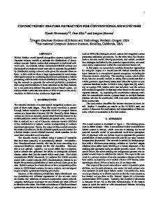
1.4 Our Sonar System In this work, sonar-based modeling aims at the extraction of speci c information from the environment with the objective of reducing the uncertainty associated with odometry errors, and subsequently with navigation. A feature-based model on a sonar array con guration was selected for this task. The idea is to detect a set of common features in the environment, and to use these features as landmarks (or soft beacons), allowing the robot to navigate without loosing its pose, and thus, to keep collecting consistent spatial information for navigation purpose. The generality and applicability of this method depends not only on the accuracy of the sonar model, but also on how frequently, how constant, and how easily detectable the features selected are. In this respect, the environmental features selected are those produced by walls { plane (line), convex edge (edge), concave edge (corner). These environmental features have the characteristics required above, and closed-form solutions exist for properly con gured sonar arrays [20, 15, 11]. Feature detection is based on geometrical relations between two sonars; one of which transmits and receives (T ), and the other only receives the return signal (R). It is assumed that the world geometry is approximately plane-, edge-, or corner-like and that it produces a reproducible pattern of responses on these feature detectors. Figures 1.1, 1.2, and 1.3 depict the geometric analysis involved on the translation from sonar ranging (r1 from the transducer T and r2 from the transducer R) to feature coordinates: edges and corners are recovered as (x,y) (Cartesian coordinate system), and lines are expressed using (r,) (Polar coordinate system). The sonar model procedure, as shown on Figure 1.4, receives as input a reading pair (r1 
r1 ,r2 
r2 ) and outputs, when appropriate, the position evidence (x 

5

Line (r,θ )

sonar cones

T

c (x,y)

a b

R

r 1 = 2c r2 = a + b

Figure 1.1. Line feature model

sonar cones

Edge (x,y)

T c

R

(x,y)

a

r1 = 2 c r2 = a + c

Figure 1.2. Edge feature model

sonar cones

T

Corner (x,y) a c

R

e

(x,y)

b r1 = 2 c r2 = a + b + e

Figure 1.3. Corner feature model

6 TOF sonar data

Measurement space

Feature space

measurement

possible evidence

readings r1

valid pair Measurement filter

r2

r1 r2

+ − + −

line

line model edge model

∆r 1 ∆r 2

edge

corner model

corner

r θ

−+ + −

∆r ∆θ

x y

−+ −+

∆x ∆y

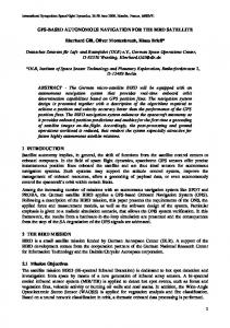
Sonar-based Modeling Procedure: 1. Discard the reading if the re ections (r1 ,r2 ) have no evidence of coming from the same feature; 2. Translate the sonar measurement (r1 ,r2 ) into 3 feature position evidence in feature space, (x,y) for edge and corner features, and (r,) for line feature; 3. Compute the error associated to each feature position evidence by translating the uncertainty from measurement space (
r1 ,
r2 ) to feature space { (
x,
y) and (
r,
).

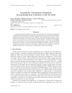
Figure 1.4. Sonar model, from raw sonar data to feature evidence.
x,y 
y) and (r 
r, 
) for the three features. Details about this procedure are presented on Chapter 2 and Appendix A. Several spatial con gurations were considered and are shown on Figure 1.5: (1) a sonar ring with 24 transducers that can execute 3 simultaneous transmissions from equidistant transducers, and all transducers can listen for return signals. (2) a two sonar array with one transducer transmitting and both receiving (Figure 1.5, middle and right frames). The impact of active sonar con guration in feature detection and identi cation tasks are analyzed in Chapter 2.

18 sonar 0

sonar 0

1

1

sonar 0

12

6

24 sonar ring

rotating sonar array (aligned)

active sonar

Figure 1.5. Sonar spatial con gurations.

Chapter 2 Feature Detection and Identification

The goal of extracting features from the environment is to use them as landmarks, or beacons, in navigation tasks. Therefore, features should be selected that are easy to detect and are abundant enough in the environment to permit their utilization as navigational feedback. This work uses lines, corners, and edges extracted from common indoor room features such as vertical planes (walls), corners and convex corners (edges), respectively. These features are not only common in an indoor environment, but they also allow closed-form estimates from time-of- ight (TOF) sonar information. To extract features using sonar, models of the interaction between the ultrasound signal and the environment are required. The physics of these interactions are extremely complex and dependent on the environment, making the derivation of a precise model impossible. The alternative is to create simpler models by relying on some assumptions and introduce restrictions on the applicability of the model. In particular, we assume that the environment is specular to ultrasound. This assumption is imperative to the feature model derivation, and it was shown elsewhere to be not restrictive in practice [13].

2.1 Feature Localization Models All the feature models described here use only range information from a pair of sonars. The range is easily obtained from TOF, since the velocity of sound in air is approximately constant in indoor environments ( 343m=s). One of the sonar pair operates as a transmitter and receiver (T ), returning the range r1 , and the other operates only as a receiver (R), producing r2. The range pair (r1, r2) is then used to compute a position estimate of each possible feature.

2.1.1 Line Feature The line feature hypothesis uses the pair of ranges (r1 , r2 ) and the position and orientation estimate of the transducer T (xT ,yT ,T ) to create a line position estimate (r, ). This transformation is based on two assumptions: the line belongs to a specular surface, thus the angle of incidence is equal to the angle of re ection; and both signals received by the transducers T and R come from the same planar surface.

8 Line (r,θ )

x

θ r

Virtual Image

y T

T’

(x l ,y l )

d

d

R

R’ −α

T

γ

r1 α

r1

R

β

d

r2

Figure 2.1. Line re ection Figure 2.1 depicts the re ections generated by the ultrasonic signal on a planar re ector where T 0 and R0 are virtual images of T and R, respectively. Under these circumstances, (r1 , r2 ) must satisfy the following relations:

q r2 = (r1 ? d sin())2 + (d cos())2 q = r1 2 ? 2r1d sin() + d2 2 + r1 2 ? r 2 2 ! d  = arcsin 2dr1 ! d cos(  ) = arctan r ? d sin() 1

(2.1) (2.2)

where d is the distance between transducers,  is the angle between the line that connects the transducers and the line feature, is the angle between sonar bearings corresponding to r1 and r2 . Given the angle  from Equation 2.1, the position and orientation of the transducer T (xT ,yT ,T ), and the angle ( ) between the transducer T orientation and the normal to the line that connects the transducers, it is possible to compute the line parameters (r, ), referring again to Figure 2.1:

r = xl cos() + yl sin()

(2.3)

 = T + 

(2.4)

9 x

Corner (x c,y c)

Virtual Image

y

R’

T (x c,y c)

d

d

R

T’

T

ξ

γ r2

r1

R

β

d

r1

−α

Figure 2.2. Corner re ection where:

xl = xT + r21 cos(T +  ) yl = yT + r21 sin(T +  )  = +

(2.5) (2.6) (2.7)

2.1.2 Corner Feature The corner feature uses the range pair and the current position and orientation estimate of the transducer T to create the corner position estimate (xc, yc). A corner is composed of two intersecting, orthogonal planar surfaces. It is assumed that all the re ections come from the same corner feature. The re ections of the ultrasonic signal on two planar re ectors forming a right angle corner are shown on Figure 2.2. The relations between sonars ranges are:

q r2 = (r1 ? d sin())2 + (d cos())2 q = r1 2 ? 2r1d sin() + d2 2 + r 1 2 ? r2 2 ! d  = arcsin 2dr1 ! d cos(  ) = ? arctan r ? d sin() 1

(2.8) (2.9)

10 where d is the distance between transducers,  is the angle between the line that connects the transducers and the corner feature, is the angle between sonar bearings corresponding to r1 and r2 , and T 0 and R0 are virtual images of T and R, respectively. As shown, the corner feature ranges share the same relation as the line feature, except by an inverse sign on the angle . The corner parameters are calculated based on the angle  from Equation 2.8, the position and orientation of the transducer T (xT ,yT ,T ), and the angle ( ) between the transducer T orientation and the normal to the line connecting the transducers. Notice that they are identical to the line feature parameters. xc = xT + r21 cos(T +  ) (2.10) yc = yT + r21 sin(T +  ) (2.11)  = + (2.12) Also notice that the orientation of the corner cannot be extracted since r1 and r2 depend only on the corner position (xc, yc) and the transducers' relative position, as shown by the shaded triangle on Figure 2.2.

2.1.3 Edge Feature The edge feature model also uses the pair of sonar ranges and the current position and orientation estimate of the transducer T to create the edge position estimate (xe, ye). The assumptions required for modeling an edge feature are distinct from the previous assumptions. For edge feature modeling, the point of re ection is assumed to be relatively independent of the sonars position, and the edge must be a high curvature convex corner 1. The physical phenomenon that causes the re ections on a sharp edge is modeled as pure diusion, and not specular re ection as on the other features. Figure 2.3 shows typical re ections on a high curvature edge surface, where the following relations are extracted: r r1 r 1 r2 = 2 + ( 2 )2 + d2 ? r1d sin() 2 + r 1 r2 ? r2 2 ! d  = arcsin (2.13) dr1 where d is the distance between transducers,  is the angle between the line that connects the transducers and the edge feature, and T 0 and R0 are virtual images of T and R, respectively. Notice that , the angle between sonar bearings corresponding to r1 and r2, is zero. The following derivation of the edge parameters, similarly to the previous features, uses the angle  from Equation 2.13, the position and orientation of the High curvature in this situation are curvatures with radius the ultrasonic signal transmitted, < 7mm. 1

smaller than the wavelength of

11 x

Edge (x e,y e)

T

y

d (x e,y e)

R

r1 / 2

T

γ

d

α

R

r1 , r2

r2 − r1 / 2 α

Figure 2.3. Edge re ection transducer T (xT ,yT ,T ), and the angle ( ) between the transducer T orientation and the normal to the line that connects the transducers. (2.14) xe = xT + r21 cos(T +  ) ye = yT + r21 sin(T +  ) (2.15)  = + (2.16)

2.1.4 Feature Localization Error To complete the derivation of the feature localization models, it is necessary to estimate the uncertainty associated with each feature parameter; such uncertainty is a function of the uncertainty in the sonar measurements r1 and r2, given by
r1 and
r2 respectively, the non-linear transformations from measurement space to feature space, and the transducers spatial con guration together with beam angles. Two dierent approaches were tested; an analytic approach and a geometric approach. Given the error in sonar measurements, the analytic approach is based on the computation of the maximum possible error generated by the transformations from measurement to feature space. The geometric approach uses the con guration of the transducers, their beam angles, and the uncertainty on their readings to calculate the region in space that might contain the feature correct position. The uncertainty in the feature localization can then be calculated indirectly from the resulting estimate. A brief description of both methods used to estimate the feature localization error follows; a more detailed description can be found in Appendix A. Both approaches are conservative in their error estimate. The analytic method is very conservative since it uses the maximum absolute error of the non-linear feature

12 Feature Error Calculation (Analytic Method): Compute the maximum error of a feature parameter u : u 2 fr; ; xe ; ye ; xc ; yc ;  g by: 1. Calculating the extrema of the feature parameter function fu within the range r1 
r1, and r2 
r2 . 2. Returning the maximum absolute error of the feature parameter (
u), if there was no constraint violation on the measurement range tested; otherwise, ignore this measurement. Feature Error Calculation (Geometric Method): 1. Calculate the region where the sonar re ections could occur, given the sonar measurements range (r1 
r1, r2 
r2 ), the sonar con guration, the beam angles, and the type of feature under analysis. 2. Return the error in the feature localization (
r,
,
xe,
ye,
xc , or
yc) given the above region, if such region exist; otherwise, ignore the measurement.

localization formulas. The geometric method is as accurate as the sonar beam angle selected. The main advantage of the geometric over the analytic approach is the direct association between sensor con guration and precision of the measurement. In principle, this permits the process of computing the feature localization error to be inverted, leading to techniques for selecting the sonar con guration for more precise measurements.

2.2 Extracting Features from Sonar Information As features are extracted from the environment, a ltering process is used to overcome measurement noise. For normally distributed error processes, ltering normally produces better feature hypotheses by fusing measurements over multiple observations [17, 1, 10]. Figure 2.4 depicts the process of extracting feature localization hypotheses from sonar ranging. The ranging information is ltered (Measurement Filter) creating consistent sonar measurement pairs { consistency in this case means that both re ections come from the same feature. Then each pair can be transformed into feature evidence using the feature models. Over time, feature localization evidence from independent observations are fused in a recursive lter. The rst method (method #1 in Figure 2.4) uses Extended Kalman Filters based on the feature models to convert from measurement space to feature-hypotheses automatically. The second method (method #2) initially transforms a measurement into supporting evidence for all three features (line, edge, and corner) using the feature models and then uses Linear Kalman Filters to incorporate the feature evidence into the feature hypothesis

13

Measurement filter valid pair

Measurement space measurement method #1

candidate r2

r1

TOF sonar data readings

r1 − + ∆ r1 r + ∆r 2− 2 method #2

method #1

method #2

line edge corner model model model

Feature space

Fusing Measurement

multiple feature evidence

into Feature Hypothesis Pool

edge corner line r+ − ∆xe xc + − ∆xc −∆r xe + θ+ − ∆ye yc + − ∆yc −∆θ ye + Fusing Evidence into

Feature−hypothesis space multiple feature hypothesis

Feature Hypothesis Pool set of consistent hypothesis

Figure 2.4. Feature localization procedure. pool. The derivation of the extended and Linear Kalman Filters used by the line, edge, and corner features are the subject of Appendix B.

2.2.1 Measurement Space A measurement in this space is composed of two sensor readings (r1 and r2) from the same sonar ring event, where the sonars are in a T=R functional con guration. Moreover, these readings come from re ections on the same feature in the environment. To avoid readings from multiple features, a lter based on a relation derived from the feature models is employed. Equations 2.1, 2.8, and 2.13 express the relation between the sonar re ections (r1 and r2 ), and the distance between the transducers (d) that cannot be violated by any of the features. The formulas below show the constraints imposed on r1 and r2 . 2 2 2 d + r1 ? r2  1 (2.17) 2dr1 2 d + r1r2 ? r2 2  1 (2.18) dr1 These equations evaluate to the same relation since r1 , r2, and d are positive numbers and r1 > d: jr2 ? r1 j  d (2.19) Therefore, all readings that violate this relation are disregarded as measurements, eliminating, to some extent, readings that are not consistent with the feature models.

14 Hypothesis

Evidence

Ph

Pe

Metric = Ph x Pe

Figure 2.5. Feature-hypothesis update metric { one dimensional Gaussians were used here for illustration purposes.

2.2.2 Feature Space and Feature-hypothesis Space In feature space the information is expressed as multiple evidence, composed by line feature evidence (r 
r,  
), edge evidence (xe 
xe , ye 
ye), and corner evidence (xc 
xc, yc 
yc). Multiple hypotheses are generated by transforming each sonar measurement pair (r1 , r2 ) using the respective feature models. Each feature hypothesis represents a feature in the environment, and is obtained by fusing evidence over time and from dierent robot poses. Each hypothesis is interpreted by three Kalman Filters, one for each sonar feature type, creating a feature-hypothesis triple.

2.2.3 Feature-hypothesis Update In the process of updating the feature-hypothesis triple, the fusion process must determine whether a new observation belongs to an existing feature-hypothesis in the pool. The metric used computes the probability that samples drawn from both distributions simultaneously lie in the overlapping volumes, expressing the similarity between the hypothesis and the measurement. This probability is obtained by calculating the product of the overlapping volumes of two 2D-Gaussian distributions (N ((x; y); ((
3x )2; (
3y )2)) for edges and corners, or N ((r; ); ((
3r )2 ; (
3 )2)) for lines) generated by the Kalman Filter estimate and the feature measurement evidence, as shown in Figure 2.5. The metric assumes values between 0 and 1, and is equal to 1 when the distributions are identical, and zero when there is no overlap between them2. A more detailed description on how to select the hypothesis to fuse the new feature evidence follows. Both Gaussian distributions were truncated on the 3 points. And, in the case of one distribution being contained in the other, a factor (thr = 0:3) is added to the metric, biasing the system to avoid the creation of multiple similar hypotheses for the same feature. 2

15 Selecting in which hypothesis to fuse the new observation: 1. Compute the similarity metric for each feature-hypothesis in the pool of hypotheses, and for each feature type; 2. Search for the hypothesis that has the higher metric value; 3. Return the hypothesis' id if its metric value exceeded a threshold (thr = 0:3); otherwise create a new hypothesis.

2.3 Feature Identi cation

The degree of belief in a feature hypothesis is determined by the diagonal terms of the covariance matrix of the corresponding lter (2 < 0:001). When the belief in a feature hypothesis is suciently high, the next step is to identify the feature-type which best accounts for the data. This process is called feature identi cation, and is the last step in feature extraction. The approach used calculates a con dence measurement for each feature in a hypothesis, and selects the feature with a higher relative con dence value. This con dence discrimination measure is calculated as follows: Feature con dence measurement: 1. On the last n measurements (n  20) fused into the hypothesis, use their corresponding sonar con gurations to: (a) Compute which sonar measurements the current lter feature estimate generates; (b) Compare the above measurements with the original measurements fused, by using the same metric used to select in which hypothesis to fuse a new evidence; 2. Compute each feature con dence by taking the average of all the metric values over the n measurements; 3. Select the feature with the best con dence value, higher (0.2) than the second best on this hypothesis.

The success of this approach depends on the quality of the information fused. The feature identi cation process is computational expensive; it requires information from multiple sonar con gurations and sometimes even dierent robot poses to correctly distinguish the three possible features. Therefore, any passive sensing procedure is in principle inappropriate for this task and the acquisition of information should be active based on previous knowledge of how and where the relevant information can be acquired. This knowledge can be obtained in part by analyzing the task requirements and can be augmented by reasoning on the basis of past experiences.

Chapter 3 Experiments

3.1 Experiments in Feature Localization and Identi cation All the experiments reported here were obtained using a 2D simulator of sonar re ections on a specular environment composed of lines, edges, and corners features. The simulator uses the feature models, a simple model of the ultrasonic sensor that considers range and beam angle, and a Gaussian noise process to corrupt the sonar returns (Appendix C). This simulator was developed for testing the feature localization approaches based on linear and Extended Kalman Filters and also to characterize the importance of sonar con guration in feature extraction. The experiments are divided in three parts. The rst part presents results of feature extraction at dierent locations of the same environment using the Extended Kalman Filter and the Linear Kalman Filter approach, followed by a comparison of both methods. The second experiment explores the detection of features by fusing information from multiple robot poses and possible active sensing strategies. And the last experiment addresses the impact of sonar con guration on feature extraction. All the experiments were done using the analytical method in the feature error calculation.

3.2 Part 1: Experiments on Feature Extraction and Filtering Approaches In this experimental part, we selected 3 robot poses in the same environment, composed of 12 features (lines, corners, and an edge), approximately 6 by 3 m. All simulator snapshots were taken after 3 full scans ( 300 rings { 4 rings every 15 degrees, interleaving TR and RT con gurations) of a rotating 2-sonar array. In the gures, the robot is represented by the \T" shaped bar, and the sonars, localized in the ends of the bar (d = 0:6m), are aligned in the direction of the robot. The absolute localization error of the features identi ed at the end of each full scan is reported on the corresponding tables (a dash on the table represents a feature not identi ed at that moment). No feature was misclassi ed on the following examples.

3.2.1 Extended Kalman Filter Approach An Extended Kalman Filter (EKF) is employed when the system cannot be adequately described by a linear model. In our case we used a rst-order EKF to directly estimate the position of a 2D feature (line, edge, or corner) in a static

17

Figure 3.1. Simulator snapshots of a rotating 2-sonar array using the EKF method. environment, using the discrete-time measurements obtained from the two sonar sensors (r1 , r2 ), as described in Chapter 2 and Appendix B. Figure 3.1 presents snapshots from 3 robot poses after 3 full scans as previously described. The left column presents all the hypothesis gathered during the scans and the right column shows the features identi ed. As shown, the system was able to classify correctly several nearby features (< 2 m from the robot). The absolute localization error of the features extracted on each sonar scan is reported on Table 3.1, where the localization error is on average one order of magnitude better than the uncertainty of the raw data (1% of the readings). These tables directly correspond to the previous snapshots.

18 Scan # 1 2 Total # of features identi ed 3 3 Total # of hypothesis created 9 9 Right-lower x < 0.001 0.001 Absolute edge y 0.006 0.004 feature Bottom r 0.036 0.002 error wall  0.011 < 0.001 r; x; y in m Top r 0.008 0.010  in rad wall  0.003 0.003 Scan # Total # of features identi ed Total # of hypothesis created Bottom r Absolute wall  feature Left-side r error wall  r; x; y in m Top r  in rad wall  Scan # Total # of features identi ed Total # of hypothesis created Right-side r Absolute wall  feature Bottom r error wall  r; x; y in m Top r  in rad wall 

1 3 8 0.013 0.007 0.003 0.002 0.004 0.002 1 3 10 0.006 0.005 0.013 0.003 0.005 0.001

2 3 8 0.008 0.003 0.004 0.003 0.003 0.002

3 3 9 0.002 0.004 0.011 0.004 0.010 0.004

4 3 9 0.003 0.008 0.002 0.001 0.007 0.003

3 4 3 3 9 9 0.008 0.002 0.003 0.001 0.001 0.007 0.002 0.006 0.003 < 0.001 0.002 < 0.001

2 3 4 3 3 3 10 10 10 0.005 < 0.001 < 0.001 0.004 < 0.001 0.002 0.027 0.033 0.032 0.006 0.008 0.008 0.009 0.006 0.009 0.002 0.001 0.002

Table 3.1. Feature extraction results from 2-sonar array using the EKF method.

3.2.2 Linear Kalman Filter Approach In this section, we present the same case examples as before, but with the Linear Kalman Filter (KF) approach. As described in Chapter 2 and Appendix B, a Linear Kalman Filter was employed after computing the feature position and error associated with each pair of measurements (r1, r2 ), simplifying the data fusion by executing directly in feature space (linear data fusion). Figure 3.2 presents snapshots from the same 3 robot poses as before. The left column presents all the hypothesis gathered during the scans and the right column shows the features identi ed. Again, the system was able to classify correctly almost all nearby features (< 2 m from the robot). Table 3.2 reports the absolute localization error of the features extracted on each sonar scan, and the localization error is on average in the order of millimeters.

19

Figure 3.2. Simulator snapshots of a rotating 2-sonar array using the KF approach.

3.2.3 Comparison Between Filtering Approaches Both ltering methods, the EKF and the KF, demonstrated to be eective in localizing the features given the sonar readings. They were equally able to localize line, edge, and corner features with an average absolute error in the order of millimeters. The only discrepancy was in the number of features identi ed, and in the number of evidence required by the ltering process before an identi cation; more features where identi ed using the KF approach, however, the EKF approach was in some cases faster identifying the features. The EKF method was better identifying line and edge features, but it identi ed less features by failing to identify the corner features. This happened because the variance of the corner feature was higher than the threshold used in identi cation

20 Scan # Total # of features identi ed Total # of hypothesis created Right-lower x edge y Absolute Right-lower x feature corner y error Bottom r r; x; y in m wall   in rad Top r wall 

1 0 9 { { { { { { { {

2 2 10 0.002 0.006 0.010 0.019 { { { {

3 4 10 0.002 0.006 0.008 0.017 0.004 0.002 0.023 0.007

4 4 10 0.003 0.010 0.017 0.027 0.021 0.006 0.013 0.004

Scan # Total # of features identi ed Total # of hypothesis created Left-side r wall  Top r Absolute wall  feature Bottom r error wall  r; x; y in m Left-upper x  in rad corner y  in rad Left-lower x corner y

1 2 8 0.001 0.006 0.001 0.001 { { { { { {

2 3 4 4 5 5 8 9 9 0.002 0.002 0.007 0.001 < 0.001 0.010 0.005 0.001 0.002 0.002 < 0.001 < 0.001 0.014 0.011 0.011 0.006 0.004 0.005 0.001 0.002 < 0.001 0.005 0.004 0.006 { 0.006 0.004 { 0.017 0.008

Scan # Total # of features identi ed Total # of hypothesis created Right-side r Absolute wall  feature Right-upper x error corner y r; x; y in m Top r  in rad wall 

1 1 10 0.013 0.011 { { { {

2 3 4 2 3 3 10 11 10 0.010 0.003 0.011 0.009 0.001 0.008 0.001 0.001 0.003 0.006 0.005 0.005 { 0.004 0.003 { < 0.001 < 0.001

Table 3.2. Feature extraction results from 2-sonar array using the KF approach. (2 < 0:001). And, since the data fused were similar in both approaches, the higher variance may be explained by the rst-order EKF been unable to cope with the nonlinearities of the system. Therefore, the implementation of a second-order EKF may be necessary for the identi cation of corner features. The main advantage of using an extended Kalman Filter is to have a direct implementation, where the transformation from measurement space to feature space is automatically done by the lter (direct approach). However, the lter derivation is usually dicult, especially when a high-order lter is necessary, and in several cases it is preferable to separate the space transformation from the ltering process (indirect approach). After testing both methods, we conclude that, in our application, the direct approach was easier to implement than the indirect approach; however the

21 analyze of the feature error associated with each measurement pair and sensors' con guration gave us new insights on possible active sensing strategies to maximize the information extracted from the measurements.

3.3 Part 2: Feature Extraction over Multiple Poses

Figure 3.3. Simulator snapshots of a rotating 2-sonar array over multiple poses, using the KF approach. The objective of this experiment was to show how an active sensing strategy could improve and accelerate the feature extraction process. The experiment is

22 divided in 3 parts, corresponding to the line, edge, and corner feature extraction procedures. The data were collected over 5 aligned, equally spaced robot poses, and the sensors' orientation was kept constant during the experiment. Figure 3.3 presents 3 simulator snapshots of each experimental part at the extrema and middle robot poses. The rightmost snapshots corresponds to the rst sonar ring, the middle snapshots to third ring event, and the leftmost to the fth one. In this experiment, the line feature was identi ed after 3 sonar rings (or evidence fused) with absolute feature error in the order of millimeters (
r = 0:003,
 = 0:002). Notice that this feature was not identi ed in the previous experiments from a single robot pose (see Figure 3.2 and Table 3.2, rst experiment). Similarly, the edge feature was identi ed after 4 evidence being fused with absolute feature error of (
x < 0:001,
y = 0:001); and, as before, the system was unable to identify this feature from a single pose (see Figure 3.2 and Table 3.2, last experiment). The corner feature required 6 evidence, contrasting with 17 evidence needed from a xed, near ideal robot pose, with absolute feature error of (
x = 0:001,
y = 0:003).

3.4 Part 3: Comparison Between Sonar Array Con gurations

Figure 3.4. Simulator snapshots of a rotating 2-sonar array ( rst three snapshots) and a 24 sonar ring (last snapshot). Following the experimental procedure of the rst experiment (Section 3.2), Figure 3.4 compares the performance of a rotating 2-sonar array and a 24 sonar ring.

23 The rst snapshot shows all the features localized, and the second (left on the gure) presents the features identi ed (all 5 correctly identi ed). In the bottom row, the left snapshot presents the raw data used on the previous examples (dots). The last snapshot (right on the picture) presents all the hypotheses created by a ring after the same amount of rings, but, in this case, no feature was identi ed. Both sonar con gurations have advantages and drawbacks. As demonstrated, the 2-sonar array not only detected more features than the ring, but also correctly identi ed all the nearby features. On the other hand, the ring was able to localize 4 out of 5 features faster than the 2-sonar array, and it is an eective con guration for obstacle avoidance. In a navigation task a synergetic relation can be created where a sonar ring can contribute by directing a rotating sonar array to places with high probability of nding a landmark, navigating reliably and avoiding obstacles.

Chapter 4 Conclusions and Future Work

This technical report presented a procedure based on multiple hypothesis testing for localizing and identifying indoor features using sonar data, demonstrating that accurate feature information can be acquired with the use of an adequate sonar model and con guration. The results presented shows a direct association between sensor con guration and localization precision, suggesting the possibility of creating sonar controllers capable of extracting better information by actively exploiting sensor con guration.

4.1 Active Sonar System

An active sonar sensor is being developed to further validate the results presented in here. Figure 4.1 shows our mobile robot and Figure 4.2 shows the functional diagram of the two-sonar array (left), where both transducers are mounted on an axis that can pan and tilt, and each transducer has an extra pan degree of freedom. The pan and tilt of the axis aords the localization of features at any direction, and at any height respectively. In addition, the extra verge degree of freedom (DOF) on each transducer allows the system to adjust the sonar con guration to feature distance and feature type, thereby producing better quality measurements. In the right side of Figure 4.2, a TRC stereo head system that will serve as testbed for the 2-sonar active array system is presented. More details about our mobile robot (Isaac) and the active sonar system can be found in Appendix D.

Figure 4.1. Mobile robot and proposed active sonar.

25

sonar 0

1

Figure 4.2. Active sonar system This work supports robot navigation, by allowing the identi cation of landmarks even in presence of measurement noise. By detecting common features in indoor environments and using these features as landmarks, a robot can navigate reliably, recovering its pose when necessary.

Appendix A Feature Error Calculation

A.1 Analytic Method The analytic approach is based on the computation of the maximum error on feature space, given the measurement pair (r1; r2), their correspondent error (
r1 ;
r2), and the non-linear transformations from measurement to feature space. The algorithm below summarizes the procedure used to transform errors in measurement space to feature space. Feature Error Calculation (Analytic Method): Compute the maximum error of a feature parameter u : u 2 fr; ; xe ; ye ; xc ; yc ;  g by: 1. Calculating the extrema (er1 i ; er2 i ) : i 2 E , where E is the set of all possible maxima and minima of the feature parameter function fu within the range r1 
r1 , and r2 
r2 . 2. Returning the maximum absolute error of the feature parameter (
u), if there was no constraint violation on the measurement range tested; otherwise, ignore this measurement.
u = max jfu(r1; r2 ) ? fu(er1 i ; er2 i)j i2E

The non-linear transformations from measurement space to each feature (previously described in Chapter 2), their partial derivatives with respect to the measurement, and the tests used to identify violation of constraints on the range of possible measurements (u 
u) are presented in the following sections. Notice that r1 and r2 represent variables now and not a measurement. Mathematical software packages were employed on the calculation of the extrema. Mathematica1 was the software package used, except for the extrema calculation relative to the line feature ( @r@r1 = 0) that was solved using Maple2, because Mathematica was unable to solve it. The solutions obtained present zeros that are not zeros of the initial function; the extra roots are introduced by the presence of square roots in the derivatives. Therefore, an online check of the solutions to determine the true extrema of the 1

c Wolfram Research, Inc. Mathematica 2:2 -

2

c Waterloo Maple, Inc. Maple V release 2 -

27 initial function is necessary. Moreover, there are physical factors that restrict the extrema, such as r1 and r2 being positive measurements limited by the sonar range, d being limited by the diameter of the mobile robot, the origin frame being conveniently selected to reside out of the robots space, and  being limited to the transmitter cone angle.

A.1.1 Edge Feature  The feature parameter functions are:

2 + r1 r2 ? r2 2 ! d  = arcsin + ; dr1 xe = xT + r21 cos(T +  ) ; ye = yT + r21 sin(T +  )

(A.1) (A.2)

where (xT ,yT ,T ) are the position and orientation of the transducer T , is the angle between the transducer T orientation and the normal to the line that connects the transducers, and d is the distance between transducers.  The corresponding partial derivatives are: 2 2 @ = @ = r r1 ? 2 r2 r?d +2 r2 ; @r1 d r 2 1 ? (d +r1 r2?r22 )2 @r2 d r 1 ? (d2 +r1 r2 ?r22 )2 ; 1 1 d2 r1 2 d2 r1 2

1 0 B (d2 ?r22 )(r d2 +r1 r2 ?r2 2 ) cos(T + ) ? r2 sin(d r1T + ) CCA r1 B @ 2 (d2 +r r ?r 2 )

1 2 2 d2 r1 3 1? d2 r1 2 @xe = + @r1 2 r 2 1 ? (d2 +rd12rr21?2 r2 2) cos(T + ) ; 2 1 0 B (r1 ?2 r2 ) (dr2 +r1 r2?r2 2) cos(T + ) (r1 ?2 r2 ) sin(T + ) CC r1 B A @? 2 2 (d2 +r1 r2?r2 2)2 ? d r1 1? d2 r1 2 d r1 @xe = ; @r2 2 1 0 B (d2 ?r22 )(rd2+r1 r2?r22 ) sin(T + ) r2 cos(T + ) CC r1 B @ 2 3 (d2 +r1 r2+r22 )2 ? d r1 A 1? d2 r1 2 d r1 @ye = + @r1 2 r 2 1 ? (d2 +rd12rr21?2 r2 2) sin(T + ) ; 2

@ye = @r2

1 0 B (r1 ?2 r2 ) (r d2 +r1 r2 ?r2 2 ) sin(T + ) T + ) C CA + (r1?2 r2)d cos( r1 B ? @ r1 2 d2 r1 2

28

1? (d2 +rd12rr21?2r2 2 )

2

 Extrema calculation:

The extrema of a bounded 2D function could be on the boundaries or on the interior. On the boundaries, the extrema could be at the four corners, or at the edges of the region de ned by (r1 
r1 and r2 
r2 ). All the possible extrema points within the measurement range are used to compute the maximum absolute error of the feature parameter.

{ Finding extrema on the borders:  Solving @r@1 = 0 The function  is strictly monotonic with respect to r1 .

 Solving for @r@2 = 0 e  Solving @x @r1 = 0

r2 = r21

q

2 d2 r22 (?d2 + 2 r22 ? d2 cos(2 (T + ))) sin(T + )2 r1 = r2  d2 ? 2 r22 + d2 cos(2 (T + )) e  Solving @x @r2 = 0

r2 = r21 ; r q r1  4 d2 + r1 2  4 d2 r12 sin(T + )2 r2 = 2

 Solving @y@r1e = 0 r1 = r2 

q

2 d2 r2 2 (?d2 + 2 r22 + d2 cos(2 (T + ))) cos(T + )2 d2 ? 2 r22 ? d2 cos(2 (T + ))

 Solving @y@r2e = 0

r2 = r21 ; r q r1  4 d2 + r12  4 d2 r12 cos(T + )2 r2 = 2

29

{ Find interior extrema:  Solving @r@1 = 0 and @r@2 = 0; @xe e  Solving @x @r1 = 0 and @r2 = 0;  Solving @y@r1e = 0 and @y@r2e = 0.

The functions  , xe, and ye are strictly monotonic with respect to r1 and r2, thus presenting no solution.

 Measurements' constraints:

Derived from the previous equations, the constraints imposed are:

d; r1 6= 0 ;

jr2 ? r1 j < d ; r2 > d

A.1.2 Corner Feature  The feature parameter functions are:

2 + r 2 ? r2 2 ! d 1  = arcsin + 2dr1

(A.3)

The other parameters functions xc and yc are the same as in the case of an edge feature (Equations A.1 and A.2).  The corresponding partial derivatives are: @ = ? r r2 @ = ?dr2 + r12 + r22 ; ; 2 @r1 2 d r 2 1 ? (d2 +r12 ?r22 ) @r2 ( d2 +r1 2 ?r2 2 )2 d r1 1 ? 4 d2 r12 1 4 d2 r1 2

1 0 B (d4 ?r14 ?2rd2 r22 +r24) cos(T + ) sin(T + ) CC ? d A r1 B @ 2 4 d2 r1 3 1? (d2 +4rd122r?1r22 2 )

@xc = @r1 r

@xc = @r2 @yc = @r1

2 2 2 2 2 1 ? (d +4rd12 r?1r22 ) cos(T + ) ; 2 1 0 C B 2 2 2 r B r2 (d +rr1 ?r2 ) cos(T + ) + r2 sin(T + ) C 1

@

2 d2 r1 2 1? (d2 +4rd122r?1r22 2 )

2

d r1

+

A

; 2 0 1 B (d4 ?r14 ?2rd2 r22 +r24) sin(T + ) cos(T + ) CC + d A r1 B @ 2 4 d2 r1 3 1? (d2 +4rd122r?1r22 2 )

2

+

30

r

2

1 ? (d2 +4rd122r?1r222 ) sin(T + ) ; 2 1 0 C B 2 2 2 r B r2 (d +rr1 ?r2 ) sin(T + ) ? r2 cos(T + ) C 1

@

2 d2 r1 2 1? (d2 +4rd122r?1r22 2 )

2

d r1

A

@yc = @r2 2  Extrema calculation: { Finding extrema on the borders:  Solving @r@1 = 0 q r1 =  d2 ? r2 2  Solving for @r@2 = 0 r2 = 0 @xc  Solving @r1 = 0 r q r1 =  d2 + r2 2  2 d2 r2 2 sin(T + )2 c  Solving @x @r2 = 0 r2 = 0 r ; q r2 =  d2 + r12  2 d2 r12 sin(T + )2  Solving @r@y1c = 0 r q r1 =  d2 + r2 2  2 d2 r2 2 cos(T + )2  Solving @r@y2c = 0 r2 = 0 r ; q r2 =  d2 + r1 2  2 d2 r1 2 cos(T + )2 { Find interior extrema:  Solving @r@1 = 0 and @r@2 = 0; @xc c  Solving @x @r1 = 0 and @r2 = 0;  Solving @r@y1c = 0 and @r@y2c = 0. The functions  , xc, and yc are strictly monotonic with respect to r1 and r2, thus presenting no solution.  Measurements' constraints: Derived from the previous equations, the constraints imposed are: d; r1 6= 0 ;

jr2 ? r1 j < d

31

A.1.3 Line Feature  The feature parameter functions are:  = T +  ; r = xl cos() + yl sin() The parameters functions xl , yl , and  are the same as in the case of a corner feature (Equations A.1, A.2, and A.3).  The corresponding partial derivatives are: The partial derivatives of xl , yl , and  are similar to the ones presented on the corner feature (Section A.1.2), and the partial derivatives of  are also similar to the ones for  , because the  and  functions only dier by a constant T .

! @r = 1 + d2 ? r1 2 ? r22 (x sin( + ) ? y cos( + )) + T T T T @r1 2 2 d r1 2 (d2 ? r12 ? r2 2) (d2 + r12 ? rr22) (xT cos(T + ) + yT sin(T + )) ; 2 4 d2 r13 1 ? (d2 +4rd122r?1r222 ) @r = r2 (d2 + r12 ? r2 2) (xTrcos(T + ) + yT sin(T + )) + 2 @r2 2 d2 r12 1 ? (d2 +4rd122r?1r222 ) r2 (xT sin(T + ) ? yT cos(T + )) d r1

 Extrema calculation: { Finding extrema on the borders:  Solving @r@r1 = 0:

In this case, it is equivalent to solve the polynomial:

a1 r18 + a2 r1 6 + a3 r14 + a4 r12 + a5 = 0 ; where the coecients are: a1 = ?2 d (xT sin(T + ) ? yT cos(T + )) +d2 + xT 2 + yT 2 ; a2 = ?4 d2 x2T sin(T + )2 + yT2 cos(T + )2 +   8 d2 xT yT sin(T + ) cos(T + ) ? 2 d2 d2 + r22 +   2 d 3 d2 + r22 (xT sin(T + ) ? yT cos(T + )) ;     a3 = 2 d2 ? r22 4 d2 x2T sin(T + )2 + yT2 cos(T + )2 ?  2 2  2 2 d2 ! 2 8 d xT yT sin(T + ) cos(T + ) ? d ? r2 xT + yT ? 2 ?







32

d 3 d2 + r22 (xT sin(T + ) ? yT cos(T + )) ;    a4 = (d ? r2)2 (d + r2 )2 ?4 d2 x2T sin(T + )2 + yT2 cos(T + )2 + 8 d2xT yT sin( T + ) cos(T + ) +   2 d d2 ? r22 (xT sin(T + ) ? yT cos(T + )) ;   a5 = (d ? r2)4 (d + r2 )4 x2T + yT2

The solution is:

 p  r1 =  ?9 a2 p6 aux1 p4 aux2 + aux23=4 3  27 a22 p3 aux1paux2 ? p p p 72 a3 a1 3 auxp1 aux2 ? aux2 542=3aux 1 2=3 a1 + p p p 18 aux2 a1p3 54 a2 a4 ? 72p aux2 a1 2 3 54 a5 ? p p 6 aux2 a1 3 54 a3 2 + 324 3 aux1 a2 a1 a3 ? 1=2 p 1=2 pp pp 6 = 648 3 aux1 a1 2a4  81 3 aux1 a2 3  p p  6 a1 aux1 1=12 8 aux2 ; where the auxiliary variables are:

aux1 = ?p 9 a3a2 a4 ? 72 a5 a3 a1 + 27 a42 a1 + 27 a5 a2 2 + 2 a33 + 3 3 27 a44 a1 2 + 6 a22 a42 a5 a1 + 192 a2 a4 a5 2a1 2+ 80 a2 a4 a5 a1 a3 2 ? 18 a3 a2 a4 3a1 ? 18 a3 a23 a4 a5 ? 144 a5 a3 a12 a42 ? 144 a52 a3 a1 a2 2 + 4 a23 a43 ? 256 a53 a13 + 27 a52 a24 ? a2 2a4 2 a32 + 128 a52 a12 a32 ? 16 a5 a1 a3 4 + 1=2 4 a42 a1 a3 3 + 4 a5 a22 a3 3 ; p p aux2 = 27 a22p3 aux1 ? 72 a3 a1 3paux1 + 2 542=3paux12=3 a1 ? 36 a1 3 54a2 a4 + 144 a12 3 54a5 + 12 a1 3 54a3 2

 Solving for @r@r2 = 0 r2 = 0  ;      r2 =  d2 + r1 2 xT 2 + yT 2  2 d2 r1 2 xT 2 + yT 2

1=2 1=2 q 2 2  2 = xT + y T (xT sin(T + ) ? yT cos(T + ))

{ Find interior extrema:  Solving @r@1 = 0 and @r@2 = 0;  Solving @r@x1l = 0 and @r@x2l = 0;  Solving @r@y1l = 0 and @r@y2l = 0;  Solving @r@1 = 0 and @r@2 = 0;

33 r1

Measurement Space

2 ∆ r2 2 ∆ r1

r1

d

d

r2

contraint

r2

| r2 − r1 | < d

Figure A.1. Constraint on the Sonar Measurements

 Solving @r@r1 = 0 and @r@r2 = 0. The functions  , xl , yl , and  are strictly monotonic with respect to r1 and r2 . The function r is also strictly monotonic with respect to r1 and r2 , as determined by a geometrical analysis presented on Section A.2.3. { Measurements' constraints: Derived from the previous equations, the constraints imposed are:

xT ; yT 6= 0 ;

d; r1 6= 0 ;

jr2 ? r1j < d

A.1.4 Characteristics of the Analytic Approach The three main characteristics of this method are: its simplicity (the extrema for the error functions have closed-form solutions); the use of the maximum absolute error, making it a conservative method; and the ease of detecting measurements that violate model constraints. To illustrate the last characteristic, Figure A.1 depicts the limitation imposed by the constraint jr2 ? r1j < d. As shown, the distance between transducers (d) and the error in the measurements (
r1;
r2 ) are related limiting factors. The larger the distance between transducers, the more variance in the measurements can be supported, thus, causing measurements from more distant features not to be discarded.

34

A.2 Geometric Method This method computes the feature space error by means of geometric analysis. It uses the con guration of the transducers, their beam angles, the sonar readings, the uncertainty on the sonar readings, and the model of the feature under analysis (line, edge, or corner) to estimate the region in space that might contain the feature correct position. The uncertainty in the feature localization can then be calculated indirectly from the resulting estimation. The algorithm below summarizes the procedure used to transform errors in measurement space to feature space. Feature Error Calculation (Geometric Method): Compute the maximum error of a feature parameter u : u 2 fr; ; xe ; ye ; xc ; ycg by: 1. Calculating the region where the sonar re ections could occur, using the sonar measurements range (r1 
r1 , r2 
r2 ), the transducers con guration, their beam angles, and the type of feature under analysis. 2. Returning the maximum absolute error in the feature parameter (
u) given the above region, if such region exist; otherwise, ignore this measurement.

The region where the sonar re ection could occur, given a measurement pair (r1 
r1; r2 
r2), changes depending on the type of feature under analysis. The geometrical analysis used on the calculation of this region is described on the following sections.

A.2.1 Edge Feature

In the case of an edge feature, as shown in Figure A.2, both r1 and r2 re ections occur exactly on the edge. In this situation, the error region is limited by the intersection of the transmitter cone with the receiver cone, and by the error region imposed by the measurements (r1 ; r2). Considering the measurement r1, the error region is delimited by two circular arcs generated by x2 + y2 = r2 ; r = 21 (r1 
r1) : In the case of the measurement r2 , the error region is bounded by two elliptical arcs given by: x2 + y2 = 1 ; a = 1 (r 
r ) ; b = 1 q(r 
r )2 ? d2 ; 2 2 a b 2 2 2 2 where d is the distance between transducers. The error in feature space (
xe ;
ye) is obtained by computing the maximum absolute error in x and y directions, respectively. For an edge feature, the possible extrema are on the intersection between circles, ellipses, and sonar cone boundaries, or on the external circle or ellipse, as shown on the left diagram of Figure A.2.

35 x ∆r 1 y

sonar cone boundaries

Edge (x e ,y e) T

circles

R

∆ ye

elipses

measurement

∆ xe

Figure A.2. Edge error x Corner (x c ,y c )

reflection boundary

∆r 1

y T

R

circles ∆ yc measurement sonar cone boundary ∆ xc

Figure A.3. Corner error

A.2.2 Corner Feature As shown in Figure A.3, only the r1 re ection occurs on the corner. Therefore, the x and y position of the corner is contained in the transmitter cone, on the region limited by the uncertainty in the measurement r1 (
r1). Moreover, because the corner feature is a right-angle corner, the r2 re ection has parallel segments, and the above region can be further limited by the receiver's cone boundaries. Similarly to the edge feature, the corner error (
xc;
yc) is the maximum absolute error in the x and y directions, respectively. In this case, the possible extrema are on the intersection between the circles, the transmitter boundaries, and the re ection boundary, or on the external circle, as depicted on Figure A.3.

36 line 1

Line (r , θ)

r’

x

line 1’

∆ r = max (r ’’ − r , r − r ’ )

r line 2

measurement

r ’’

y

line 1

T

∆θ line 2

R

receiver limits transmitter limits line 2’

Figure A.4. Line error

A.2.3 Line Feature On the line feature, the r1 re ection occurs on the transmitter cone and the r2 re ection occurs on the intersection of the transmitter and receiver cones. Both re ections are limited by the error region imposed by the measurements (r1 ; r2), as described before is Section A.2.1. The error region is delimited by the transmitter and receiver limit lines, as presented in Figure A.4, corresponding to possible r1 and r2 re ections, respectively. As before, the line error (
r;
) is calculated based on the maximum absolute error in r and , respectively. Given that a possible line has to be tangent to the circles produced by the r1 re ection, and also tangent to the ellipses produced by the r2 re ection, both errors (
r;
) can be obtained from the limit lines, as demonstrated by the diagram on the left of Figure A.4 where the possible extreme lines are line 1, line 2, line 10, and line 20. Notice that depending on the position of the referential, a combination of lines dierent than the pair (line 1; line 2) will generate the maximum
r, but limit lines have always r1 or r2 at an extreme value.

A.2.4 Error Minimization In measurement space, the error associated with the measurements r1 and r2 is directly proportional to the measurements' value,
r1 = pr1 ;


r2 = pr2 ;

p  0:01

Therefore, to obtain a more precise measurement, the sensors should be closer to the object being measured. As shown in the previous sections, in feature space, not only the sensor distance to a feature but also the con guration of the sensors, and the feature type

37 play an important role on feature error minimization and on feature characterization. Some techniques used in radar systems that exploits the con guration of the antennas to improve measurement quality can also be applied here to the sonar system. In the case of an edge or line feature, a more precise measurement is obtained when the overlap between the receiver and transmitter cones is minimized by rotating the transducers, or by increasing their distance (d). This is also true for the corner feature case, except that the receiver and transmitter cones do not necessarily need to overlap, because the error region is produced by the re ection boundary, and not by the receiver cone boundary. All these facts can be used on the design of active sonar sensor controllers.

A.3 Comparison Both approaches are conservative in their error estimate, since they use the maximum absolute error. The analytic method uses the maximum absolute error derived from the extrema values of the non-linear feature localization formulas, and its application is limited to the constraints imposed to the measurements. The geometric method, in the other hand, uses the sonar con guration and the sonar beam angle estimate to calculate the maximum absolute error, thus being as conservative and accurate as the sonar beam angle selected. The main advantage of the geometric over the analytic approach is the direct association between sensor con guration and precision of the measurement, allowing for the possibility of inverting the problem and selecting the sonar con guration to obtain a more precise measurement.

Appendix B State Estimation - Kalman Filter

A Kalman lter is de ned by Maybeck in [17] as an optimal recursive data processing algorithm. It produces an optimal estimate of the state variables of the system by recursively combining all available measurement data. Its applicability is constrained to situations where the dynamics of the system and measurement devices, together with the statistical description of the noises and uncertainties associated with them, and the initial state of the system are known. The Kalman lter's main importance as a data processing algorithm relies on its optimality and recursive characteristic. A Kalman lter is optimal not only because it uses all the information available, even the least precise measurements, but because it produces the unique best estimate of the state variables when the system dynamics can be described by a linear model, and the system and measurement noises are white and Gaussian. The recursive characteristic of the lter has practical importance, because it does not require all previous data to be saved and reprocessed at each new measurement. In practice, the Kalman lter can be used even when some of the constraints presented above are violated. Extra ltering can be used to change a system with time or frequency correlated noise into a linear system with white noise. Gaussian noise is a physically plausible and practical assumption. And, in case of lack of statistical information about the noise process, there is no better option than to assume Gaussian noise [17]. The Kalman lter can be also compensated to overcome inadequacies on the system and measurement devices models, and extended to address systems that are better described by nonlinear models [18, 1]. The nomenclature used in this paper to describe both the Kalman lter (linear system) and the Extended Kalman lter (nonlinear system) follows the one used by Bar-Shalom in [1]. Figure B.1 presents the nomenclature used on a Kalman lter state estimation cycle, where the system, the control, and the discrete-time Kalman lter estimation algorithm (shaded area) are depicted. For a formal mathematical description of Kalman lters see [17, 1, 10, 18], and, in special, as an introductory reading refer to Maybeck [17]. In this paper, the Kalman lter was used to estimate the position of a 2D feature (line, edge, or corner) in a static environment, using the discrete-time measurements obtained from two sonar sensors, directly (nonlinear case), or indirectly (linear case), as described in Chapter 2. In the following lter implementations, the system has no dynamics and no controller, because the features are static and their positions are computed in global coordinates, reducing the Kalman lter algorithm to a recursive form of a least-square estimator [1].

39

At time t k

System

At time t k+1

State

State

Measurement

χ (k)

χ(k+1)

ζ (k+1)

Control

Controller

u(k)

Estimation Algorithm

State’s Estimation

State estimate

State prediction

χ^ (k|k)

χ^ (k+1|k)

State Covariance Computation

State error covariance P(k|k)

State prediction covariance P(k+1|k)

Measurement prediction ζ^ (k+1|k)

Innovation covariance S(k+1)

Updated state estimate χ^ (k+1|k+1)

Innovation ν (k+1)

Filter gain W(k+1)

Updated state covariance P(k+1|k+1)

Figure B.1. Kalman lter - state estimation cycle

B.1 Extended Kalman Filter

The Extended Kalman lter (EKF) is used when the system cannot be adequately described by a linear model. The idea behind the method is to better follow the system's reference state trajectory, allowing for the use of linear perturbation techniques; therefore, the EKF linearizes about each new state estimate to produce a new and better state trajectory for the estimation process [18, 1]. The following are the general equations of the rst-order Extended Kalman lter algorithm, and the simpli ed EKF version implemented:  System: (k + 1) = f [k; (k)] + g[k; u(k)] + v(k) Taking into account that the process under study is static ( f [
] = (k) ), does not have a controller ( g[
] ), and consequently does not present process noise ( v(k) ), the equation above becomes: (k + 1) = (k)

 Measurement:

 (k + 1) = h[k + 1; (k + 1)] + w(k + 1)

The nonlinear function h transforms state space variables of a feature (line, edge, or corner) to measurement space variables (sonar readings, (r1, r2)). The measurement noise w represents an additive, zero-mean, and white noise.

40

 State estimation and covariance computation: { State prediction:  ^(k + 1jk) = f [k; ^(kjk)] + g[k; u(k)] Similarly to the system's state equation above, ( f [
] = ^(kjk) ), and ( g[
] = 0 ), resulting in:  ^(k + 1jk) = ^(kjk) { State prediction covariance: h i P(k +1jk) = f(k) P(kjk) fT (k)+Q(k) ; f(k) =4 rf T (k; ) T=^(kjk) where f(k) is the Jacobian of the vector f , and Q(k) is the system noise covariance matrix. As before, this equation can be simpli ed to: P(k + 1jk) = P(kjk)

{ Measurement prediction: ^(k + 1jk) = h[k + 1;  ^(k + 1jk)] { Innovation:

 (k + 1) =  (k + 1) ? ^(k + 1jk)

{ Innovation covariance: S(k + 1) = h(k + 1) P(k + 1jk) hT(k + 1) + R(k + 1) ; h

i

h(k + 1) = rhT (k + 1; ) T=^(k+1jk) where h(k+1) is the Jacobian of the vector h, and R(k) is the covariance

matrix of the noise associated with the measurements. { Filter gain: W(k + 1) = P(k + 1jk) hT(k + 1) S?1(k + 1)

{ Updated state estimate:  ^(k + 1jk + 1) = ^(k + 1jk) + W(k + 1)  (k + 1) { Updated state covariance: P(k + 1jk + 1) = P(k + 1jk) ? W(k + 1) S(k + 1) WT (k + 1) Each feature type uses a dierent set of nonlinear equations and state variables. In the following sections, the derivation of each feature EKF function is reported.

41 Line (r,θ )

x O

θ

u

θT θR

v y

r

dT

T

dR

d

(xT ,yT ) or (dT , θT )

a b

(x l ,y l )

c

R

(xR ,yR ) or (dR ,θR )

Figure B.2. Line feature

B.1.1 Line Feature Localization Filter

In the case that the feature is a line, the process state variables and measurement variables are: " # " # r ( k ) r ( k ) 1 (k) = (k) ;  (k) = r2(k) where ( r1; r2 ) are the sonar TOF measurements, and ( r;  ) are the line position in global Cartesian coordinate with origin at O, as shown in Figure B.2. Furthermore, the nonlinear functions h and its Jacobian h are:

2 k; (k)) ; h (k +1) = 66 h(k; (k)) = hhrr1 ((k;  4 (k)) 2 "

#

( +1j)

@hr1 k @r

( +1j)

@hr2 k @r

( +1j)

@hr1 k @

( +1j)

@hr2 k @

3 77 5

= ^(k+1jk)

The following nonlinear equations were derived using the line feature localization model in Section 2.1.1, and simple trigonometric relations depicted in Figure B.3. The reference to time (k) was omitted in the following equations for the sake of clarity. hr1 = 2 a = TT 0 = 2 (qr ? uT ) ; hr2 = b + c = RT 0 = 4 (r ? uR) (r ? uT ) + d2 where uT , vT , uR, and vR correspond to the sonars T and R localization, respectively, in u  v coordinate. uT = dT cos( ? T ) ; vT = ? dT sin( ? T )

42 Line (r,θ )

x O

θ

u

r

Virtual Image

v y

T

b

d

T’

r1

a r2

c

R’

R

Figure B.3. Line feature derivation

uR = dR cos( ? R ) ;

vR = ? dR sin( ? R )

@hr2 = q (2 r ? uR ? uT ) @r 4 (r ? uR) (r ? uT ) + d2 @hr2 = (?qr vR ? r vT + vR uT + vT uR) @ 4 (r ? uR) (r ? uT ) + d2

@hr1 = 2 ; @r @hr1 = ?2 v ; T @

B.1.2 Edge Feature Localization Filter are:

For the edge feature, the process state variables and measurement variables

"

# " # x r ( k ) e (k ) 1 (k) = ye(k) ;  (k) = r2(k) where ( r1; r2 ) are the sonar TOF measurements, and ( xe; ye ) is the edge Cartesian position in global coordinate with origin at O, as shown in Figure B.4. Furthermore, the nonlinear functions h and its Jacobian h are: 2 @hr1 (k+1j) @hr1 (k+1j) 3 " # @ye 77 k; (k)) ; h (k +1) = 66 @xe h(k; (k)) = hhrr1 ((k;  4 5 (k)) 2 @hr2 (k+1j) @hr2 (k+1j) @xe

@ye

= ^(k+1jk)

The following nonlinear equations were derived using the edge feature localization model in Section 2.1.3, and simple trigonometric relations depicted in Figure

43 x

O

Edge (xe ,ye )

θT

θR

y

dT dR

T a

d

(xT ,yT ) or (dT ,θT )

(xe ,ye )

c

R

(xR ,yR ) or (dR ,θR )

Figure B.4. Edge feature B.4. The reference to time (k) was again omitted in the following equations for the sake of clarity.

q hr1 = 2 a = 2 (xe ? xT )2 + (ye ? yT )2 q q hr2 = a + c = (xe ? xR )2 + (ye ? yR)2 + (xe ? xT )2 + (ye ? yT )2 @hr1 @xe @hr2 @xe @hr1 @ye @hr2 @ye

2 (xe ? xT ) (xe ? xT )2 + (ye ? yT )2 xe ? xT xe ? xR +q = q 2 2 (xe ? xR ) + (ye ? yR) (xe ? xT )2 + (ye ? yT )2 2 (ye ? yT ) = q (xe ? xT )2 + (ye ? yT )2 ye ? yT ye ? y R q + = q (xe ? xR )2 + (ye ? yR)2 (xe ? xT )2 + (ye ? yT )2 = q

B.1.3 Corner Feature Localization Filter In the case that the feature is a corner, the process state variables and measurement variables are:

"

xc (k) (k) = yc(k)

#

;

"

r1(k)  (k) = r2(k)

#

44 Corner (xc ,yc )

x

O

θT

y

θR

dT

(xT ,yT ) or (dT ,θT )

b

T

dR

d

a

γ ρ

e

(xc ,yc )

c

R

(xR ,yR ) or (dR ,θR )

Figure B.5. Corner feature where ( r1; r2 ) are the sonar TOF measurements, and ( xc; yc ) is the corner Cartesian position in global coordinate with origin at O, as shown in Figure B.5. Moreover, the nonlinear functions h and its Jacobian h are:

2 k; (k)) ; h (k +1) = 66 h(k; (k)) = hhrr1 ((k;  4 (k)) 2 #

"

( +1j)

@hr1 k @xc

( +1j)

@hr2 k @xc

( +1j)

@hr1 k @yc

( +1j)

@hr2 k @yc

3 77 5

= ^(k+1jk)

The following nonlinear equations were derived using the corner feature localization model in Section 2.1.2, and simple trigonometric relations depicted in Figure B.6. In particular, hr2 was derived using the sum of the equations of the two triangles shown, where r3 = 2f = RR0 . The reference to time (k) was again omitted.

q

hr1 = 2 a = = 2 (xc ? xT )2 + (yc ? yT )2 ; hr2 = br+ c + e = TR0     = 2 (xc ? xR )2 + (yc ? yR)2 + 2 (xc ? xT )2 + (yc ? yT )2 ? d2 TT 0

@hr1 = q 2 (x ? xT ) @xc (x ? xT )2 + (y ? yT )2 @hr2 = r 2 (x ? xR ) + 2 (x ? xT )     @xc 2 (x ? xR )2 + (y ? yR)2 + 2 (x ? xT )2 + (y ? yT )2 ? d2 @hr1 = q 2 (y ? yT ) @yc (x ? xT )2 + (y ? yT )2

45 O

x

Corner (xc ,yc )

Virtual Image

y

T

b d

R

f

r2

a e

r1

R’ r3

c

T’

Figure B.6. Corner feature derivation

@hr2 = r 2 (y ? yR) + 2 (y ? yT )     @yc 2 (x ? xR )2 + (y ? yR)2 + 2 (x ? xT )2 + (y ? yT )2 ? d2

B.2 Kalman Filter A linear Kalman lter was also tested. The idea employed was to compute the feature position and error associated with each pair of measurements, as described in Chapter 2 and Appendix A, simplifying the data fusion by doing it directly in feature space (linear data fusion). The following are the equations of the Kalman lter algorithm (linear case):  System: (k + 1) = F(k) (k) + G(k) u(k) + v(k) By the same reasons presented before (static state space with no control), F becomes the identity matrix I, and the two last terms are dropped. Thus, the state variables do not change value: (k + 1) = (k)

 Measurement:  (k + 1) = H(k + 1) (k + 1) + w(k + 1)

Transformations from sonar measurement space to feature space are done before the fusing process, as presented in Appendix A. The measurements in this case are already in feature space, and consequently H is the identity matrix, and w(k+1) is a sequence of zero-mean, white, Gaussian measurement

46 noise in feature space corresponding to the noise of the respective sonar measurements.  (k + 1) = (k + 1) + w(k + 1)  State estimation and covariance computation: { State prediction:  ^(k + 1jk) = F(k) ^(kjk) + G(k) u(k) Consequently, by the reasons explained before:  ^(k + 1jk) = ^(kjk) { State prediction covariance: P(k + 1jk) = F(k) P(kjk) FT(k) + Q(k) where Q(k) is the covariance matrix associated to v(k), and therefore null, resulting in the following expression: P(k + 1jk) = P(kjk) { Measurement prediction: ^(k + 1jk) = H(k + 1)  ^(k + 1jk) In this implementation, the measurement prediction is identical to the state prediction, ^(k + 1jk) =  ^(k + 1jk) { Innovation:  (k + 1) =  (k + 1) ? ^(k + 1jk) { Innovation covariance: S(k + 1) = H(k + 1) P(k + 1jk) HT(k + 1) + R(k + 1) where R(k) is the covariance matrix associated to w(k), resulting in the following expression: S(k + 1) = P(k + 1jk) + R(k + 1) { Filter gain: W(k + 1) = P(k + 1jk) HT(k + 1)S?1(k + 1) Consequently: W(k + 1) = P(k + 1jk) S?1(k + 1) { Updated state estimate:  ^(k + 1jk + 1) = ^(k + 1jk) + W(k + 1)  (k + 1) { Updated state covariance: P(k + 1jk + 1) = P(k + 1jk) ? W(k + 1) S(k + 1) WT(k + 1)

47

B.3 Filter Initialization and Uncertainties Associated Both lter approaches were initialized with the following state and measurement covariances: " # " 2 0:0 # 100 : 0 0 : 0  o1 (k ) P(0j0) = 0:0 100:0 ; R(k) = 0:0  (k)2 o2 For lack of information, the initial state covariance P(0j0) was simply initialized with a high constant. Also, the states were assumed independent causing the matrix to be diagonal. The covariance matrix of the noise associated with the2 measurements R(k) was calculated using the variance on the measurements (o (k) ). Again, the matrix is diagonal because it was assumed that the measurements were not cross-correlated. The variances were calculated considering that the maximum error on a measurement is equivalent to 3 . In the EKF case, the maximum error on a measurement is given by the precision of the sonar sensor. The sonar sensors used have an error equivalent to 1% of the distance measured, therefore,

"

#

w =
0:r01
0:r02 ;


r1 = 0:01 r1 ;
r2 = 0:01 r2

2  2 3
r1 0 : 0 R = 64 3 
r2 2 75 0:0 3

where the discrete time reference k was omitted. In the linear case, the same precision of the sonar sensor is used to compute the maximum error on a measurement in feature space by applying one of the approaches presented in Appendix A.

Appendix C Sonar Simulator

The 2D simulator developed tests sonar con gurations in specular environments composed of lines, edges, and corners. The information and processes used by the simulator to calculate the sonar measurements r1 and r2 are: the sonar con guration (position and heading of transmitters and receivers); the location of the visible features and the features' re ectance models; a sonar model that considers range and beam angle; a Gaussian process noise to corrupt the sonar returns. Some simplifying assumptions, commonly used in sonar-based modeling, were employed to reduce the simulator's complexity: the sonar is modeled as a 2D sensor, and all the re ections occur on the transducers' plane; valid sonar returns are limited to one-point or two-point re ections and a single return (single echo); the transducer's beam pattern is considered strong and constant on the sonar beam angle (40) and zero otherwise; the intensity of the ultrasonic signal does not decay with distance traveled, type of re ection, and number of re ections on the signal path, if the signal is in range it is detected (0:3 to 10 m), otherwise it is ignored; the only error in the measurements is given by an additive Gaussian noise where 3 corresponds to a 1% error in measurement. This simulator was created not to test the robustness of the method with respect to uncertainty in the feature and sonar models, but to identify con gurations that facilitate the extraction of features to be used as navigational landmarks.

C.1 Sonar Returns Figures C.1, C.2, and C.3 exempli es the geometrical relations involved on the calculation of the sonar returns (r1 and r2). As shown in Figure C.1, r1 is derived from c, the distance between the transducer T and the line feature; is obtained by computing  from ' and and applying Equation 2.2; then, to compute b, a, r2, and the point (x1 ; y1) is straightforward. The derivation of r1 and r2 in the edge feature case is clear from Figure C.2. In the case of the corner feature, Figure C.3, the derivation of the variables are extremely simpli ed by considering only right-angle corners, causing the line segment a to be parallel to the line segment b.

C.2 Simulator Procedure

The simulator calculates the sonar measurements r1 and r2 as described in the following procedure: As previously mentioned, legal re ections are those that do not intersect other features or the robot on their way from the transmitter to the receiver, and do not violate the transmitter and receiver beam angle cones. In addition, the re ections

49

x Line (r,θ )

y

T

ϕ d

c (x l ,y l )

a

β

(x 1,y 1)

b

R

r 1 = 2c r2 = a + b

Figure C.1. Readings generated by a line feature

x Edge (x e,y e)

y

T

ϕ

c

d

(x e,y e)

a

R

r1 = 2 c r2 = a + c

Figure C.2. Readings generated by an edge feature

x

Corner (x c,y c) ν1

y

T d

ϕ

(x1 ,y 1)

a β

c

e

(x c,y c)

b

(x2 ,y 2)

R ν2

r1 = 2 c r2 = a + b + e

Figure C.3. Readings generated by a corner feature

50 Simulator Procedure: 1. For each sonar transmitting (mode T ) at time t, check which features are captured by the transmitter's cone, saving these features for analysis. (a) For all edge and line features inside the transmitter's cone, check for a one-point re ection to all the receivers; (b) For all corner features inside the transmitter's cone, check for a twopoint re ection to all the receivers; (c) For all virtual corner features with at least one of its line segments inside the transmitter's cone, check for a two-point refection to all the receivers. 2. For all legal one-, two-point re ections, save the minimum distance correspondent to time of ight (D-TOF) for each receiver as a measurement (r1 for a transducer in T mode, or r2 for a transducer in R mode), and draw those re ections. 3. Add Gaussian noise to each measurement r1 and r2 and plot a marker at the corresponding half distance from each receiver's heading.

T environment Legend: R

line edge corner virtual corner

virtual corner reflection

Figure C.4. Example of virtual corner must be in range (from 0:6 to 20 m), and the re ection points must belong to the part of the feature inside the beam angle cones. Virtual corners are phantom corners originated by two-point re ections on two line segments that do not compose a real corner. An example of virtual corner re ection is depicted in Figure C.4.

Appendix D Mobile Robot: Isaac

Isaac is a fully autonomous three wheeled robot. Its chassis is a MRV-3 model from Denning Mobile Robotics, Inc.1 , upgraded at our laboratory to support all the processing on-board. The MRV-3 is a synchro-drive chassis with a drive motor and a steer motor. All three wheels are driven in forward and reverse, and steer by maintaining parallel axis through a turn angle, allowing a zero turning radius without rotating the chassis on axis (omnidirectional design). Several modi cations were made on the original MRV-3 model to allow all the processing to be executed on-board. Primarily, it was changed to a VME architecture, causing all previous computational systems to be discarded, and the low-level controllers to be reimplemented on VME processor boards. The VME architecture was selected because of its distributed processing capability, and its widespread use in robotics. Isaac is depicted in Figure D.1 on its tethered con guration (physically connected to power and Ethernet), and a detailed description of the VME architecture is presented on Section D.1.

Figure D.1. Mobile Robot - Isaac The introduction of a VME cage required extra power causing the number of batteries to double (from 3 to 6, 12VDC batteries), and the addition of two UPS power supplies. Space constraints limited the number of batteries to 6, and the vehicle motors that initially operated on 36VDC had to be changed to 24VDC to 1

Currently Denning Branch International Robotics (DBI).

52 Size Weight Payload Ground Clearance Max. Speed Climbing Ability 10% Ramp Speed Untethered Max. Oper. Drive Ampli er Steer Ampli er DC-DC Converters Power Cage Power Supply (UPS) Battery Power (Motor) Battery Power (System)

Chassis Speci cations 0.69m diameter, 1 to 1.3 m height  180 kg  70 kg 0.06 m  1.5 m/s  0.02 m threshold  0.3 m/s  2 hours 600W Continuous, 1200 Peak 200W Continuous, 300 Peak Auto Power-down Dual Supply, DC-DC converters for the DC-DC converter and Motor Servo Ampli ers 2 330W JRS(N+1) Modules, Joule Power Inc. 24 VDC, 2 gel type rechargeable 12VDC - 40 Ah 48 VDC, 4 gel type rechargeable 12VDC - 40 Ah

Table D.1. Isaac's chassis speci cations accommodate the power needs of the VME cage (48VDC). Table D.1 presents the speci cations of our mobile; part of this information was taken from the Denning MRV-3 manual, and some are only approximations given the modi cations made to the original vehicle.

D.1 Computational System

The system consists of a VME cage with 5 CPU boards, a 2 Mbytes global memory board, a 100 Mbytes hard drive, and a custom made IO board. Communication with a outside host computer is done via a wireless Ethernet connection. Figure D.2 depicts the main components of the robot's computational architecture, as well as the nal assignment of control processes to processors.

D.1.1 Low-level Controllers

The low-level controllers are responsible for driving the motors (drive and steer) and for the interface with the sensors (encoders, sonars, bumpers). In our case the control was divided in two procedures, each one running on a processor board. In one procedure, a model-based PD position controller is used to control the drive and steer motors using feedback from the sensors. At each control loop, odometry is computed using encoder information. Bumpers and emergency stop buttons are checked in each servo loop { bringing the robot to a full stop if any of them is activated, and the presence of a joystick is tested { if detected, the system changes to a velocity mode controlled by joystick commands. Moreover, a routine that uses the Hall eect index switch to home the robot to its initial steering angle con guration is provided.

53 Hardware Standard VME Card Cage, 12 slots, 6U x 160mm card cage - Zero Corp. 1 VME Sparc board - SPARC CPU-2CE, Force Computers, Inc. 1 68030 board - HK68/V30XE, Heurikon Corp. 3 68030s boards - HK68/V3E, Heurikon Corp. Global Memory board - MVME 204-2F, Motorola, Inc. 100 Mbytes Hard drive, Digital Inc. IO board - Multi-function Interface, custom made Wireless Ethernet - 2 RangeLan2/Access Point, Proxim, Inc. (one on-board) Operating Systems Real-time OS - VxWorks v5.0, Wind River Systems, Inc. Unix - SunOS v4.1.4

Table D.2. VME Computational System on−board Isaac VME − cage (Wireless) Ethernet

Hard drive Processor 0: (68030) − X Window System user interface

I/O Boards

Processor 1: (68030) − Robot driving and steering control; − Bumpers, joystick, and emergence stop control SPARC Station

Processor 2: (68030) − Sonar firing control

Global Memory: (2Mbytes)

Processor 3: (68030) − High−level control

Processor 4: (Sparc 2) − Navigation control

Figure D.2. Isaac's control processes architecture The other procedure controls the 24 sonar sensors by interfacing with their sonar ranging modules. Currently this routine selects which sensors to activate based on the mode selected, and computes the distance to obstacles using time-of- ight (TOF) computed on the processor board. In future, the sonar ranging modules will be modi ed to accept two modes of operation (transmit-receive, or only receive) and to compute the TOF in hardware, with a better precision, in the order of millimeters.

D.2 Sensors Table D.3 presents the sensors previously installed in Isaac. Currently, a two-sensor active sonar array is being designed to test the feature extraction methods

54 presented here. And, in the near future, the upgrade of the sonar ring and the bumpers, in addition to the introduction of CCD cameras and a compass is being considered. Sensors and Accessories 100 line shaft encoders on steer and drive motors 3 Directional Bumper Switches Ultrasonic ring with 24 transducers (Polaroid 600 Series), each controlled by a Polaroid 6500 Series Sonar Ranging Module Hall Eect index switch on steer axis 3 Emergency Stop Buttons Velocity mode joystick for manually moving the robot

Table D.3. Isaac's sensors and accessories

D.2.1 Encoders The encoders at the drive and steer motors allow the computation of the robot's position. The precision of the measurement given by the encoders is around tenths of a millimeter for the drive encoder, and tenths of a radian for the steer encoder. However, the accuracy of the odometry measurements decreases over time because of the accumulative characteristic of the error on an open-loop procedure. The error in odometry is normally caused by slightly dierent wheel diameters, misalignment of the wheels, and irregularities of the terrain.

D.2.2 Bumpers The current bumpers in Isaac are from the MRV-3 chassis model. The bumpers are 3 directional switches that take the robot to an emergency stop when a certain pressure is exerted against it. This bumper system is only appropriate to avoid further damage after a collision. Another system will be needed for short range detection to facilitate navigation through narrow regions, such as doors.

D.2.3 Sonar Ring The sonar ring mounting and transducers are from the MRV-3 chassis. Each one of the sonar sensors has its own sonar ranging module, allowing for the independent activation of any subset of the 24 sonars [21]. All the sonars operate at the same frequency (49.4 kHz), causing some activation procedures to produce better results than others because of sonar cross-talk. Moreover, the number of sensors activated simultaneously is limited by the power supply peak current capacity, since each sonar ranging module requires a peak-current of 2 amperes at the moment of ring.

55

D.3 Odometry Error The method used here to calculate the odometry error is based on the procedure created by Borenstein and Feng to measure and correct dead-reckoning errors [3]. Our main interest is to show the dynamics of Isaac's odometry error on a common path. The rst experiment, in Figure D.3, depicts the desired paths (a counter-clockwise and clockwise rectangular path on the same at oor), the odometry estimate of the executed paths, and the executed paths, always starting at position (0; 0), showing its tendency to deviate to the right on forward movements, and to undo this error in backward movements. -3

-2 desired path odometry path executed

-2

-1

y(m)

y(m)

-1 0 1 2 -1

desired path odometry path executed

0 1 2

0

1

2

3

4

3 -1

5

0

1

x(m)

2

3

4

5

x(m)

Figure D.3. Isaac's performance on a counter-clockwise path (ccw) - left, and on a clockwise path (cw) - right

0.2

Error in y (m)

ccw paths cw paths 0.1 0 -0.1 -0.2 -0.2

-0.1

0

0.1

0.2

Error in x (m)

Figure D.4. Isaac's odometry error at the end of path Figure D.4 presents the nal error after ve clockwise and ve counter-clockwise executions of the same path in the same environment. As shown, the accumulated odometry error is signi cantly larger in the clockwise path.

56

0.15 path 1 path 2 path 3 path 4 path 5

0.1

0

Error in x (m)

Error in x (m)

0.15

-0.1

path 1 path 2 path 3 path 4 path 5

0.1

0

-0.1

0

10

0

Distance traveled (m)

10

Distance traveled (m)

Figure D.5. Odometry error in x direction for ccw (left) and cw (right) paths

0.3 path 1 path 2 path 3 path 4 path 5

0.2 0.1 0 -0.1 -0.2

Error in y (m)

Error in y (m)

0.3

path 1 path 2 path 3 path 4 path 5

0.2 0.1 0 -0.1 -0.2

-0.3 0

-0.3

10

0

Distance traveled (m)

10

Distance traveled (m)

0.1

Error in body rotation (rad)

Error in body rotation (rad)

Figure D.6. Odometry error in y direction for ccw (left) and cw (right) paths

0.1

path 1 path 2 path 3 path 4 path 5

0

0

10

Distance traveled (m)

path 1 path 2 path 3 path 4 path 5

0

0

10

Distance traveled (m)

Figure D.7. Error in body rotation for ccw (left) and cw (right) paths

57 The dynamics of the odometry error is depicted in Figures D.5, D.6, and D.7. These experiments show that Isaac has a small error in the direction of the movement but a consistently larger deviation in the direction orthogonal to the movement, suggesting that it has a systematic error related to a dierence in wheels radii or misalignment of the wheels. It is also important to notice that on some paths, for example closed-loop paths, the odometry error does not necessarily increase monotonically. And thus, a correct analysis of the contribution of other sensors, such as sonar and laser, to pose localization should take this fact into account.

D.4 Simultaneous Sonar Firings

18

sonar 0

12

6

24 sonar ring

Firing Patterns Sequential Interleaved (sonar #) (sonar #) 0 8 16 0 8 16 1 9 17 4 12 20 2 10 18 7 15 23 3 11 19 3 11 19 4 12 20 6 14 22 5 13 21 2 10 18 6 14 22 5 13 21 7 15 23 1 9 17

Figure D.8. Simultaneous sonar rings, three sequential, all, and three interleaved, respectively Simultaneous rings are of interest because of the low bandwidth of sonars (12 Hz). Figure D.8 depicts experiments with dierent activation patterns, where each sensor was activated 10 times from the same position on a rectangular room of dimensions 3 by 6 meters, approximately. The distances to obstacles obtained from the sensors are represented by dark points, assuming a ray-trace model, and

58 the robot is represented by a circle. Notice that, when all sensors are activated at the same time (top right gure), cross-talk and probably problems with the power supply corrupted completely the data. Figure D.8 also shows that it is not sucient to activate equidistant sensors (top left gure, with 38% consistently correct results), but from one ring set to the next, the sensors selected should also be equidistant (interleaving - bottom gure, with 54% consistently correct results), as reported in the table.

D.5 Active Sonar System As previously discussed in Chapter 1, the sonar con guration is an important factor on the precision of the measurement obtained. Here we present a sonar apparatus that allows the system to change the sonar con guration to improve feature detection and identi cation. Figure D.9 shows the functional diagram of the two-sonar array. The pan and tilt of the axis aords the localization of features at any direction, and at any height respectively. In addition, the extra pan on each transducer allows the system to adjust the sonar con guration to feature distance and feature type, thereby producing better quality measurements.

sonar 0

1

Figure D.9. Active sonar system The sonar ranging modules from Polaroid have to be modi ed to accept the two modes of operation (transmit-receive, and only receive) [21]. Figure D.10 presents a way of modifying the sonar ranging module to permit only reception by bypassing the transmission signal. In this circuit, currently under development, the shaded circuit parts belong to the original Polaroid 6500 Series module, the transducer device connects to NEW E1 and NEW E2, and the switch SW1 selects hardware control timing (1), or software control timing (2). Timing diagrams depicting how the circuit works in reception mode are presented in Figure D.11; in transmission-receive mode the circuit behaves like the original sonar ranging module. The timing diagram on the right depicts the hardware control timing (SW1-1). Notice that the original transmission pulses on XMIT are suppressed, and a single pulse is used to energize the transducer (output of 123-1),

59 74HCT00

TR MODE

+5V

XMIT

+5V 1CLR 1B

100 K Ω

1 µF

2CLR 2B

74LS123

555

10 KΩ

1R/Cext 2R/Cext

1 nF

TRIG CONT RESET

20 KΩ

DISCH THRES

1 µF

+5V 1KΩ

OUT

0.47 µF 1Cext 1Q

2Cext 1A

TR MODE

2Q

TR MODE

SW1 1

TR MODE

100 Ω

NC

E1 XDCR

+5V

74LS125

2

NEW E1

100 Ω

NO

1

XMIT

2

AQW614

500 pF

560 Ω

SW1

E2 GND

NEW E2

Figure D.10. Additional circuit to allow reception without transmission XMIT ~ 0.32 ms Internal Blanking Output of 123−2 Output of 123−1

2.38 ms XMIT

> 1 ms ~ 0.32 ms Internal Blanking

2.38 ms

~ 10 us TRMODE

Output of 555

> 1.32 ms

> 1 ms

> 1 ms

Figure D.11. Circuit timing in reception mode for both switch con gurations followed by the switching to the original reception con guration (output of the 555 turning o) at the end of the internal blanking period. The software control timing (SW1-2) is presented in the diagram on the left of Figure D.11. The main dierence between the software and hardware timing procedure is that the former uses the TRMODE signal to time the circuit, reducing the extra hardware needed. On the other hand, the software timing procedure requires a processor board capable of producing pulses on the order of milliseconds.

Bibliography

[1] Bar-Shalom, Y., and Fortmann, T. E. Tracking and Data Association, vol. 179 of Mathematics in Science and Engineering. Academic Press, Inc., Orlando, FL, 1989. [2] Barshan, B., and Kuc, R. Dierentiating sonar re ections from corners and planes by employing an intelligent sensor. IEEE Transactions on Pattern Analysis and Machine Intelligence 12, 6 (June 1990), 560{569. [3] Borenstein, J., and Feng, L. Umbmark - a method for measuring, comparing, and correcting dead-reckoning errors in mobile robots. Tech. Rep. UM-MEAM94-22, Department of Mechanical Engineering and Applied Mechanics, Mobile Robots Laboratory, The University of Michigan, December 1994. [4] Borenstein, J., and Koren, Y. The vector eld histogram - fast obstacle avoidance for mobile robots. IEEE Transactions on Robotics and Automation 7, 3 (June 1991), 278{288. [5] Brown, M. K. Feature extraction techniques for recognizing solid objects with an ultrasonic range sensor. IEEE Journal of Robotics and Automation RA-1, 4 (December 1985), 191{205. [6] Crowley, J. L. Dynamic world modeling for an intelligent mobile robot using a rotating ultra-sonic ranging device. In Proceedings of the IEEE International Conference on Robotics and Automation (St. Louis, MO, March 1985), vol. 1, IEEE Computer Society Press, pp. 128{135. [7] Elfes, A. Sonar-based real-world mapping and navigation. IEEE Journal of Robotics and Automation RA-3, 3 (June 1987), 249{265. [8] Elfes, A. Using occupancy grids for mobile robot perception and navigation. Computer Magazine (June 1989), 46{57. [9] Elfes, A. Dynamic control of robot perception using multi-property inference grids. In Proceedings of the IEEE International Conference on Robotics and Automation (Nice, France, May 1992), vol. 3, IEEE Computer Society Press, pp. 2561{ 2567. [10] Gelb, A., Ed. Applied Optimal Estimation. M.I.T. Press, Cambridge, MA, 1974. [11] Kleeman, L., and Kuc, R. An optimal sonar array for target localization and classi cation. In Proceedings of the IEEE International Conference on Robotics and Automation (San Diego, CA, May 1994), vol. 4, IEEE Computer Society Press, pp. 3130{3135.

61 [12] Kleeman, L., and Kuc, R. Mobile robot sonar for target localization and classi cation. International Journal of Robotics Research 14, 4 (August 1995), 295{318. [13] Kuc, R., and Siegel, M. W. Physically based simulation model for acoustic sensor robot navigation. IEEE Transactions on Pattern Analysis and Machine Intelligence PAMI-9, 6 (November 1987), 766{778. [14] Leonard, J. J., and Durrant-Whyte, H. F. Direct Sonar Sensing for Mobile Robot Navigation, vol. SECS 175 of The Kluwer International Series in Engineering and Computer Science. Kluwer Academic Publishers, Norwell, MA, 1992. [15] Manyika, J. M., and Durrant-Whyte, H. F. A tracking sonar sensor for vehicle guidance. In Proceedings of the IEEE International Conference on Robotics and Automation (Atlanta, GA, May 1993), vol. 3, IEEE Computer Society Press, pp. 424{429. [16] Matthies, L., and Elfes, A. Integration of sonar and stereo range data using a grid-based representation. In Proceedings of the IEEE International Conference on Robotics and Automation (Philadelphia, PA, April 1988), vol. 2, IEEE Computer Society Press, pp. 727{733. [17] Maybeck, P. S. Stochastic Models, Estimation, and Control, vol. 141-1 of Mathematics in Science and Engineering. Academic Press, Inc., New York, NY, 1979. [18] Maybeck, P. S. Stochastic Models, Estimation, and Control, vol. 141-2 of Mathematics in Science and Engineering. Academic Press, Inc., New York, NY, 1982. [19] Pagac, D., Nebot, E. M., and Durrant-Whyte, H. An evidential approach to probabilistic map-building. In Reasoning with Uncertainty in Robotics: International Workshop; Proceedings / RUR'95 (Amsterdam, The Netherlands, December 1996), L. Dorst, M. van Lambalgen, and F. Voorbraak, Eds., Springer, pp. 164{170. (Lecture notes in Computer Science; Vol. 1093). [20] Peremans, H., and Van Campenhout, J. Tri-aural perception on a mobile robot. In Proceedings of the IEEE International Conference on Robotics and Automation (Atlanta, GA, May 1993), vol. 1, IEEE Computer Society Press, pp. 265{270. [21] Polaroid Corporation, OEM Components Group. Ultrasonic Components. Cambridge, MA, October 1994. [22] Simmons, J. A., and Grinnell, A. D. The performance of echolocation: Acoustic images perceived by echolocating bats. In Animal Sonar: processes and Performance (1988), P. E. Nachtigall and P. W. B. Moore, Eds., vol. 156 of NATO ASI Series. Series A. Life Sciences, Plenum Press, pp. 353{385. Proceedings of a NATO ASI on Animal Sonar Systems, held September 10-19, 1986, in Helsingor, Denmark.