feature - Marine and Coastal Sciences | Rutgers - Rutgers University

FEATURE CLIMATE MODELING

MULTISCALE GEOPHYSICAL MODELING USING THE SPECTRAL ELEMENT METHOD The spectral element method offers distinct advantages for geophysical simulations, including geometric flexibility, accuracy, and scalability. Developers of atmospheric and oceanic models are capitalizing on these properties to create new models that can accurately and effectively simulate multiscale flows in complex geometries.

C

limate modeling encompasses an enormous range of spatial and temporal scales. One of its great remaining challenges is bridging the scale gaps between global climate processes, basinscale and regional impacts, and smaller-scale ecosystem dynamics. Improving and accessing enhanced computational resources will help bridge this gap. Nonetheless, enhanced computer power alone is insufficient without parallel improvements in numerical algorithms.1 The geophysical modeling community is exploring several approaches to address the issues of multiscale simulations in geometrically complex regions, including finite-element and finite-volume methods. These methods are especially at-

1521-9615/02/$17.00 © 2002 IEEE

MOHAMED ISKANDARANI University of Miami

tractive because of the geometric flexibility inherent in their unstructured computational grids. Modelers can adjust the shape, size, orientation, and connectivity of the cells forming this grid to fit the geometric and dynamical constraints of the problem at hand. Particularly, they can use a single grid with variable cell sizes to address the various requirements of multiscale simulations. One such approach is the spectral element method. This method is an h-p type finite-element method that combines the geometrical flexibility of traditional, commonly low-order, finiteelement methods and the high-order accuracy normally associated with spectral methods. (For a history of the spectral element method, see the related sidebar.) In a spectral element solution, the computational domain is divided into a finite number of cells, called elements, where the solution is interpolated with a high-degree polynomial. The spectral element method offers several attractive properties for geophysical simulations:

DALE B. HAIDVOGEL AND JULIA C. LEVIN Rutgers University

ENRIQUE CURCHITSER Columbia University

CHRISTOPHER A. EDWARDS University of California, Santa Cruz

42

• Geometrical flexibility with a spatial discretization based on unstructured grids • High-order convergence rates • Dense computations at the elemental level leading to extremely good scalability on parallel computers

COMPUTING IN SCIENCE & ENGINEERING

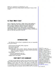
The spectral element method offers two paths to convergence: algebraic through (global) element refinement (h-refinement) and exponential (when the solution is suitably smooth) through increasing the intraelement interpolation order (p-refinement). Basic discretization The spectral element solution proceeds by first fitting the flow domain with an unstructured grid made up of elements. The solution within each element is approximated with a high-degree polynomial. Minimizing the residual resulting from this approximation determines the polynomial’s coefficients and enforces the physical laws governing the fluid motion. This discretization step turns partial differential equations into coupled sets of ordinary differential equations that we can integrate in time using a suitable time-integration procedure. The spectral element method’s distinguishing feature is its choice of collocation points in each element—that is, the points where the solution is interpolated. The collocation points form a mini, unevenly spaced structured mesh in each element (see Figure 1). In fact, the grid spacing decreases toward the element’s boundary. The point clustering serves a dual purpose: eliminating the accuracy loss that occurs near the edges when using high-order polynomial interpolation and providing the quadrature points needed to evaluate numerically and accurately the integrals arising from the residual minimization. Usually, the interpolation and quadrature points are the Gauss-Lobatto roots of Legendre polynomials. The dual roles of interpolation and quadrature translate to tremendous computational efficiency; particularly, they simplify explicit time-stepping procedures to the level of finite-difference techniques. Two options are available to control and reduce errors in spectral element calculations: the number and sizes of elements and the interpolation order. The optimal resource allocation between the global and local grids—the h- versus p-type discretization—is problem dependent. We compute smooth solutions in regular geometries most efficiently with few elements and high-order interpolation. Complicated geometries and localized flow features, such as fronts and jets, require using more elements and lower-order interpolation. Seventh- or eighth-order interpolations are common in practical applications because they seem to be a good compromise between accuracy and computational efficiency.2 The geometry and

SEPTEMBER/OCTOBER 2002

flow complexity then determine the number of elements needed. The current generation of spectral element geophyiscal models uses a static grid and a uniform interpolation order. This static choice is unlikely to be always optimal across the highly variable flow regimes in the ocean and atmosphere. Because the best h-p balance is time and space dependent, some form of grid adaptation is necessary to keep this balance optimal. Researchers have attempted to address the space dependency issue by reformulating the algorithm to use different interpolation orders in different regions.3,4 However, dynamic grid adaptation has not yet received the attention it deserves; this issue should gain prominence as atmospheric and oceanic spectral element-based models mature. In a traditional spectral element formulation, a continuity requirement connects and couples the computations in neighboring elements. (This requirement can be bypassed when using either a nonconforming or a discontinuous Galerkin formulation.) In practice, satisfying this requirement is easy; the sole restriction is that a single value of the solution be used on either side of the shared edge. Thus, in contrast to higher-order finite-difference methods, only edge points exchange information across elements. This last property makes the spectral element method ideally suited for parallel computations. Parallel scalability From a parallel computation viewpoint, we can classify the spectral element method as a coarsegrained algorithm, because we must perform dense local computations before requiring sparse interelement communication. In two dimensions, the computational cost grows like KN 3, where K is the number of elements on each processor and N – 1 is the degree of the interpolation polynomial. The communication cost grows like K 1/2N. The ratio of the computational time between the serial and parallel codes measures the speedup. We can estimate it as S = P/(1 + K–1/2N–2), where P is the number of processors. K–1/2N–2 measures the overhead the parallel computations (excluding latency) incur and ideally should be zero for perfect scalability. Our back-of-the-envelope estimate shows that the overhead decreases quadratically with the degree of the interpolation polynomial and as a weak power of the number of elements in each processor. The formula also shows that the communication cost increases only linearly with the method’s order, whereas its com-

43

A Short History of Spectral Elements in Geophysics Anthony Patera and his collaborators initiated the development and application of the spectral element method for engineering fluid flow problems .1–3 For geophysical flows, Hong Ma was the first to present a spectral element model to solve 2D shallow water equations.4 Further development continued at Rutgers University under John P. Boyd and Dale B. Haidvogel. The effort at Rutgers focused primarily on developing a model for realistic oceanic simulations.5,6 This model has been used in various applications, including an investigation of the global long period ties in the ocean and the transient adjustment of the abyssal circulation in the East Mediterranean Sea.7 Mark Taylor produced an atmospheric version of the model capable of handling the polar singularity.8 Testing it on a suite of standard problems established its good properties in the atmospheric context. Taylor then extended the model to three dimensions; it is undergoing further development at the National Center for Atmospheric Research.9 On the oceanic side, and to the best of our knowledge, the spectral element ocean model (SEOM)6,10 is the only 3D oceanic model currently available. It solves the hydrostatic primitive equations traditional in atmospheric and oceanic modeling. To date, we have applied 3D SEOM primarily to investigate oceanic processes in idealized settings—for example, the interaction of tidal currents with a submarine canyon. The main text focuses primarily on the oceanic model, although much of the description can apply to the atmospheric model. Interest in spectral-element based geophysical models has increased in recent years, as the number of models currently under development demonstrates; we cite particularly the work of Francis Giraldo and his colleagues,11 and Frederic Dupont.12

References 1. Y. Maday and A.T. Patera, “Spectral Element Methods for the Incompressible Navier-Stokes Equations,” State of the Arts Surveys in Computational Mechanics, A.K. Noor, ed., Am. Soc. of Mechanical Engineers, New York, 1988. 2. E.M. Ronquist, “Optimal Spectral Element Methods for the Unsteady Three-Dimensional Incompressible Navier-Stokes Equations,” doctoral thesis, Massachusetts Inst. of Technology, Cambridge, Mass., 1988. 3. G. Karniadakis and S.J. Sherwin, Spectral/hp Element Methods for CFD, Oxford Univ. Press, New York, 1999. 4. H. Ma, “A Spectral Element Basin Model for the Shallow Water Equations,” J. Computational Physics, vol. 109, 1993, pp. 133–149. 5. M. Iskandarani, D.B. Haidvogel, and J.P. Boyd, “A Staggered Spectral Element Model with Application to the Oceanic Shallow Water Equations,” Int’l J. Numerical Methods in Fluids, vol. 20, 1995, pp. 393–414. 6. D.B. Haidvogel and A. Beckmann, Numercial Ocean Circulation Modeling, Imperial College Press, London, 1999. 7. E.N. Curchitser, D.B. Haidvogel, and M. Iskandarani, “On the Transient Adjustment of a Midlatitude Abyssal Ocean Basin with Realistic Geometry and Bathymetry,” J. Physical Oceanography, vol. 31, no. 3, 2001, pp. 725–745. 8. M. Taylor, J. Tribbia, and M. Iskandarani, “The Spectral Element Method for the Shallow Water Equations on the Sphere,” J. Computational Physics, vol. 130, no. 1, Jan. 1997, pp. 92–108. 9. R. D. Loft, S.J. Thomas, and J.M. Dennis, “Terascale Spectral Element Dynamical Core for Atmospheric General Circulation Models,” submitted to J. SuperComputing, 2001. 10. M. Iskandarani, D.B. Haidvogel, and J. Levin, “A Three-Dimensional Spectral Element Model for the Solution of the Hydrostatic Primitive Equations,” submitted to J. Computational Physics, 2002. 11. F.X. Giraldo, J.S. Hesthaven, and T. Warburton, “A Nodal Discontinuous Galerkin Method for the Spherical Shallow Water Equations,” in review, J. Computational Physics. 12. F. Dupont, Comparison of Numerical Methods for Modeling Ocean Circulation in Basins with Irregular Coasts, doctoral thesis, McGill Univ., Canada, 2001.

putational cost increases cubically, yielding a quadratic ratio between the two. This ratio gives the method its coarse-grain character. In contrast, high-order finite-difference methods show a quadratic increase of the communication cost with the order, because the number of halo points that must pass between processors increases. Geometric flexibility in ocean modeling Figure 1 shows an example of a spectral element ocean model grid covering the majority of the global ocean. In SEOM, the elements are quadrilaterals. Grids based on triangular elements are also possible.3,5 The grid’s unstructured nature is clear from the irregular adjacency patterns between elements, and it gives the method its great

44

geometrical flexibility. It permits a better geometrical description of the complex ocean basins, easily accommodates spatially variable resolution to represent regionally localized, fine-scale processes (such as western boundary currents like the Gulf Stream and Kuroshio), and therefore enables multiscale simulations in the framework of a single model. The grid in Figure 1 has finer resolution in the North Pacific Ocean, particularly in its coastal and equatorial wave guides, which are essential pathways of El Niño signals. These regions are tiled with small elements whose average size is approximately 100 km. The element size is larger outside the North Pacific Basin. The North Atlantic and Indian oceans are tiled at reduced resolution to simulate, albeit crudely, remote oceanic influences and to avoid problems with open boundaries. Scientists are using simi-


Figure 1. Elemental partition of the global ocean as seen from the eastern and western equatorial Pacific. The inset shows the master element in the computational plane. Circles mark the interpolation points.

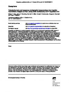
larly designed multiscale grids to explore how climate variability impacts regional ecosystems.6 An important constraint on coupled climate models today, particularly on their oceanic component, is that affordable spatial resolution typically limits or excludes the dominant energycontaining scales of motion (boundary currents and mesoscale eddies). Multiscale models such as SEOM offer the prospect of enhancing these processes’ resolution, at least in limited regions. Figure 2 shows an example of a multiscale simulation conducted with SEOM’s shallow water version. The grid resolution is coarse away from the Gulf Stream region and very fine along the US eastern coast. The model successfully captures the Gulf Stream’s strong mesoscale meandering using a global telescoping grid whose elements’ sizes range from 100 to 1,000 km.


Three-dimensional considerations in SEOM To date, most spectral element-based oceanic models are 2D (see the sidebar). To the best of our knowledge, SEOM is the only 3D spectral element ocean model designed for solving the hydrostatic primitive equations.7,8 Here, we discuss some issues pertaining to the vertical representation of the solution. Given the large difference between the vertical- and horizontal-length scales in the ocean (and the atmosphere), solution and geometry discretization have unusual importance. Representing the water column’s vertical structure is particularly problematic, because it involves complicated (tall and steep) marine topography covering a wide range of length scales. Three common choices of vertical coordinate are

45

Figure 2. Simulation of the wind-driven circulation in the Atlantic Basin using a telescoping global grid. We used small elements in the Gulf Stream region and sixth-degree polynomials to interpolate the velocity. The contours represent the interface height of the wind-driven layers. The Gulf Stream’s detachment occurs at Cape Hatteras. The two panels depict the pinching and subsequent propagation of cold core eddies.

• Z-layer coordinates, where a stack of horizontal slabs interrupted by topography discretizes the vertical direction. • Layered models, where the water column is divided into isopycnal (equal density) layers. • Terrain-following coordinates, where the computational surfaces follow the sloping bathymetry. For a spectral element model, the z-level approach is a poor choice; the topography’s firstorder representation is inconsistent with highorder algorithms. The layered discretization is also currently impractical, because it requires robust numerical schemes that can handle discontinuous solutions without noise generation. These schemes are available for low-order methods but not high-order ones, where they continue to be a topic of active research. Terrain-following discretizations can accurately represent topographic processes, provided the underlying bathymetry is well resolved on the computational mesh. Because it is in this limit that these higher-order methods best apply, terrain-following coordinates are the obvious choice for geophysical spectral element methods. SEOM’s vertical discretization is based on a full spectral element formulation, where the elements are 3D hexahedra that follow the bottom topography. Given the complicated bathymetry of ocean basins and the lack of appro-

46

priate 3D grid generation software, the elemental partitioning in the vertical is restricted to a uniform number of vertical elements. The 3D spectral element grid can thus be produced by stacking vertically and conformally 2D grids. This restriction is not severe; we can still distribute vertical resolution according to a priori considerations. Figure 3 shows the spectral element grid’s vertical structure (used in a study of submarine canyons).9 Unresolved issues Several computational issues remain unresolved in applying finite-element methods to geophysical flows, including • Local conservation • Effective subgrid-scale parameterizations to rapidly damp small-scale noise while preserving large-scale features • Availability of robust advection schemes that can handle poorly resolved flow features without generating noisy solutions • Water mass property preservation on decadal and longer timescales • Grid generation and adaptivity The resolution of these issues in the traditional spectral element formulation context is unclear. Fortunately, the discontinuous Galerkin


0 –2 –4 –6 –4 –8 –10 –12 35

40

45

50

55

60

method provides a powerful new paradigm for modeling nearly inviscid fluid flows.3,10 The DGM’s distinguishing feature is that the numerical solution can be discontinuous across element boundaries. The method localizes computations even more than the continuous formulation. Communication between elements occurs through fluxes exchanged across element edges and can be biased to favor information coming from upstream. Furthermore, conservation is locally satisfied because fluxes are unique along edges. Thus, the DGM possesses the two desirable properties of upstream flux bias and local conservation. Additionally, because the solution interpolation is discontinuous, locally adaptive gridding is immensely simplified. We have successfully reformulated the portions of 3D SEOM responsible for temperature and salt advection using the DGM. The new code has demonstrated improved robustness in several process-oriented test problems. We are currently working on testing this new formulation’s performance on realistic basin-scale problems.

I

n addition to reformulating basic numerical algorithms, we are also developing the physical submodels necessary for successful climate simulations. We mention particularly the parametrization needed to represent the vigorous vertical mixing that occurs in the ocean (within the surface mixed layer, for example). Despite its localized nature, this mixing is pivotal in establishing the upper ocean’s vertical structure and maintaining the deeper thermohaline circulation. The turbulent flows lead-


65

70

75

80

85

90

ing to this mixing are typically subgrid scale, and their net effects must therefore be parameterized. We have successfully embedded a mixing parameterization based on the formulation of Bill Large and his colleagues.11 A submodel for the growth, retreat, and movement of sea ice is also essential to represent climate interactions in the polar regions; we are working on coupling a sea-ice model to our SEOM code. The primary challenge there is representing the often discontinuous ice dynamics in the high-order SEOM framework.

Figure 3. A vertical slice of a 3D spectral element grid showing the elemental partition.6 The elements are refined near the bottom to improve the resolution of near-bed dynamics. The vertical and horizontal scales are in centimeters.

Acknowledgments Grants from the US Office of Naval Research (Ocean Modeling and Prediction), the National Science Foundation (Advanced Computational Methods, Physical Oceanography), and the Goddard Institute for Space Studies have supported the spectral element model’s development and application. The National Center for Atmospheric Research, the National Center for Supercomputing Applications, the Arctic Region Supercomputing Center, and the NOAA Forecast Systems Laboratory provided the resources for applying SEOM to regional climate studies.

References 1. J. Willebrand and D.B. Haidvogel, “Numerical Ocean Circulation Modeling: Present Status and Future Direction,” Ocean Circulation and Climate, Academic Press, New York, 2001, pp. 547–556.

47

2. M. Taylor, J. Tribbia, and M. Iskandarani, “The Spectral Element Method for the Shallow Water Equations on the Sphere,” J. Computational Physics, vol. 130, no. 1, Jan. 1997, pp. 92–108. 3. G.E. Karniadakis and S.J. Sherwin, Spectral/hp Element Methods for CFD, Oxford Univ. Press, New York, 1999.

Massachusetts Institute of Technology. Contact him at the Institute of Marine and Coastal Sciences, Rutgers University, 71 Dudley Rd, New Brunswick NJ, 08901; [email protected].

4. J. Levin, M. Iskandari, and D.B. Haidvogel, “A Nonconforming Spectral Element Ocean Model,” Int’l J. Numerical Methods in Fluids, vol. 34, no. 6, 2000, pp. 495–525. 5. B. Wingate and J.P. Boyd, “Spectral Element Methods on Triangles for Geophysical Fluid Dynamics Problems,” Proc. 3rd Int’l Conf. Spectral and High-Order Methods, Houston J. Math., Houston, 1996, pp. 305–314. 6. A.J. Hermann et al., “A Coupled Global/Regional Circulation Model for Ecosystem Studies in the Coastal Gulf of Alaska,” Progress in Oceanography, vol. 35, nos. 2–4, pp. 235–255. 7. D.B. Haidvogel and A. Beckmann, Numercial Ocean Circulation Modeling, Imperial College Press, London, 1999. 8. M. Iskandarani, D.B. Haidvogel, and J. Levin, “A Three-Dimensional Spectral Element Model for the Solution of the Hydrostatic Primitive Equations,” submitted to J. Computational Physics, 2002. 9. N. Perenne, Dale B. Haidvogel, and D.L. Boyer, “Laboratory-Numerical Model Comparisons of Flow Over a Coastal Canyon,” J. Atmospheric and Oceanographic Technology, vol. 18, no. 2, 2000, pp. 235–255. 10. B. Cockburn, “An Introduction to the Discontinuous Galerkin Method for Convection Dominated Flows,” Advanced Numerical Approximation of Nonlinear Hyperbolic Equations, A. Quarteroni, ed., Springer-Verlag, New York, 1998, pp. 151–268. 11. W.G. Large, J.C. McWilliams, and S.C. Doney, “Oceanic Vertical Mixing: A Review and a Model with a Nonlocal Boundary Layer Parameterization,” Reviews in Geophysics, vol. 32, 1994, pp. 363–403.

Mohamed Iskandarani is an associate research professor in the Department of Meteorology and Physical Oceanograpy at the University of Miami. His research interests include geophysical and computational fluid dynamics, hydrodynamics, and coastal engineering. He has a BS in civil engineering from the American University of Beirut and an MSc and PhD in civil and environmental engineering from Cornell University. Contact him at the Rosenstiel School of Marine and Atmospheric Science, 4600 Rickenbacker Causeway MSC320, Miami, FL 33149-1098; miskandarani@rsmas. miami.edu.

Dale B. Haidvogel is a professor at the Institute of Marine and Coastal Sciences at Rutgers University. His research interests include coastal ocean processes and prediction, regional climate studies, and coupled physical and biological modeling. He has a BS in physical sciences and a PhD in physical oceanography from the

48

Julia C. Levin is an assistant research professor at Rutgers University. Her research interests include ocean modeling, computational fluid dynamics and numerical analysis, large-scale scientific computing, and parallel numerical methods. She has a BS in applied mathematics from Moscow Oil and Gas Academy and an MS and PhD from Columbia University. Contact her at the Institute of Marine and Coastal Sciences, Rutgers University, 71 Dudley Rd, New Brunswick NJ, 08901; [email protected].

Enrique Curchitser is an associate research scientist at the Lamont-Doherty Earth Observatory at Columbia University. His research interests include large-scale ocean circulation, sea-ice ocean interactions, numerical modeling, and parallel computational methods. He has a BS and MS in mechanical and aerospace engineering and a PhD in physical oceanography from Rutgers University. Contact him at the Lamont-Doherty Earth Observatory of Columbia University, 61 Route 9W, Palisades, NY 10964; [email protected].

Christopher A. Edwards is an assistant professor in the Ocean Sciences department at the University of California, Santa Cruz. His research interests include geophysical fluid dynamics, ecosystem dynamics, and ocean observing systems. He has a BS in physics from Haverford College and a PhD in physical oceanography from the Massachusetts Institute of Technology and the Woods Hole Oceanographic Institution. Contact him at the Ocean Sciences Department, University of California, Santa Cruz, CA 95064; christopher. [email protected].

For more information on this or any other computing topic, please visit our Digital Library at http://computer. org/publications/dlib.
