Feature Selection Using a Piecewise Linear Network

IEEE TRANSACTIONS ON NEURAL NETWORKS, VOL. 17, NO. 5, SEPTEMBER 2006

1101

Feature Selection Using a Piecewise Linear Network Jiang Li, Member, IEEE, Michael T. Manry, Pramod L. Narasimha, Student Member, IEEE, and Changhua Yu

Abstract—We present an efficient feature selection algorithm for the general regression problem, which utilizes a piecewise linear orthonormal least squares (OLS) procedure. The algorithm 1) determines an appropriate piecewise linear network (PLN) model for the given data set, 2) applies the OLS procedure to the PLN model, and 3) searches for useful feature subsets using a floating search algorithm. The floating search prevents the “nesting effect.” The proposed algorithm is computationally very efficient because only one data pass is required. Several examples are given to demonstrate the effectiveness of the proposed algorithm. Index Terms—Feature selection, regression, piecewise linear network (PLN), orthonormal least squares (OLS), floating search.

I. INTRODUCTION EATURE or input variable selection plays a very important role in many multivariate modeling problems, where the best subset of features is not known. We focus on feature selection for regression tasks in this paper. Irrelevant features can lead to several problems when nonlinear networks are used for modeling [1]: 1) Training an unnecessarily large network requires more computational resources and memory, 2) high dimensional data may have the curse of dimensionality problem if the available data is limited, and 3) training algorithms for large networks can also have convergence difficulties and poor generalization. The goal of feature selection is to generate a compact subset of features that leads to an accurate model based on the limited amount of data. Feature selection methods usually consist of three steps: Feature evaluation, feature subset search, and feature subset validation (stopping criterion). Feature evaluation estimates the fitness of features based on a user chosen criterion. Feature subset search attempts to find a combination of the features that maximizes the fitness criterion. Feature subset validation is used to determine the number of features that is sufficient for the given data. Feature evaluation for regression tasks may be divided into filter and wrapper approaches in the same way as its counterpart in classification [2] and [3]. A filter approach estimates the

F

Manuscript received May 7, 2005; revised January 31, 2006. This work was supported by the Advanced Technology Program of the state of Texas under Grant 003656-0129-2001. J. Li was with the Department of Electrical Engineering, University of Texas at Arlington, Arlington, TX 76019 USA. He is now with the Department of Radiology, Warren G. Magnuson Clinical Center, National Institute of Health, Bethesda, MD 20892 USA (e-mail: [email protected]). M. T. Manry and P. L. Narasimha are with the Department of Electrical Engineering, University of Texas at Arlington, Arlington, TX 76019 USA (e-mail: [email protected]). C. Yu was with the Department of Electrical Engineering, University of Texas at Arlington, Arlington, TX 76019 USA. He is now with Fastvdo LLC, Columbia, MD 21046 USA. Color versions of Figs. 1–4 are available online at http://ieeexplore.ieee.org. Digital Object Identifier 10.1109/TNN.2006.877531

fitness values for features without any actual model assumed between outputs and inputs of the data. A feature can be selected or discarded based upon some predefined criteria such as mutual information [4], [5], principal component analysis [6], [7], independent component analysis [1], [8], class separability measure [9], [10], or variable ranking [11]. Filter approaches have the advantage of computational efficiency but do not take into account the biases of regression models. On the other hand, wrapper approaches calculate the fitness of a feature subset by actually implementing a full regression model. A wrapper approach usually selects a model, optimizes the parameters, measures the fitness of the features and selects the feature subset which has the largest fitness value. The neural network paradigms most related to the wrapper approach are pruning methods [12]–[14], growing methods [15], [16], and hybrid methods [17], [18]. Usually, wrapper approaches give better results than filter approaches, because both the modeling and selection procedures are based on similar models [2]. However, wrapper approaches have higher computational complexity since evaluation of fitness values require passes through the data. Note that feature selection algorithms are not restricted to selecting input subsets. They can be extended to hidden unit pruning in neural networks [19]. There is another particular feature selection methodology that is neither a filter nor a wrapper method, which is based on a trained neural network [20]–[22]. Here, the fitness of one feature is calculated from parameters of the trained network. For example, one can evaluate the summation of all the weight magnitudes connected to an input [23]. However, the summation of weight magnitudes is fixed once the network is trained, so it does not reflect the dynamical interaction among the features: Adding one correlated feature into a set of features has a big effect on the magnitudes of the other weights in the network. Search algorithms used in feature selection are often growing or pruning methods. The former approach adds features to the current feature subset and is sometimes called a “bottom-up” search. The latter approach removes features from the current feature subset until a satisfactory result is obtained, and is sometimes called a “top-down” search. However, both approaches suffer from the so-called “nesting effect.” In the top-down search, a discarded feature cannot be reselected while in the bottom-up search a feature cannot be discarded once selected [24]. Since the fitness of a set of features depends upon correlations among them, a feature with a high fitness value does not necessarily belong to the optimal subset. From the literature of feature selection for classification, we know that the optimal search algorithm is the branch and bound [25], which requires a monotonic criterion function. Although branch and bound is very efficient compared to the exhaustive search, it still becomes impractical for data sets with more than about 30 features. Attempts to prevent the nesting effect and to attain algorithm efficiency include the plus-l-minus-r

1045-9227/$20.00 © 2006 IEEE

1102


search method [26] and the floating search algorithm [24]. The drawback of the algorithm is that there is no theoretical way of predicting the values of and to achieve the best feature subset. The floating search algorithm is an excellent tradeoff between the nesting effect and computational efficiency, and there are no parameters to be determined. Though the floating search was originally proposed for classification tasks, it is readily extended to regression applications if the fitness criterion is appropriately formulated. To perform feature subset validation, the available data may be further divided into training and validation sets. The search procedure is performed on the training set and the search stops when the stopping criterion, such as the significance test of the validation errors on the validation set, is satisfied [3]. If the data size is sufficiently large with respect to the complexity of the regression model, Fisher tests can be used. Otherwise, a leave-one-out method may be a good alternative [27]. Stoppiglia et al. [28] proposed to append to the set of candidate features a “probe” feature, which is a random variable. All features that are ranked below the probe feature should be discarded. They proved that this is closely related to the Fisher test. Regularization or D-optimality [29]–[31] have also been proposed for determining the number of features that should be included in the final model. The orthonormal least squares (OLS) [32] procedure has been applied to construct a sparse kernel regression method [33], [34] [29], [30]. It has also been combined with a lattice partitioning piecewise linear network (PLN) for construction of neurofuzzy networks [31]. In this paper, we develop an efficient wrapper type of feature selection algorithm for regression utilizing a modified Gram–Schmidt OLS procedure. The floating search method is extended to the regression case to prevent the nesting effect, and we evaluate the fitness values of feature subsets based upon the OLS procedure in an PLN. The paper is organized as follows. In Section II, we review the OLS procedure for forward selection in a linear regression network. In Section III, an overview of the floating search algorithm is presented and is applied to feature selection for the linear network presented in Section II. The proposed piecewise linear orthonormal floating search algorithm is given in Section IV. Section V discusses connections between the proposed algorithm and other related algorithms. The predicted mean square error (MSE) for an equivalent multilayer perceptron (MLP) is described in Section VI. Numerical examples are given in Section VII, and we conclude this paper in Section VIII. II. OLS PROCEDURE FOR FORWARD SELECTION In this section, we review forward selection in a linear regression network. An efficient implementation was given in terms of OLS and the modified Gram–Schmidt algorithm [32]. OLS is the basis for our proposed algorithm, and the modified Gram–Schmidt algorithm makes OLS very efficient.

the multiple-input–multiple-output (MIMO) regression model of the form (1) (2) where is the desired value of is the error between the th output for the th pattern, and and the model output . Here, we let to is the model weight from the handle output thresholds. th feature to the th output, is the th feature or regressor, is the total number of candidate features, and the number of outputs. Substituting (1) into (2) yields (3) By defining

(4)

(5)

(6) (7)

the regression model (3) now can be written in the matrix form (8) The task of feature selection for regression is to select the most significant subset from the set of available features. The OLS procedure selects a set of features to form a set of or, in a forward manner. thonormal bases , Suppose can be decomposed as (9) where

A. Orthonormal Linear System , where the input vector Given a set of data pairs and the desired output vector , consider

(10)

LI et al.: FEATURE SELECTION USING A PIECEWISE LINEAR NETWORK

1103

and

B. Forward OLS Procedure (11)

Here, in [32]

, where denotes the identity matrix. Note that was decomposed to an orthogonal basis as

(12) where

with

(13) where

is the square of the length of , we get

The forward OLS procedure has been successfully applied to construct kernel regression models and neurofuzzy systems [29]–[31], [33], [34]. System (16) consists of subsystems and can be denoted as follows:

(19) is where the weight matrix connecting to the th output, and . Multiplying (19) by its transpose and time averaging, the following is easily derived:

. Defining

(20) (14) and (15) In other words, in order to get the orthonormal basis , the th is normalized by the length row in the transformation matrix . of The regression model of (8) now becomes

(16) denotes the weights for the orthonormal system. The where least square solution for (16) is

(17) which is projection of the desired output onto the othonormal bases. The weights for the original system can be easily obtained as

(18) If none of the features are linearly dependent on the others, the decomposition (9) and the transformation (18) are always possible. The decomposition procedure is done using the algorithm given in Appendix I in which the data is accessed only once. The orthonormal weights are obtained based only on the autocorrelation and cross-correlation matrices. Once these matrices are calculated through one data pass, the orthonormal procedure only utilizes these matrices, whose sizes are usually much smaller than those of the original data. Therefore, a very efficient algorithm can be implemented.

The variance or energy for the th output contains two parts , the variance explained by the features, and , the unexplained variance for the th output. The error reduction ratio for the th output due to the th feature is defined as

(21) The most significant features are forward selected according to . At the first step, we calculate for the value of the th feature treating it as the first feature to be orthonormalis obtained using (21). The feature is selected ized; then, if it produces the largest value of . At the second step, the aforementioned steps are repeated for the remaining features. For multiple output systems, one could apply the forward selection procedure to each output separately and obtain a different feature subset for each output system. This is necessary if each subsystem has different dynamics (see [31]). However, if the multiple output systems have similar dynamics, the selected subset features for each output may not differ much from one to another. We can then make a tradeoff between the complexity and the accuracy as follows. We keep the same feature subset for each output, and the error reduction ratio (21) for the th feature is modified as

(22) which is the total error reduction ratio of the th feature for all of the output systems. The feature is selected if it has the largest in the forward selection procedure. Note that the denominator in (21) is a constant for all features; we can just simply ignore it.

1104


III. FLOATING FEATURE SEARCH METHOD FOR REGRESSION The drawback of the forward selection procedure in Section II-B is the nesting effect which means that a feature cannot be discarded once selected. In this section, we review the floating search method for feature selection, and again in the linear network. from It is well known that when selecting a subset of features , the optimal solution involves the given evaluating all possible subsets of size . It is obvious that the number of combinations needing to be evaluated increases or . Though the branch and bound exponentially with [25] algorithm reduces search time significantly, it is still not or . For these reasons, feasible for even a mild value of some tradeoffs between the optimality and efficiency of the algorithm have been made. Pudil et al. [24] proposed a floating search method for classification, which is a near-optimal solution that significantly reduces the computational load. The floating search method consists of forward and backward floating selection. Both of them have similar performances, but the forward one is computationally faster. We, therefore, extended the forward floating search algorithm for regression in this paper. In order to describe the floating search algorithm, we first introduce the following definitions. be a set of Let features from of available features. is Definition 1: The individual fitness of one feature

(23) which is the total variance explained for all outputs due to the th feature. This is a general measure of the fitness value of one feain the orthonormal ture regardless of the selection order of procedure. is Definition 2: The total fitness of a set of features measured as

(24) which is the total variance explained for all the outputs due to all features in . Here, the features in are made orthonormal to each other according to the order as they are selected. in is Definition 3: The fitness of defined as

(25) is equivalent to the general fitness In other words, value of calculated using (23), where is the last feature that is made orthonormal to the other features in . in This measure is used to identify which feature in the selected feature pool is the least significant one. The least significant

can be identified in the following procedure: For feature in , where , let be the last feature each ; the fitness to be made orthonormal to other features in of is then calculated as (25). This procedure is repeated times; is identified as the least significant feature in if

(26) Definition 4: The fitness of , is

with respect to

, where

(27) The goal of this measure is to identify which feature in the remaining feature pool is the most significant one. The most sigis identified as follows: For each nificant feature in , make it orthonormal to and calfeature as (23). This process is repeated culate the fitness value of times and the most significant feature with respect to is identified as if

(28) Definition 1 is a general measure that constructs basis for the other three definitions. Definition 2 is a measure of the stopping criterion for the continuation of the conditional deletion. Definition 3 is used in the conditional deletion, and Definition 4 is used in the adding one feature step in the forward floating search algorithm. See Appendix II for the details of the forward floating search algorithm. IV. PIECEWISE LINEAR ORTHONORMAL FLOATING SEARCH ALGORITHM We have introduced the floating search algorithm for a linear system. However, feature selection for a nonlinear system should be based on a nonlinear model. In this section, we extend the floating search algorithm for linear regression to the piecewise linear regression case. Some important issues about this algorithm are also addressed. A. Piecewise Linear Orthonormal System It has been shown that a PLN model can approximate a nonlinear system adequately [35]. A PLN often employs a clustering method to partition the feature space into a hierarchy of regions (or clusters), where simple hyperplanes are fitted to the local data. Thus local linear models construct local approximations to nonlinear mappings. As the number of training patterns tends to infinity, partition based estimates of the regression function converge to the true function and the MSE of mapping converges to that corresponding to Bayes rules [36], [37]. Thus PLNs are consistent nonparametric estimators, and feature selection based on the PLN model should be more accurate. Some


1105

successful applications of these kinds of local processors can be found in [35] and [38]–[41]. The regression model (8) for the PLN can be rewritten as

(29) where the superscript denotes to which the input vector is assigned. For each cluster, we apply the modified Gram–Schmidt procedure to the data belonging to that cluster, yielding

(30) If the output systems have similar dynamics, we could use the same feature space partition for all the systems. Suppose we clusters, the floating initially partition the feature space into search algorithm based on the PLN model is defined the same as in Section III except that the fitness definitions (23) through (24) should be modified as follows. is 1) The individual fitness of one feature

(31) 2) The total fitness of

is

(32) There are two important issues to be noted for this algorithm. First, we need to determine an appropriate number of clusters for partitioning the feature space. Second, in the algorithm the autocorrelation and cross-correlation matrices for the clusters are calculated only once and are used in the whole search procedure without being recalculated. By using one data pass we significantly reduce the computational load. However, using the same matrices for different size feature subsets implies that we keep the partition unchanged while the feature subset size changes. This could have some deleterious effects on the selection result, and Section IV-B discusses these two issues. B. Number of Clusters and Partition of Feature Space Determining the number of clusters in a PLN for a given set of data is a model validation or model selection problem. Model selection is a difficult task because it is not possible just simply to choose the model that fits the data best: More complex models always fit data better, but bad generalizations often result. Bayesian methods [42] employ “Occam’s Razor” to penalize unnecessarily complex models in the selection procedure. Growing methods [15], [43], [16], pruning methods [44], [45], [12]–[14], Akaike’s information criterion [46], and kernel principal component analysis (kernel-PCA) [47] also have been investigated for model selection. In this paper, we utilized a cross-

validation (CV) method to determine an appropriate number of PLN clusters for a given data set. We selected a model based on a curve produced in the CV procedure. Initially, the feature space of the training data set is partitioned into a large number of clusters using a self-organizing-map (SOM) [48]. For each cluster, a linear regression model is then designed, and the total unexplained variance (training error) is calculated. The trained PLN model is then applied to the validation data set to get its validation error. Our goal is to find the PLN structure such that its validation error reaches the minimum. A cluster is pruned if its elimination leads to the smallest increase of the training error, and the remaining local linear models are redesigned if necessary. The pruning procedure continues till only one cluster remains. Finally, we produce curves of the training and validation errors versus the number of clusters. We find the minimum value on the validation error curve, and the number of clusters corresponding to the minimum is chosen for the PLN model. C. Effect of the Fixed Feature Space Partition In the feature selection procedure, once the number of clusters is determined, the algorithm uses the SOM to partition the feature space and accumulates the autocorrelation and cross-correlation matrices for each cluster. These matrices remain unchanged during the whole feature search procedure. This implies that the algorithm uses the initial partition, which involves all features, for any feature subspace. The advantage of doing this is that we can significantly reduce the computational load of the algorithm. One could repartition the subfeature space and recalculate the autocorrelation and cross-correlation matrices for each feature subset, which may produce a more accurate estimate of the unexplained variance for the selected features, but this is not feasible for data with a large number of features. However, our approach may produce an optimistic estimate of the unexplained variance, for a small feature subset. D. Algorithm Description Assuming that we have a training data set and a validation data set, we describe the proposed floating-OLS algorithm as follows. 1) Initialize , the number of features that need to be secould be set to a small number in the case lected, as . is large. that 2) Determine the number of clusters for the PLN model using the method described in Section IV-B. 3) Design an -cluster PLN model for the training data, and accumulate autocorrelation and cross-correlation matrices for each of the clusters. 4) Use the piecewise linear orthonormal floating search almost important features from the gorithm to find the available features. • The first two features are selected by the forward OLS procedure, based on the fitness value calculated using (27). • In the conditional deletion and the continuation of the conditional deletion procedures of the floating search algorithm (Appendix II), the fitness value of one feature

1106


in the currently selected feature set is calculated by (25), and the fitness of a set of features is calculated by (32). • The piecewise orthonormal floating search algorithm most significant features are secontinues till the lected. 5) Apply the PLN model on the validation data set to get validation errors for each of the selected feature subset. 6) The feature subset which has the minimum validation error is determined as the final selected feature subset. In the case that multiple subsets have validation errors close to the minimum validation error, the feature subset that has the smallest size but whose validation error is not bigger than 105% of the minimum validation error is chosen as the final selected feature subset. Remarks: 1) in this algorithm, all the searching efforts are handled with autocorrelation and cross-correlation matrices of the PLN model; the original data is not used; 2) a linearly dependent feature will be assigned zero-valued weights, and, therefore, its fitness value is zero; 3) in step 6), we heuristically choose the final selected feature subset based on its validation error, i.e., its validation error is not bigger than 105% of the minimum validation error. Optimal stopping criteria are important for feature selection, but this topic is out of the scope of this paper. Other stopping criteria can be used for the developed algorithm. V. RELATED WORK There are many feature or variable selection algorithms in the literature [3]. In this section, we discuss some connections between the proposed algorithm and previous ones. A. Correlation Criteria The Pearson correlation coefficient between feature is defined as the desired output

and

(33) where denotes the covariance and the variance. This coand if they have efficient is also the cosine between is the been centered. In a linear regression, the square of variance of the th output explained by the th feature. The use can be extended to the case of two-class classification of [49]. For our case, we have used the modified Gram–Schmidt procedure to calculate output variances explained by features in an efficient way. Our method is equivalent to the general correlation criteria between outputs and the decorrelated features, and the PLN was used to handle nonlinear regressions. The interactions among features have also been taken into account in the floating search. Note that our algorithm is readily extended to the classification case.

tures, because the orthogonal procedure can decorrelate features and the features can be selected independently. The criterion he used is the Mahalanobis distance measure [10]

(34) is the mean vector of data samples in class . , and and are the covariance matrices of class and class , respectively. Under the orthogonality condition, the is diagonal and the Mahalanobis distance covariance matrix is easy to calculate. They selected feature subsets by a similar orthogonal forward procedure, where one feature was selected if it had the largest Mahalanobis distance value. They showed that “if correlations between candidate features are trivial, employing orthogonal transform does not make much difference; but orthogonal algorithm provide improvements if severe correlations exist.” Other criteria, including the Bhattacharyya distance and the Chernoff probability measure can be used in the orthogonal procedure as well [9]. Their method belongs to the filter category, where no actual classifier is involved in the selection procedure. The advantages of using an orthogonal process are that it decorrelates the original features so that they can be selected independently. Also, physically meaningless features in the Gram–Schmidt space can be linked back to the same number of variables in the original feature space that makes it suitable for feature selection. However, since the nesting effect results from correlations among features as well as correlations between outputs and features, decorrelation of features does not necessarily solve the nesting effect because it does not take into account the correlations of features with outputs. This phenomena is illustrated in Example 1, where our proposed algorithm correctly solves this problem. where

C. Gram–Schmidt Procedure for Regression The Gram–Schmidt procedure has also been used for regression problems. Stoppiglia et al. [28] uses the sequential orthogonal feature selection for linear regression tasks. If nonlinearity between inputs and outputs exist, Rivals et al. [27] first constructs a polynomial of monomials for up to degree to explain this nonlinear relationship. For example, the polynomial of degree 2 involves a constant term and the monomials: . However, not all the terms are significant for explaining the output . A forward sequential orthogonal selection procedure based on the Gram–Schmidt procedure is then performed to select the most significant polynomials for the final regression model. They handle the nonlinearity between inputs and outputs using high-degree polynomial terms, while in our method the nonlinearity is dealt with using a piecewise linear model.

B. Gram–Schmidt Procedure for Classification

D. Principal Component Regression and Partial Least Square Regression

Mao [9], [10] proposed an orthogonal forward feature selection algorithm using the Gram–Schmidt transformation for classification tasks. The motivation of employing the orthogonal decomposition of features is to alleviate the correlation among fea-

Principal component regression (PCR) and partial least square regression (PLS) are two multivariate regression techniques where the number of observations is small compared to the number of features, or the collinearity among features exists


1107

[50], [51]. In such cases, the ordinary multiple regression is not appropriate because overfitting is highly likely. Both PCR and PLS produce factor score matrix as a linear combination of the original feature set as

A. Pattern Storage of PLN and MLP patterns which is equal A linear network can memorize to the number of parameters used to calculate each output. The multiplied by the pattern storage capacity of the PLN is storage capacity per cluster

(35) (38) where the matrix is called the loading for , and is an orthogonal or orthonormal matrix. After the decomposition, a linear regression from to is performed as (36) where is regression weights for . Once regression model (36) is equivalent to

It is well known that the Volterra filter has a storage capacity which is equal to the number of coefficients associated with one is bounded output. The MLP’s pattern storage capacity above by , where is the total number of free is the number of outputs, and it parameters in the network. has been shown that this bound is fairly tight [55]. Therefore, it can be assumed

is computed, the (39) (37)

where . The columns of are called latent factors of . If the number of extracted latent factors is greater or equal to the rank of the original feature space, both PCR and PLS are equivalent to the ordinary multiple regression. PCR and PLS differ from the way how they extract the latent factors: PCR chooses with the goal to explain as much as possible, but may be not relevant to . It is usually performed by a single value decomposition (SVD) , if is centered. On the other hand, PLS chooses to of explain the variance between and as much as possible, which , if both and are centered. is based on the SVD of Both PCA and PLS are feature extraction methods, where there is no clear physical meaning in the extracted feature space since each latent factors is a linear combination of all the original features. However, feature selection algorithms using the Gram–Schmidt procedure have a clear physical meaning because the orthogonal features are linear combinations of the features that have already been selected, and they are readily transformed back to the original feature space. VI. PREDICTED MSE FOR AN EQUIVALENT MLP nonlinear units in a single hidden layer The MLP with has been established as a universal function approximator [52], [53]. Even though it has been shown that the PLN model can train well, the resulting mapping is discontinuous at the boundaries between adjacent clusters. When a discontinuous mapping is unacceptable, we may use a global network such as the MLP. Chandrasekaran et al. [54] proposed a method for sizing the MLP based on the assumption that a PLN with the same theoretical pattern storage capacity as the MLP will have the same training error. For comparison purposes, we implement an MLP-based feature selection algorithm in this paper. As a heuristic, we choose the number of hidden units in the MLP-based feature selection algorithm according to the concept that its pattern storage capacity should be the same as the PLN model found for that data set.

B. Equivalent MLP Equating (38) and (39) yields (40) This formula helps us to estimate the number of hidden units clusters, and it can be in an MLP equivalent to a PLN with divided into two cases. : When the number of outputs , (40) reduces 1) . to : In this case, overly large MLP networks result 2) when the desired outputs are correlated and many free parameters are redundant. An SVD technique is employed to detect whether outputs can be compressed without significantly degrading the MSE performance. Compressing the outputs, we can predict a smaller, less complex MLP. The after we compress the outputs down resulting MSE is given by to (41) is the th singular value of the desired outputs’ where covariance matrix. VII. SIMULATION STUDIES We compared our proposed algorithm with four other algorithms on an artificial data set having one output and with three algorithms on two real data sets having multiple outputs. In the experiments, we divided each data set into a training set, a validation set, and a testing set. The training and validation sets were used for feature selection. The testing set was used to evaluate the selected feature subsets by the ten-fold CV method, using MLPs trained on the feature subsets. We used the paired test to verify if the testing errors for different feature subsets were significantly different in the CV. In this section, we first introduce four additional feature selection algorithms and then give three examples.

1108


A. Feature Selection Algorithms The algorithms compared include two PLN model-based algorithms, where the OLS procedure is used. The third algorithm is an MLP-based feature selection algorithm, and the fourth algorithm is based on the support vector machine (SVM). 1) Search by Importance: There are many feature selection algorithms that are based on weight magnitudes in a trained network [23]. We implemented such method, which we denote the importance method, based upon the PLN model. We first designed the PLN model for the given data, where the number of clusters was determined by CV as described in Section IV-B. The importance of a feature was calculated as the magnitude summation of the weights from the feature to all outputs among all clusters in the PLN. The selection order of features was based on their importance values, with the most important feature selected first. For each cluster, sets of linear equations were solved for weights, using the conjugate gradient method. Once the feature order was calculated, we made all features orthonormal to each other according to the selection order and calculated the training and validation regression errors for each feature subset. The regression error was defined as the standard MSE. 2) Forward-OLS: The forward-OLS feature selection algorithm is the same as floating-OLS, except that forward-OLS uses the forward OLS search (see Section II-B) based on the PLN model. Both the importance and forward-OLS algorithms search feature subsets based on the training data, and the weights for the orthonormal system are transferred back using (18). Networks using the chosen subsets are then applied to the validation data. Both algorithms use the same method as the floating-OLS algorithm (see Section IV-B) to determine the size of the final selected feature subset. 3) Leray: An MLP-Based Algorithm: Leray and Gallinari [22] proposed an MLP feature selection algorithm, denoted Leray, based on the optimal cell damage (OCD) algorithm [20]. Here, the decision on pruning a weight is made according to a relevance criterion often named the weight saliency. The weight is pruned if it has a low salience. The saliency of the th feature is defined as the saliency summation of all the weights connected to the th feature Saliency

Saliency

(42)

where denotes all possible weights connecting the th feature to either a hidden unit or an output. Using an order two Taylor expansion of the MSE and a diagonal approximation for the Hessian matrix, the saliency of the th feature is defined as Saliency

ization error” method, which estimates the generalization performance on a validation set. Since several subsets may have statistically similar performances, Leray uses the Fisher test to compare each model’s performance with that of the best model. Then it chooses the smallest feature subset whose performance is similar to the best one. For a fair comparison in this paper, we used the same method as the floating-OLS algorithm to determine the final feature subset. We compared the validation MSE of any feature subset with that of the best feature subset, and chose the smallest feature subset whose MSE was not bigger than 105% of that for the best feature subset. We selected this algorithm for comparison because it outperforms many other MLP based algorithms, as reported in [22]. 4) An SVM-Based Algorithm: Bi et al. [56] proposed a dimensionality reduction methodology via sparse SVM to perform variable ranking and selection, and to construct a final nonlinear model for the data. The method exploits the fact that a linear SVM with -norm regularization inherently performs variable selection, and the distribution of the linear model weights provides a mechanism for ranking and interpreting the effects of variables. This algorithm was particularly designed for systems with one output. In such situations, we find a functhat minimizes the regularized tion risk functional [56]

(43) where is a loss function, is the desired output for the th pattern, is a regularization operator, and is called the regularization parameter. In [56], the regularized risk functional is defined as

(44) where . By minimizing in (44), a linear model is , where is a threshold and constructed as . After the linear model is constructed, features are ranked by their weight magnitudes. To reduce the weight variability, the algorithm runs several times and the feature ranking is obtained based on the average weight magnitudes. Three random features are added to the data, and the average of their weight magnitudes is used as a threshold for determining the final selected features. The features whose weight magnitudes are bigger than the threshold are included in the final model. B. Example 1 Toydata: This is an artificial data set which contains six features ( trough ) and one output

Leray prunes one feature at a time, and the MLP is retrained after each deletion. For a stopping criterion, Leray uses a variation of the “selection according to an estimate of the general-

(45) where and

through are uniformly distributed between [0 1], are identical, all other features are independent with


1109

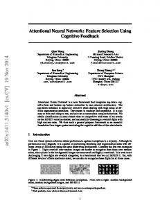
Fig. 1. Regression Errors of PLN on the training and validation toydata sets.

TABLE I AVERAGE WEIGHT MAGNITUDES FOR THE TOYDATA BY THE SVM BASED ALGORITHM

each other, and is white Gausian noise with zero mean and unit variance. Note that is independent of . We generated 10 000 samples for both the training and validation sets, respectively, and 20 000 samples for the testing set. Using the method described in Section IV-B, we first produced PLN training and validation error curves, on the training set and validation set, respectively, and plotted them in Fig. 1. We observed that the number of clusters corresponding to the minimum of the validation error was 21, and the validation error was 1.027. We could say that the 21-cluster PLN is a good model for the nonlinear system because we know that the variance of noise for the output is one. We then ran the three PLN-based algorithms for feature selection, where the PLN had 21 clusters. We also ran the “Leray” algorithm for this data, where the MLP used 20 hidden units, that was calculated using (40). To run the SVM-based algorithm, the training and validation data sets were combined together and were repartitioned randomly in each of ten runs. The average weight magnitudes in the ten runs are shown in Table I. The final model was determined to contain five features with the random feature (the 6th) being excluded. Though the weight magnitudes for the two identical features (the first and the fourth) are different, feature one was, however, not successfully excluded from the final model. The final feature subsets selected by the five algorithms are shown in Table II. We used ten-fold CV on the testing set to evaluate their performances. The equivalent MLPs we used in the

TABLE II TEN-FOLD CV RESULTS ON THE TESTING TOYDATA FOR THE FINAL SELECTED FEATURE SUBSETS

TABLE III TEN-FOLD CV RESULTS ON THE TESTING TOYDATA SET IF FEATURE SUBSET SIZE IS FIXED AT 3

ten-fold CV all had 20 hidden units calculated using (40). Paired tests (at a 95% confidence level) of the CV results showed that the final subsets selected by the five algorithms perform statistically similarly. However, if the feature size is fixed at 3, which is the correct feature size for toydata, Table III shows the testing error of CV results for the five feature subsets selected by the algorithms. The minimum MSE is shown in bold.

1110


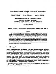
Fig. 2. Ten-fold CV results on the testing toydata set for all size of feature subsets selected by the five algorithms.

Paired -tests were performed between the minimum MSE and the other MSEs. A ‘ ’ sign indicates that the MSE is significantly different from the corresponding minimum MSE at the 95% confidence level. The results clearly show that the feature subset selected by the floating-OLS algorithm is significantly better than those of the other algorithms. The CV MSE is very close to the noise variance, which means that features one, two, and five are adequate to explain most of the variance for the output. For this data set, only the floating-OLS algorithm selected the correct compact feature subset for the regression task. Feature subsets selected by the other algorithms contain unnecessary features, especially the identical feature four and feature one, though all finally selected subsets give statistically similar results. Fig. 2 shows the averages of ten-fold CV MSE results on the testing data set for all size of feature subsets selected by different algorithms, which gives a broad overview for each of the feature selection algorithm. It is clear that the floating-OLS algorithm obtained the best or one of the best results for each case. We will mention that the SVM algorithm was specifically designed for a challenging problem in quantitative structural-activity relationships (QSAR) analysis with the goal of prediction the bioactivity of molecules. Each molecule has many potential features (300–1000) that may be highly correlated with each other or irrelevant to the desired output, and the feature size is much bigger than that of the sample size. There is an assumption that a linear model may be adequate for modeling the data. This may explain why the algorithm failed to identify the correct features for modeling the toydata. The SVM-based algorithm was designed for the one output system only. For a fair comparison, it will not be included in the multiple output data set experiments.

C. Example 2 Twod: This training file is used in the remote sensing task of inverting the surface scattering parameters from an inhomogeneous layer above a homogeneous half space, where both interfaces are randomly rough [57]. The parameters to be inverted are the effective permittivity of the surface, the normalized root-mean-square (rms) height, the normalized surface correlation length, the optical depth, and single scattering albedo of an inhomogeneous irregular layer above a homogeneous half space from backscattering measurements. The data files contain 1238, 530, and 1000 patterns for training, validation, and testing, respectively. The features consist of eight theoretical values of backscattering coefficient parameters at V and H polarization and four incident angles. The outputs were the corresponding values of permittivity, upper surface height, lower surface height, normalized upper surface correlation length, normalized lower surface correlation length, optical depth, and single scattering albedo which had a jointly uniform probability density function (pdf). In this experiment, we tested wether the proposed feature selection algorithm was able to reject noise features. To this end, we added four noise features to the data sets with zero means and standard deviations of 1, 2, 3, and 4, respectively. The training, validation, and testing data sets thus had 12 features (9–12 features were noises) and seven outputs. The number of clusters in the PLN model was determined as 14. We thus ran the three PLN based feature selection algorithms with a 14-cluster PLN model. We also ran the Leray algorithm with 13 hidden units on this data. The number of hidden units was calculated using , because the seven outputs can be compressed (40) with down to one with less than 1% increase in training MSE of an equivalent MLP.


1111

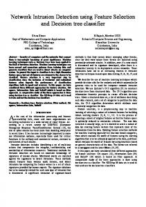
Fig. 3. Ten-fold CV results on the testing twod data set for all size of feature subsets selected by the four algorithms.

TABLE IV TEN-FOLD CV RESULTS ON THE TESTING TWOD DATA SET IF FEATURE SUBSET SIZE IS FIXED AT 6

All four algorithms selected the same feature subset containing all the original features (they are all relevant to the outputs) and successfully rejected the four added noise features. Fig. 3 shows the averages of ten-fold CV MSE results on the testing data set for all size of feature subsets selected by different algorithms. It is clear from Fig. 3 that the floating-OLS algorithm is the best algorithm in this example. It was outperformed only when the feature subset size is 1, where the Leray method was the best algorithm. Though there are other subsets (for example, size 5 and 7), where the floating-OLS did not get the best results, the paired -test showed that the difference between the best algorithm and the floating-OLS algorithm is not significant. For most of the other size feature subsets, the floating-OLS algorithm outperformed the other three algorithms. Table IV shows that it is statistically better than the others if the feature subset size is fixed at 6. D. Example 3 Speech: The speech samples are first pre-emphasized and converted to the frequency domain by taking the discrete

Fourier transform (DFT). Then they are passed through mel filter banks and the inverse DFT is applied to the output to get mel-frequency cepstrum coefficients (MFCC). Each of MFCC(n), MFCC(n)-MFCC(n-1), and MFCC(n)-MFCC(n-2) would have 13 features, which results in a total of 39 features. The desired outputs are likelihoods for the beginning, middle, and ends of 39 phonemes, resulting in 117 outputs. The data files contain 1405, 585, and 2039 patterns for training, validation, and testing, respectively. The number of clusters in the PLN model was determined to be eight. We thus ran the three PLN-based feature selection algorithms based on an eight-cluster PLN model. We also ran the Leray feature selection with an MLP having seven hidden units. Again, the was calculated number of hidden units for the MLP , since the 117 outputs are highly using (40), where correlated and can be compressed down to one with less than 1% increase in training MSE of an equivalent MLP. The sizes of the final selected feature subsets were determined to be 13, 12, 12, and 17 by the importance, forward-OLS, floating-OLS and Leray algorithms, respectively. Table V shows the ten-fold CV MSE and the paired -test results for evaluating the selected feature subsets and the full feature set using equivalent MLPs (all have seven hidden units). The paired test showed that there are no significant differences among the feature subsets selected by the three PLN based algorithms, and the feature subsets selected by the three PLN-based algorithms are statistically better than that by the Leray algorithm and the full feature set. It is clear that using all features in the MLP network for this data are not appropriate, since only 12 out of the 39 features are adequate to model the data. All the PLN-based algorithms selected about 12 features for the final feature subset, and they performed better than the full feature set. The Leray

1112


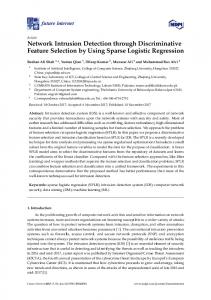
Fig. 4. Ten-fold CV results on the testing speech data set for all size of feature subsets selected by the four algorithms.

TABLE V TEN-FOLD CV RESULTS ON THE TESTING SPEECH DATA SET FOR THE FINAL SELECTED FEATURE SUBSETS

algorithm kept 17 features and performed worse than the other algorithms. Fig. 4 shows the average ten-fold CV MSE results on the testing data set for all feature subset sizes. Since the size of the final feature subsets selected by different algorithms were less than 20, we ran the ten-fold CV only for these relevant feature subsets with a size of less than 20. It is clear that the floating-OLS algorithm is one of the best algorithms compared to others, and the Leray algorithm is the worst. For all the feature subsets, the forward-OLS algorithm is as good as the floating-OLS algorithm which is a sign that a forward-OLS search may be adequate for this highly correlated data. E. Computational Efficiency We compared the computational efficiencies of the four algorithms in terms of the CPU times used in each experiment. Table VI shows the CPU time used by the four algorithms in each experiment. The importance and forward-OLS algorithms used similar amount of CPU time in each experiment. The floating-OLS algorithm needed less than one more second for

TABLE VI CPU TIME NEEDED FOR THE FOUR ALGORITHMS

the first two experiments and 8 s more for the third experiment to complete the search tasks. The Leray algorithm had a much longer computation time than the other three. It needed at least six times more CPU time than the others. For example, in Experiment 2, it cost 104 s of CPU time while the PLN-based algorithms needed about 17 s. VIII. CONCLUSION We have developed a novel feature selection approach for nonlinear regression problems. The algorithm first determines an appropriate PLN model for the given data by cross validation. It then applies the OLS procedure to the PLN. Finally, useful features are chosen by the floating search. The “nesting effect” associated with step forward or step backward search is prevented. The fitness of a feature subset was calculated in the OLS procedure during the selection process based on the autocorrelation and cross-correlation matrices of the original data. This makes the algorithm very efficient because it passes through the data only once to accumulate the correlation matrices. The floating search algorithm always finds the best or one of the best feature subsets, among those selected by the other compared algorithms. The contributions of this paper are two fold: The way nonlinearities are handled and the usage of the floating search


1113

in the OLS procedure. To our knowledge, this is the first time that the floating search has been utilized in an OLS based feature selection algorithm. The examples show that it successfully detects the interaction that among features and that between outputs and features.

Then, obtain

coefficients

(53) Finally, for the are found as

APPENDIX I THE MODIFIED GRAM–SCHMIDT PROCEDURE The normal or modified Gram–Schmidt procedure [32] is a recursive process that requires scalar products between raw basis functions and orthonormal basis functions. The disadvantage of this procedure is that one pass through the training data is required to obtain each new basis function. In the following, a more useful form of the Schmidt process is reviewed, which enables us to express the orthonormal system in terms of autocorrelation elements. Rewrite (9) as

as

th basis function the new

coefficients

(54)

Using (17), the weights for the orthonormal system can be obtained as

(55) where

is the cross-correlation matrix defined as

(46) since is an upper triangular matrix so that triangular. Define

is also upper

(56) Specifically, the weights from the can be expressed as

th basis to the th output

(47) (57) From (46) and (47), the be expressed as

for

th othonormal basis function

can

(48)

If the th feature is linearly dependent with the previous basis functions, we just obtain all zero-valued weights for the th feature. This will eliminate the numerical problem and the linearly dependent feature will not contribute to the explanation of the output variance. Using (18), the weights for the original system can be readily found as

(49)

(58)

, the first basis function is obtained as

where

(50)

The aforementioned process enables us to calculate all of orthonormal basses in terms of the autocorrelation matrix and cross-correlation matrix , which can be obtained by passing through the data only once before the orthonormal process.

and

(51)

is the autocorrelation of and is first found for 2 and

. For values of as

between

(52)

APPENDIX II DESCRIPTION OF THE FLOATING SEARCH ALGORITHM The following is a description of the floating search feature selection algorithm [24]. Initialize , and use the forward and . Suppose we have least square method to form from the available features already selected features . The fitness value and corresponding members for each subset feature have been stored, and we then do as follows.

1114


1) Adding one feature: Find the most significant feature, say , in the set of with respect to using (28), yielding (59) 2) Conditional deletion: Using (26), we find the least signif, in the set of . Then, icant feature, say increment as , and (60) return to step 1). However, if significant feature in the set of from and form a set of

is the least , then delete as (61)

Update

as

(62) and return to step 1). Otherwise, go to step 3). 3) Continuation of the conditional deletion: Find the least sig, in the set . If nificant feature, say , then set , upusing (62), and return to step 1). Otherwise, date delete from to form a new set , . If , set and and set and return to step 1). Otherwise, repeat step 3). ACKNOWLEDGMENT The authors would like to thank Dr. J. Bi for useful discussions and the result she provided for the SVM-based feature selection algorithm. REFERENCES [1] A. D. Back and T. P. Trappenberg, “Selecting inputs for modelling using normalized higher order statistics and independent component analysis,” IEEE Trans. Neural Netw., vol. 12, no. 3, pp. 612–617, May 2001. [2] R. Kohavi and G. John, “Wrappers for feature subset selection,” Artif. Intell., vol. 97, no. 1–2, pp. 273–324, 1997. [3] I. Guyon and A. Elisseeff, “An introduction to variable feature selection,” J. Mach. Learn. Res., vol. 3, pp. 1157–1182, 2003. [4] T. W. S. Chow and D. Huang, “Estimating optimal feature subsets using efficient estimation of high-dimensional mutual information,” IEEE Trans. Neural Netw., vol. 16, no. 1, pp. 213–224, Jan. 2005. [5] V. Sindhwani, S. Rakshit, D. Deodhare, D. Erdogmus, J. Principe, and P. Niyogi, “Feature selection in MLPs and SVMs based on maximum output information,” IEEE Trans. Neural Netw., vol. 15, no. 4, pp. 937–948, Jul. 2004. [6] N. Kambhatla and T. K. Leen, “Dimension reduction by local principal component analysis,” Neural Comput., vol. 9, no. 7, pp. 1493–1516, 1997. [7] J. T. Kwok and I. W. Tsang, “The pre-image problem in kernel methods,” IEEE Trans. Neural Netw., vol. 15, no. 6, pp. 1517–1525, Nov. 2004.

[8] M. D. Plumbley and E. Oja, “A nonnegative PCA algorithm for independent component analysis,” IEEE Trans. Neural Netw., vol. 15, no. 1, pp. 66–76, Jan. 2004. [9] K. Z. Mao, “Fast orthogonal forward selection algorithm for feature subset selection,” IEEE Trans. Neural Netw., vol. 13, no. 5, pp. 1218–1224, Sep. 2002. [10] K. Z. Mao, “Orthogonal forward selection and backward elimination algorithms for feature subset selection,” IEEE Trans. Syst., Man, Cybern. B, Cybern., vol. 34, no. 1, pp. 629–634, Feb. 2004. [11] R. Caruana and V. De Sa, “Benefitting from the variables that variable selection discards,” J. Mach. Learn. Res., vol. 3, pp. 1245–1264, 2003. [12] Ponnapalli, “A formal selection and pruning algorithm for feedforward artificial network optimization,” IEEE Trans. Neural Netw., vol. 10, no. 4, pp. 964–968, Jul. 1999. [13] L. K. Kansen and C. E. Rasmussen, “Pruning from adaptive regularization,” Neural Comput., vol. 6, no. 6, pp. 1223–1232, 1994. [14] R. Reed, “Pruning algorithms—A survey,” IEEE Trans. Neural Netw., vol. 4, no. 5, pp. 740–747, Sep. 1993. [15] S. E. Fahlman and C. lebiére, “The cascade correlation learning architecture,” in Advances in Neural Information Processing Systems2, 1993, pp. 524–532, San Mateo, CA: Morgan Kaufmann. [16] T. Y. Kwok and D. Y. Yeung, “Constructive algorithms for structure learning in feedforward neural networks for regression problems,” IEEE Trans. Neural Netw., vol. 8, no. 3, pp. 630–645, May 1997. [17] I. Rivals and L. Personnaz, “Neural-network construction and selection in nonlinear modeling,” IEEE Trans. Neural Netw., vol. 14, no. 4, pp. 804–819, Jul. 2003. [18] G. B. Huang, P. Saratchandran, and N. Sundararajan, “A generalized growing and pruning RBF (GGAP-RBF) neural network for function approximation,” IEEE Trans. Neural Netw., vol. 16, no. 1, pp. 57–67, Jan. 2005. [19] F. J. Maldonado and M. T. Manry, “Optimal pruning of feed-forward neural networks based upon the Schmidt procedure,” in 36th Asilomar Conf. Signals, Systems Computers, 2002, pp. 1024–1028. [20] T. Cibas, F. F.Soulié, P. Gallinanri, and S. Raudys, “Variable selection with neural networks,” Neurocomput., vol. 12, pp. 223–248, 1996. [21] K. L. Priddy, S. K. Rogers, D. W. Ruch, G. L. Tarr, and M. Kabrisky, “Bayesian selection of important features for feedforward neural networks,” Neurocomput., vol. 5, no. 2, 3, pp. 91–103, 1993. [22] P. Leray and P. Gallinari, “Feature selection with neural networks,” Behaviormetrika, vol. 26, Jan. 1999. [23] I. V. Tetko, A. E. P. Villa, and D. J. Livingstone, “Neural network studies. 2. variable selection,” J. Chem. Inf. Comput. Sci., vol. 36, no. 4, pp. 794–803, 1996. [24] P. Pudil, J. Novovi˘cová, and J. Kittler, “Floating search methods in feature selection,” Pattern Recognit. Lett., vol. 15, pp. 1119–1125, 1994. [25] P. M. Narendra and K. Fukunaga, “A branch and bound algorithm for feature subset selection,” IEEE Trans. Comput., vol. C–26, no. 9, pp. 917–922, Sep. 1977. [26] S. D. Stearns, “On selecting features for pattern classifiers,” 3rd Int. Conf. Pattern Recognition, pp. 71–75, 1976. [27] I. Rivals and L. Personnaz, “Mlps (mono-layer polynomials and multilayer perceptrons) for nonlinear modeling,” J. Mach. Learn. Res., vol. 3, pp. 1383–1398, 2003. [28] H. Stoppiglia, G. Dreyfus, R. Dubois, and Y. Oussar, “Ranking a random feature for variable and feature selection,” J. Mach. Learn. Res., vol. 3, pp. 1399–1414, 2003. [29] S. Chen, X. Hong, and C. J. Harris, “Sparse kernel regression modelling using combined locally regularised orthogonal least squares and D-Optimality experimental design,” IEEE Trans. Autom. Control, vol. 48, no. 6, pp. 1029–1026, Jun. 2003. [30] S. Chen, X. Hong, C. J. Harris, and P. M. Sharkey, “Sparse modelling using orthogonal forward regression with PRESS statistic and regularization,” IEEE Trans. Syst., Man, Cybern. B, Cybern., vol. 34, no. 2, pp. 898–911, Apr. 2004. [31] X. Hong and C. J. Harris, “Variable selection algorithm for the construction of MIMO operating point dependent neurofuzzy networks,” IEEE Trans. Fuzzy Syst., vol. 9, no. 1, pp. 88–101, Feb. 2001. [32] S. Chen, S. A. Billings, and W. Luo, “Orthogonal least squares methods and their application to non-linear system identification,” Int. J. Control, vol. 50, no. 5, pp. 1873–1896, 1989. [33] S. Chen, C. F. N. Cowan, and P. M. Grant, “Orthogonal least squares learning algorithm for radial basis function networks,” IEEE Trans. Neural Netw., vol. 2, no. 2, pp. 302–309, Mar. 1991.


[34] S. Chen, “Locally regularised orthogonal least squares algorithm for the construction of sparse kernel regression models,” in Proc. 6th Int. Conf. Signal Processing, 2002, vol. 2, pp. 1229–1232. [35] S. A. Billings and W. S. F. Voon, “Piecewise linear identification of nonlinear systems,” Int. J. Control, vol. 46, pp. 215–235, 1987. [36] L. Breiman, J. H. Friedman, R. A. Olshen, and C. J. Stone, Classification and Regression Tress. Belmont, CA: Wadsworth, 1984. [37] J. H. Friedman, “Multivariate adaptive regression splines,” Ann. Statistics, vol. 19, no. 1, pp. 1–141, 1991. [38] J. S. Albus, “A new approach to manipulator control: The cerebellar model articulation controller (CMAC),” J. Dynam. Syst., Meas. Control—Trans. ASME, vol. 97, no. 3, pp. 220–227, 1975. [39] J. S. Albus, “Data storage in the cerebellar model articulation controller (CMAC),” J. Dynam. Syst., Meas. Control—Trans. ASME, vol. 97, no. 3, pp. 228–233, 1975. [40] K. K. Kim, “A Local Approach for Sizing the Multilayer Perceptron,” Ph.D. dissertation, Dept. Elect. Eng., Univ. Texas, Arlington, 1996. [41] S. Subbarayan, K. Kim, M. T. Manry, V. Devarajan, and H. Chen, “Modular neural network architecture using piecewise linear mapping,” 30th Asilomar Conf. Signals, Systems Computers, vol. 2, pp. 1171–1175, 1996. [42] D. J. C. MacKay, “Bayesian interpolation,” Neural Comput., vol. 4, no. 3, pp. 415–447, 1992. [43] F. L. Chung and T. Lee, “Network-growth approach to design of feedforward neural networks,” IEE Proc. Control Theory Applications, vol. 142, no. 5, pp. 486–492, 1995. [44] Y. Hirose, K. Yamashita, and S. Hijiya, “Back-propagation algorithm that varies the number of hidden units,” Neural Netw., vol. 4, pp. 61–66, 1991. [45] D. DeMers and G. Cottrell, “Nonlinear dimensionality reduction,” in Advances in Neural Information Processing Systems. San Mateo, CA: Morgan Kaufmann, 1993, pp. 580–587. [46] N. Murata, S. Yoshizawa, and S. Amari, “Network information criterion-determining the number of hidden units for an artificial neural network model,” IEEE Trans. Neural Netw., vol. 5, no. 6, pp. 865–872, Nov. 1994. [47] B. Schölkopf and A. J. Smola, Learning with Kernels. Cambridge, MA: MIT Press, 2002. [48] T. Kohonen, Self-Organization and Associative Memory, 3 ed. Heidelberg, Germany: Springer-Verlag, 1989. [49] T. Furey, N. C. Duffy, N. Bednarski, D. M. Schummer, and D. Haussler, “Support vector machine classification an validation of cancer tissue samples using microarray expression data,” Bioinformatics, vol. 16, pp. 906–914, 2000. [50] A. R. McIntosh, F. L. Bookstein, J. V. Haxby, and C. L. Grady, “Spatial pattern analysis of functional brain images using partial least squares,” Neuroimage, vol. 3, pp. 143–157, 1996. [51] H. Wold, “chapter Estimation of Principal Components and Related Models by Iterative Least Squares,” in Multivariate Analysis. New York: Academic Press, 1966, pp. 391–420. [52] S. Haykin, “A Comprehensive Foundation,” in Neural Networks, 2 ed. Englewood Cliffs, N.J.: Prentice-Hall, 1999. [53] M. Leshno, V. Lin, and S. Schocken, “Multilayer feedforward networks with a nonpolynomial activation function can approximate any function,” Neural Netw., vol. 6, no. 6, pp. 861–867, 1993. [54] H. Chandrasekaran, K. K. Kim, and M. T. Manry, “Sizing of the multilayer perceptron via modular networks,” in Proc. Neural Networks for Signal Processing IX (NNSP’99), Madison, WI, Aug. 1999, pp. 215–224. [55] A. Gopalakrishnan, M. S. Chen, X. Jiang, and M. T. Manry, “Constructive proof of efficient pattern storage in the multilayer perceptron,” in 27th Asilomar Conf. Signals, System, Systems, Computers, 1993, vol. 1, pp. 386–390. [56] J. Bi, K. P. Bennett, M. Embrechts, C. M. Breneman, and M. Song, “Dimensionality reduction via sparse support vector machines,” J. Mach. Learn. Res., vol. 3, pp. 1229–1243, Mar. 2003. [57] M. S. Dawson, A. K. Fung, and M. T. Manry, “Surface parameter retrieval using fast learning neural networks,” Remote Sens. Rev., vol. 7, no. 1, pp. 1–18, 1993.

1115

Jiang Li (S’01–M’05) received the B.S. degree in electrical engineering from Shanghai Jiaotong University, Shanghai, China, in 1992, the M.S. degree in automation from Tsinghua University, Beijing, China, in 2000, and the Ph.D. degree in electrical engineering from the University of Texas at Arlington (UTA), Arlington, in 2004. Currently, he has a Postdoctoral position at the National Institutes of Health, Bethesda, MD, where he performs algorithm design for computer-aided colon cancer detection. His research interests include medical image processing, machine learning and signal processing for communication. Dr. Li is a Member of the Sigma Xi.

Michael T. Manry was born in Houston, TX, in 1949. He received the B.S., M.S., and Ph.D. degrees in electrical engineering in 1971, 1973, and 1976, respectively, from The University of Texas at Austin, Austin. After working there for two years as an Assistant Professor, he joined Schlumberger Well Services, Houston, TX, where he developed signal processing algorithms for magnetic resonance well logging and sonic well logging. He joined the Department of Electrical Engineering at the University of Texas at Arlington (UTA), Arlington, in 1982 and has held the rank of Professor since 1993. In Summer 1989, he developed neural networks for the Image Processing Laboratory, Texas Instruments, Dallas, TX. His recent work, sponsored by the Advanced Technology Program of the state of Texas, E-Systems, Mobil Research, and NASA has involved the development of techniques for the analysis and fast design of neural networks for image processing, parameter estimation, and pattern classification. He has served as a consultant for the Office of Missile Electronic Warfare at White Sands Missile Range, MICOM (Missile Command) at Redstone Arsenal, NSF, Texas Instruments, Geophysics International, Halliburton Logging Services, Mobil Research and Verity Instruments.

Pramod L. Narasimha (S’04) received the B.E. degree in telecommunications engineering from Bangalore University, Bangalore, India, in 2000 and the M.S. degree in electrical engineering from the University of Texas at Arlington (UTA), Arlington, in 2003. Currently, he is working toward the Ph.D. degree at UTA. He joined the Neural Networks and Image Processing Lab in the Electrical Engineering Department, UTA, as a Research Assistant, in 2002. His research interests focus on neural networks, pattern recognition, and image and signal processing.

Changhua Yu received the B.S. degree in electrical engineering from Huazhong University of Science and Technology, Wuhan, China, in 1995, the M.Sc. degree in automation from Shanghai Jiaotong University, Shanghai, China, in 1998, and the Ph.D. degree in electrical engineering from the University of Texas at Arlington (UTA), Arlington, in 2004. Currently, he is a member of the technical staff at Fastvdo LLC., Columbia, MD. His main research interests include neural networks, image processing, and pattern recognition.