Feedback-Based Resource Allocation in MapReduce-Based Systems

Hindawi Publishing Corporation Scientific Programming Volume 2016, Article ID 7241928, 13 pages http://dx.doi.org/10.1155/2016/7241928

Research Article Feedback-Based Resource Allocation in MapReduce-Based Systems Bunjamin Memishi,1 María S. Pérez,1 and Gabriel Antoniu2 1

OEG, ETS de Ingenieros Informáticos, Universidad Politécnica de Madrid, Campus de Montegancedo, s/n Boadilla del Monte, 28660 Madrid, Spain 2 Inria Rennes-Bretagne Atlantique Research Centre, Campus Universitaire de Beaulieu, Rennes, 35042 Brittany, France Correspondence should be addressed to Bunjamin Memishi; [email protected] Received 14 January 2016; Accepted 28 March 2016 Academic Editor: Zhihui Du Copyright © 2016 Bunjamin Memishi et al. This is an open access article distributed under the Creative Commons Attribution License, which permits unrestricted use, distribution, and reproduction in any medium, provided the original work is properly cited. Containers are considered an optimized fine-grain alternative to virtual machines in cloud-based systems. Some of the approaches which have adopted the use of containers are the MapReduce frameworks. This paper makes an analysis of the use of containers in MapReduce-based systems, concluding that the resource utilization of these systems in terms of containers is suboptimal. In order to solve this, the paper describes AdaptCont, a proposal for optimizing the containers allocation in MapReduce systems. AdaptCont is based on the foundations of feedback systems. Two different selection approaches, Dynamic AdaptCont and Pool AdaptCont, are defined. Whereas Dynamic AdaptCont calculates the exact amount of resources per each container, Pool AdaptCont chooses a predefined container from a pool of available configurations. AdaptCont is evaluated for a particular case, the application master container of Hadoop YARN. As we can see in the evaluation, AdaptCont behaves much better than the default resource allocation mechanism of Hadoop YARN.

1. Introduction One of the most relevant features of cloud is virtualization. Many cloud infrastructures, such as Amazon EC2, offer virtual machines (VMs) to their clients with the aim of providing an isolated environment for running their processes. MapReduce systems [1] are also important cloud frameworks that can benefit from the power of virtualization. Nevertheless, VMs are extremely complex and heavyweight, since they are intended to emulate a complete computer system. This capability is not needed in MapReduce systems, since they only have to isolate the map and reduce processes, among other daemons. For this reason, containers, a much more lightweight virtualization abstraction, are more appropriate. Containers support the virtualization of a single application or process, and this is enough for MapReduce systems. Due to their nature, mainly by sharing a unique operating system kernel in a host, and being infrastructure independent, containers can start and

terminate faster, which makes the container virtualization very efficient. A container represents a simple unit of a box-like packed collection (or encapsulation) of resources, placed on a single node of a cluster. Whereas it shares many similarities with a VM, it also differs in some essential aspects. First, the container can represent a subset of a VM; conceptually, the VM could also be subset of a large container, but the practice suggests that it is better to avoid this scenario. The virtualization level is another crucial difference. VMs are designed to emulate virtual hardware through a full operating system and its proper additional add-ons, at the expense of more overhead. On the other hand, containers can easily use and share the host operating system, because they are envisioned to run a single application or a single process. Similarities between a container and VM are strongly linked in the manner of how they use resources. As in any VM, the main resources of a container are the main memory (RAM) and the computing processing unit (CPU).

2 The data storage and the data bandwidth are left in a second place. Due to the less overhead of containers, a considerable number of cloud solutions, not only MapReduce-based clouds, are using currently these abstractions as resource allocation facility. Indeed, many experts are seeing containers as a natural replacement for VMs in order to allocate resources efficiently, although they are far from providing all the features needed for virtualizing operating systems or kernels. However, the coexistence between both abstractions, containers and VMs, is not only a feasible future but indeed now a reality. According to our analysis made in Hadoop YARN [2], its containers allocation is not efficient. The current form of resource allocation at container level in Hadoop YARN makes it impossible to enforce a higher level of cloud elasticity. Elasticity can be defined as the degree to which a cloud infrastructure is capable of adapting its capacity to different workloads over time [3]. Usually, the number of containers allocated is bigger than needed, decreasing the performance of the system. However, occasionally, containers do not have sufficient resources for addressing the request requirements. This could lead to unreliable situations, jeopardizing the correct working of the applications. For the sake of simplicity, we only consider the main computing resources, the main memory (RAM), and the computing processing unit (CPU). We present a novel approach for optimizing the resource allocation at the container level in MapReduce systems. This approach, called AdaptCont, is based on feedback systems [4], due to its dynamism and adaptation capabilities. When a user submits a request, this framework is able to choose the amount of resources needed, depending on several parameters, such as the real-time request input, the number of requests, the number of users, and the dynamic constraints of the system infrastructure, such as the set of resources available. The dynamic reaction behind the framework is achieved thanks to the real-time input provided from each user input and the dynamic constraints of the system infrastructure. We define two different selection approaches: Dynamic AdaptCont and Pool AdaptCont. Whereas Dynamic AdaptCont calculates the exact amount of resources per each container, Pool AdaptCont chooses a predefined container from a pool of available configurations. In order to validate our approach, we use AdaptCont for a particular case study on a particular MapReduce system, the Hadoop YARN. We have chosen the application master of Hadoop YARN instead of the YARN workers, because of the importance of this daemon and because it involves the most complex use of containers. The application master container is required in every application. Additionally, the master orchestrates its proper job, but its reliability can jeopardize the work of the job workers. On the other hand, a particular worker usually does not have impact on the reliability of the overall job, although it may contribute to the delay of the completion time. The experiments show that our approach brings about substantial benefits compared to the default mechanism of YARN, in terms of use of RAM and CPU. Our evaluation shows improvements in the use of these resources, which range from 15% to 75%.

Scientific Programming In summary, this paper has the following main contributions: (1) Definition of a general-purpose framework called AdaptCont, for the resource allocation at the container level in MapReduce systems. (2) Instantiation of AdaptCont for a particular case study on Hadoop YARN, that is, the application master container. (3) Evaluation of AdaptCont and comparison with the default behavior of Hadoop YARN. The rest of the paper is organized as follows. In Section 2, we introduce AdaptCont as a general framework based on feedback systems for allocating container resources. We introduce a case study of the framework in Section 3. We evaluate AdaptCont in Section 4. In Section 5, we discuss the related work. Finally, we summarize the main contributions and outline the future work in Section 6.

2. AdaptCont Framework According to [4], feedback systems refer to two or more dynamical systems, which are interconnected in such a way that each system affects the behavior of others. Feedback systems may be open or closed. Assuming a feedback system 𝐹, composed of two systems 𝐴 and 𝐵, 𝐹 is closed if their components form a cycle, with the output of system 𝐴 being the input of system 𝐵 and the output of system 𝐵 the input of system 𝐴. On the contrary, 𝐹 is open when the interconnection between systems 𝐵 and 𝐴 is broken. Feedback systems are based on a basic principle: correcting actions should always be performed on the difference between the desired and the actual performance. Feedback allows us to (i) provide robustness to the systems, (ii) modify the dynamics of a system by means of these correcting actions, and (iii) provide a higher level of automation. When a feedback system is not properly designed, a well known drawback is the possibility of instability. An example of a dynamic system that can benefit from the feedback theory nowadays is a production cloud [5]. In this scenario, users, applications, and infrastructure are clearly interconnected and the behaviors of any of these systems influence each other. Our approach, AdaptCont, is a feedback system, whose main goal is to optimize the resource allocation at the container level in clouds and specifically in MapReduce-based systems. Before designing the feedback system, it is necessary to define the features of a cloud: (i) A cloud has a limited set of nodes 𝑛1 , 𝑛2 , . . . , 𝑛𝑚 . (ii) Each node 𝑛𝑖 has a limited set of containers 𝑐𝑖 1, 𝑐𝑖 2, . . . , 𝑐𝑖 𝑙. (iii) The system can receive a limited set of job requests 𝑗1 , 𝑗2 , . . . , 𝑗𝑟 . (iv) Every job request has its workload input. These jobs are part of applications. (v) The same workload can be used as an input for different applications.

Scientific Programming

submitRequest()

3

Input generation

0

Constraint filtering

Decision-making

allocateResources()

1

Figure 1: A generalized framework for self-adaptive containers, based on the feedback theory.

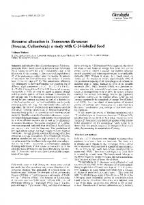
(vi) Applications could divide a large workload into small input partitions called splits, each split being a workload of a particular container. (vii) Depending on the cluster size and scheduler limitations, simultaneous containers could run in single or multiple sequential groups called waves. (viii) By default, all the containers should finish before the application submits the final output to the user. (ix) Applications may introduce different job completion time, though under the same user, input, and allocated resources. In a dynamic cloud, these parameters may change in real time. Detecting these changes is strongly dependent on the monitoring system, which should be particularly focused on the infrastructure [6]. At a generic level, we can follow a feedback-based approach based on three stages: input generation, constraint filtering, and decision-making. The general pattern is shown in Figure 1. This approach is closed. In real time, the input generation module could receive several constraints in sequence. After generating the initial parameters (by taking into account the initial constraints), an additional follow-up constraint may require another parameters calculation before being sent to the decision-making module. Consequently, the number of runs of the input generation module is proportional to the modifications (constraints) identified from the system. 2.1. Input Generation. The input generation module of AdaptCont collects or generates the required parameters for making decisions about efficient resource allocation. These parameters are as follows: (i) The input workload size. (ii) The input split size enforced by the application. (iii) The total number of available containers per each user. (iv) The wave size in which these containers may be run. (v) The constraints introduced by users. Some of these parameters are collected directly from the application. For instance, the input workload size comes in every job request. Other parameters are more complex to be generated. For instance, the number of waves 𝑤 depends on the number of input splits 𝑛𝑠 and the number of available containers per user 𝑛𝑐 , being calculated as 𝑤 = 𝑛𝑠 /𝑛𝑐 .

2.2. Constraint Filtering. This stage is needed because clouds have a limited number of costly resources. Constraints may be imposed by the infrastructure, application, and/or users. Infrastructure constraints are those constraints related to the limitation of the cloud provider, since not always the number of resources is enough for fulfilling the resource requests of all the applications and users. Some constraints are enforced by applications. For instance, some applications require a certain type of sequential container. This is the case of MapReduce systems, where, by default, containers of the first phase (map) need to finish before the containers of the second phase (reduce) start [7, 8]. Finally, other constraints are defined by users. For instance, some users have a limited capability for buying resources. 2.3. Decision-Making. Based on the parameters coming from the previous modules, the decision-making module outputs the final resource allocation. In particular, this module decides the minimum recommended container memory 𝑐RAM and CPU power 𝑐CPU per every container. This decision depends on the particular problem addressed by these containers. Once this module has decided these values for a specific application of a user, the rest of the process is automatic, since all the containers of an application are equal. This process has to be called for different applications or different users. 2.4. Predefined Containers. A possible improvement of AdaptCont is enabling the use of predefined containers with different configurations (e.g., small, medium, and large). This means that a cloud has a pool of static containers that can be used for different user request. In this way, it will not be necessary to trigger a new container, but a predefined one ready to be used. This reduces the overhead of the resource allocation process during the job submission. This feature should be part of the decision-making module. How can the framework define this pool of containers? First, it should be able to identify the typical user requests in the system. These requests may be evaluated from (i) previous (stored) monitoring values or from (ii) other monitoring variables measured at the same time, according to [9]. What happens if the container does not have the exact configuration we need? In this case, the decision-making module establishes a threshold. If the difference between the required and existing configurations is below this threshold,

4

Scientific Programming client: Client

container: Master

system: ResourceManager

container: Task

submitJob() initMaster() requestResources() allocateResources monitor() finishJob()

finish()

terminateMaster deliverResults

Figure 2: Job flow messages in Hadoop YARN: a sequence diagram.

the system uses the already existing container. Otherwise, the system triggers a new container.

3. AdaptCont Applied to YARN We have chosen as a case of study the analysis of a relevant type of a container in a specific kind of cloud systems, that is, MapReduce-based clouds. Namely, the chosen container is the application master in the next-generation MapReduce system called YARN [2]. 3.1. Background. YARN constitutes the new version of Apache Hadoop. This new implementation was built with the aim of solving some of the problems shown by the old Hadoop version. Basically, YARN is a resource management platform that, unlike the former Hadoop release, provides greater scalability and higher efficiency and enables different frameworks to efficiently share a cluster. YARN offers, among others, MapReduce capabilities. The basic idea behind YARN is the separation between the two main operations of the classic Hadoop master, resource management and job scheduling/monitoring, into separate entities or daemons. The resource manager consists of two main components: the scheduler and the application manager. While the scheduler’s duty is resource allocation, the application manager accepts job submissions and initiates the first job container for the application master. After this, the job is managed by the application master, which starts negotiating resources with the resource manager and collaborates with the node managers to run and monitor its tasks. Finally, it informs the resource manager that has been completed and releases its container. The resource manager delivers the results to the client. A simple sequence of these steps is given in Figure 2. For each job submission, the application master configuration is static and does not change for different scenarios.

According to the state-of-the-art literature [10–14], most large-scale MapReduce clusters run small jobs. As we will show in Section 4, even the smallest resource configuration of the application master exceeds the requirements of these workloads. This implies a waste of resources, which could be alleviated if the configuration is adapted to the workload size and the infrastructure resources. Moreover, some big workloads could fail if the container size is not enough for managing them. At large-scale level, this would have a higher impact. Therefore, our goal is to choose an appropriate container for the application master. 3.2. Design. In order to optimize containers for the application master, we will follow the same pattern of the general framework, that is, AdaptCont. The input generation module divides the workload input size into splits. The YARN scheduler provides containers to users, according to the number of available containers of the infrastructure each instant of time. As we mentioned above, the input generation module calculates the number of waves from the number of input splits and the number of available containers per user. Figure 3 shows how the application master manages these waves. Many constraints can be raised from the scheduler. An example of this is the phase priority. It is well known that the map phase input is by default bigger than or equal to the reduce phase input [15]. This is one of the reasons why the number of mappers is higher than the number of reducers. Due to this, as a reasonable constraint, the constraint filtering module prioritizes the number of mappers with regard to the number of reducers. Decision-making module considers mainly two parameters, total workload and wave sizes. Contrary to what it may seem at first sight, the type of application does not affect the resource allocation decision of our use case. Some applications could have more memory, CPU, or I/O

5

Application master


Container1

Container1

Container1

Container2

Container2

Container2

Container3

Container3

Container3

CPU

···

···

Containern

Containern

···

···

Memory Containern

Master Wave 1

Wave m

Wave 2 Workers

Job

Figure 3: Workers containers monitored in waves by the application master container.

requirements, influencing the number and types of needed containers. However, this would only determine the size of the worker containers, and, in this case study, our scope is focused only on the master containers, which contribute largely to the reliability of the application executions. Decision-making module uses two parameters: Ω and Ψ. The first parameter represents the minimum recommended memory size for an application master container that manages one unit wave, 𝑤unit . Our goal is to calculate 𝑐RAM from the value of Ω, with 𝑐RAM being the recommended memory size for the application master. In the same way, we aim to calculate 𝑐CPU as the recommended CPU power for the application master, from Ψ, which is the minimum recommended CPU power for an application master that manages 𝑤unit . To calculate the memory, if the actual wave 𝑤 is bigger than what could be handled by Ω, that is, bigger than 𝑤unit , then we declare a variable 𝜆 that measures this wave magnitude: 𝜆 = 𝑤/𝑤unit . Now, it is easy to find 𝑐RAM : 𝑐RAM = 𝜆 ∗ Ω + 𝑆𝑡𝑑𝑒V,

𝑆𝑡𝑑𝑒V ∈ [0;

Ω ]. 2

𝑆𝑡𝑑𝑒V ∈ [0;

Ψ ]. 2

4. Experimental Evaluation We have performed a set of experiments to validate our approach and compare it with YARN. These experiments have been made by means of simulations. In order to make this evaluation, we have followed the methodology of Section 4.1. Results of the evaluation are described in Section 4.2. Finally, the discussion about these results is shown in Section 4.3.

(1)

4.1. Methodology. To evaluate AdaptCont, we have considered three different schedulers and three different application master configurations, as is shown in Table 1. Below we give details for all of them.

(2)

Scheduler. We have taken into account three important schedulers, already implemented in YARN:

Regarding the CPU power, the formula for 𝑐CPU is 𝑐CPU = 𝜆 ∗ Ψ + 𝑆𝑡𝑑𝑒V,

daemons forms the resource manager. The resource manager has a complete knowledge about each user through the application manager and the available resources through the scheduler daemon. When the application manager receives a user request, the resource manager is informed about the workload input. The scheduler informs the application manager of every important modification regarding the monitored cluster. According to this, the application manager reacts upon the user request, by optimizing the container for its application master.

Figure 4 represents the AdaptCont modules, which are executed in the context of different YARN daemons. Whereas the input generation and the decision-making modules are part of the application manager, the constraint filtering module is part of the scheduler. The combination of both

(i) FIFO Scheduler. This was the first scheduling algorithm that was implemented for MapReduce. It works on the principle that the master has a queue of jobs, and it simply pulls the oldest job first.

6


Client

Resource manager (2) Request

Input generation

(1) Set constraints

Constraint filtering

Decision-making

(3) Authorize (4) Allocate

Scheduler

Application manager

Application master

Figure 4: AdaptCont model applied to the Hadoop YARN application master.

Table 1: Methodology description, taking into account different schedulers and masters. Scheduler FIFO Fair Capacity

YARN FIFO-YARN Fair-YARN Capacity-YARN

Master Dynamic FIFO-Dynamic Fair-Dynamic Capacity-Dynamic

Pool FIFO-Pool Fair-Pool Capacity-Pool

FIFO: FIFO scheduler. Fair: Fair scheduler. Capacity: Capacity scheduler. YARN: YARN master. Dynamic: Dynamic master. Pool: Predefined containers-based master.

(ii) Fair Scheduler. It assigns the same amount of resources (containers) to all the workloads, so that on average every job gets an equal share of containers during its lifetime. (iii) Capacity Scheduler. It gives different amount of resources (containers) to different workloads. The bigger the workload is, the more the resources are allocated to it.

(ii) Dynamic Master (Dynamic AdaptCont). This master container is adjusted in accordance with AdaptCont. Namely, it calculates the memory and CPU, according to the decision-making module and only after this does it initiate the master. (iii) Predefined Containers-Based Master (Pool AdaptCont). As defined in Section 2.4, the resource manager has a pool of master containers, which can be allocated depending on the workload size. This is an optional optimization of AdaptCont. Workload. According to the job arrival time, we consider two additional sets of experiments: (i) Set-All. In this scenario, all the jobs are already in the queue of the scheduler. We are going to combine this scenario with all the values of Table 1, since it is important to evaluate the approach under pressure, that is, when the load reaches high values.

Master. To compare YARN with AdaptCont, we use the following application master configurations:

(ii) Set-Random. This is a more realistic scenario, where jobs arrive at random times. Again, this scenario is evaluated in combination with all the values of Table 1, in order to simulate the behavior of a common MapReduce cluster.

(i) YARN Application Master (YARN). This is the default implementation of the application master in YARN.

An important parameter to take into account is the workload size. We introduce two additional scenarios:

Scientific Programming (i) Workload-Mixed. In this case, the workload size will be variable, ranging from 500 MB to 105 GB, taking (1) 500 MB, (2) 3.5 GB, (3) 7 GB, (4) 15 GB, (5) 30 GB, (6) 45 GB, (7) 60 GB, (8) 75 GB, (9) 90 GB, and (10) 105 GB as workload size inputs. We have used these boundaries, because of the average workload sizes of important production clusters. For instance, around 90% of workload inputs in Facebook [12] are below 100 GB. (ii) Workload-Same. In this case, every input (10 workloads) is the same: 10 GB. We have used this value, since, on average, the input workloads at Yahoo and Microsoft [12] are under 14 GB. Therefore, we evaluate AdaptCont with the values of Table 1 and the 4 combinations from previous scenarios: Set All-Workload Mix, Set All-Workload Same, Set RandomWorkload Mix, and Set Random-Workload Same. Constraints. In MapReduce, the application master has to manage both map and reduce workers. The map phase input is always bigger than or equal to the reduce phase input [15]. This is one of the reasons why the number of mappers is bigger than the number of reducers. On the other hand, both phases are run sequentially. Thus, we can assume as constraint that the master container resources depend on the number of mappers and not on the number of reducers. In order to simulate a realistic scenario, we have introduced in our experiments a partition failure that will impact around 10% of the cluster size. We assume that this failure appears in the fifth iteration (wave). This constraint forces AdaptCont to react in real time and adapt itself to a new execution environment, having to make decisions about future resource allocations. Setup. In our experiments, 250 containers are used for worker tasks (mappers and reducers). This number of containers is sufficient to evaluate the approach, considering 25 containers per workload. We consider that every map and reduce container is the same and can execute a particular portion (split) of the workload. Each task runs on a container that has 1024 MB RAM and 1 virtual core. According to [16–18], a physical CPU core is capable of giving optimal performance of the container, if it simultaneously processes 2 containers at most. Therefore, we take 1 CPU core as equivalent to 2 virtual cores. Our goal is to evaluate the resource utilization of the application masters, in terms of CPU and RAM. To get this, we consider an isolated set of resources oriented only to application masters. In this way, it will be easier to measure the impact of AdaptCont on saving resources. 4.2. Results. In this section, we compare the CPU and memory efficiency of YARN versus Dynamic AdaptCont and Pool AdaptCont. Before that, we analyze the wave behavior of the 10 workloads. Wave Behavior. Figure 5 represents the resource allocation (maximum number of containers or wave sizes) for the combination we have mentioned before: Set All-Workload

7 Mix, Set All-Workload Same, Set Random-Workload Mix, and Set Random-Workload Same. Figure 5(a) shows different workload sizes with the same arrival time (already in the scheduler queue). The experiments demonstrate that a maximum wave is dependent on the workload size and the scheduler. Regarding the FIFO scheduler, since the queue order is formed by the smallest workload first, for these small workloads, the maximum wave is represented by the needed containers. For instance, the first workload needs only 8 containers. This number of containers is calculated dividing the workload size by the split size (64 MB). These 8 containers are provided by the infrastructure, and this is the case of the second workload (56 containers) and the third workload (112 containers). For the fourth workload, the infrastructure is not capable of providing the needed containers, which only has 74 containers in the first wave, that is, 250 − (8 + 56 + 112). The fourth workload needs 240 containers in total. Thus, the remaining containers (240−74 = 166) will be provided in the next wave. In the second wave, since the first three workloads have finished, the scheduler will provide 166 containers to the fourth workload and the rest (250 − 166 = 84) to the fifth workload. This process is repeated until all the workloads are given the necessary containers and every job has terminated. As we can notice, the maximum wave for the latest workloads reaches higher amount of allocated containers, since the workload is bigger, and in most of the cases the scheduler is busy with a unique job. Although initially the infrastructure has 250 containers, from the fifth wave, there is a slight decrease (225), due to the partition failure (10% of the resources). This only affects the workloads not having finished before this wave (in this case, the fifth). The main drawback of the FIFO scheduler is that it may delay the completion time of the smallest jobs, especially if they arrive late to the queue. In general, this scheduler is not fair in the resource allocation and depends exclusively on the arrival time. Regarding the fair scheduler, this scheduler allocates the same number of containers to all the workloads and consequently to all the users, that is, 250/10 = 25. The partition failure forces the fair scheduler to decrease the number of containers to 22 (225/10) from the fifth wave. With regard to the capacity scheduler, this scheduler takes advantage of available resources once some jobs have finished. At the beginning, it behaves like the fair scheduler. However, when some small jobs have terminated, the available resources can be reallocated to the rest of the workloads. This is the reason why the biggest workloads in the queue get a higher number of containers. As in the previous case, the partition failure also implies a slight decrease in the number of containers from the fifth wave. Figure 5(b) represents the same mixed workloads but when they arrive randomly to the scheduler queue. Clearly, the main differences are noted in the FIFO scheduler, because the arrival time of the workloads is different and now one of the biggest workloads (9) appears in first place. The other subplots of Figure 5 show the experimental results of the same workloads with an input of 10 GB. This

Scientific Programming 300

300

250

250

200

200 Wave

Wave

8

150

150

100

100

50

50

0

1

2

3

4

5

6

7

8

9

0

10

1

2

3

4

Workload FIFO Fair

FIFO Fair

Capacity

250

250

200

200

150

100

50

50 0 2

FIFO Fair

3

4

5 6 Workload

7

8

9

10

9

10

Capacity

150

100

1

7

(b) Set Random-Workload Mix

300

Wave

Wave

(a) Set All-Workload Mix

300

0

5 6 Workload

8

9

10

Capacity (c) Set All-Workload Same

1

2

3

FIFO Fair

4

5 6 Workload

7

8

Capacity

(d) Set Random-Workload Same

Figure 5: Wave behavior: wave size according to the scheduler and the workload type.

input requires a static number of containers (in this case, 160 containers). In Figure 5(c), all the jobs have arrived to the queue. In this scenario, the FIFO allocation oscillates between the maximum wave of 160 containers and the smallest wave of 90 containers (250 − 160). This oscillation is caused by the allocation of resources to the previous workload, which does not leave enough resources for the next one, and then the cycle is repeated again. In this case, the fair and capacity schedulers have the same behavior, since all the workloads are equal. Figure 5(d) shows the number of containers for the same workload with random arrival. The difference of this scenario versus the scenario shown in Figure 5(c) is twofold: (1) The arrival of these jobs is consecutive. In every wave, a job arrives. Due to this, the FIFO scheduler is forced to wait after each round for a new workload, even though at every round there are available resources

(250 − 160 = 90), not allocated to any job. Thus, the FIFO scheduler always allocates 160 containers in every wave. (2) Whereas, in the previous scenario, the fair and capacity schedulers behave the same, in this case, the capacity scheduler acts similarly to the FIFO scheduler. This is because the capacity scheduler adapts its decisions to the number of available resources, which is enough in every moment for addressing the requirements of the jobs (160 containers). Thus, the capacity scheduler achieves a better completion time, compared to the fair scheduler. According to this analysis, we can conclude that the wave behavior and size are decisive in the application master configuration. Memory Usage. Figure 6 shows for the 4 scenarios the total memory used by the three approaches: YARN, Dynamic AdaptCont, and Pool AdaptCont.

9

12000

12000

10000

10000 Memory (MB)

Memory (MB)


8000 6000 4000

8000 6000 4000 2000

2000

0

0 FIFO

Fair

Capacity

FIFO

Scheduler YARN

Pool

YARN

Dynamic

Pool


12000

12000

10000

10000

8000

Memory (MB)

Memory (MB)

Capacity

Dynamic


6000 4000

8000 6000 4000 2000

2000 0

Fair Scheduler

FIFO

YARN

Fair Scheduler

Capacity

0

FIFO

Fair

Capacity

Scheduler Pool

Dynamic

YARN

Pool

Dynamic

(c) Set All-Workload Same


Figure 6: Memory usage and master type versus scheduler.

In the case of YARN, we have deployed the default configuration, choosing the minimum memory allocation for the application master (1024 MB). The Dynamic AdaptCont-based application master memory is dependent on the waves size. If the wave size is under 100, the decision-making module allocates a minimum recommended memory of 256 MB. For each increase of 100 in the wave size, the memory is doubled. The reasons behind this are as follows: (1) A normal Hadoop task does not need more than 200 MB [12], and this is even clearer in the case of the application master. (2) As most of the jobs are small [12–14], consequently, the maximum number of mappers is also small and, therefore, the application master requires less memory.

(3) The minimum recommended memory by Hortonworks [17] is 256 MB. The Pool AdaptCont-based application master works in a different way, constituting an alternative between the YARN master and the Dynamic master. This application master has three default configurations: small, medium, and big. The small master has 512 MB of memory, for all small jobs that need a maximum of 250 containers. The medium master has 1024 MB, as it is the default minimum YARN setting. In order to deal with big waves, the big configuration has 2048 MB. As we can see in Figure 6, YARN is outperformed by both AdaptCont approaches. YARN always consumes 10 GB, not depending on the different use cases. For instance, in Figure 6(a), Dynamic AdaptCont has memory usage of 6144 MB versus 10 GB in YARN, achieving 40% memory

10 improvement. In this case, Pool AdaptCont only uses 5120 MB, that is, 50% improvement compared to YARN. This difference between Dynamic AdaptCont and Pool AdaptCont for the FIFO scheduler is due to the way of providing memory in both approaches. If the workload needs 250 containers, Dynamic AdaptCont provides 256⌈(250/100)⌉ MB, that is, 256 ∗ 3 = 768 MB. In the same scenario, Pool AdaptCont provides 512 MB, corresponding to the small size configuration. In general, Dynamic AdaptCont is the best approach in terms of memory usage, except in the case of the FIFO scheduler, where the performance is close to and slightly worse than the performance of Pool AdaptCont. In the case of fair and capacity schedulers, Dynamic AdaptCont is the best alternative, achieving on average 75% and 67.5% improvement compared to YARN, versus 50% improvement provided by Pool AdaptCont. CPU Usage. The CPU usage is another relevant parameter to take into account. In order to measure it, we have correlated memory and CPU, considering that we need higher CPU power to process a larger amount of data, stored in memory. In YARN, you can assign a value ranging from 1 up to 32 of virtual cores for the application master. This is also the possible interval allocation for every other container. According to [16], 32 is the maximum value. In our experiments, we use the minimum value for the YARN master (1 virtual core for its container) per 1024 MB. For the Dynamic AdaptCont, the decision-making module increases the number of virtual cores after two successive increments of 256 MB of memory. This decision is based on the abovementioned methodology, which states that a physical CPU core is capable of giving optimal performance of the container, if it simultaneously processes 2 containers at most [16–18]. To be conservative, we address the smallest container, that is, a container of 256 MB. For instance, if the memory usage is 768 MB, the chosen number of virtual cores is 2. The same strategy is valid for the Pool AdaptCont, assuming 1 virtual core for small containers, 2 virtual cores for medium containers, and 3 virtual cores for large containers. Due to this policy, the CPU does not change so abruptly as the memory for Dynamic and Pool AdaptCont. Thus, as is shown in Figure 7, both approaches behave similarly, except in the case of FIFO with Workload Mix. This was previously justified in the memory usage evaluation. As the CPU is proportional to the memory usage, the behavior of Dynamic AdaptCont with FIFO for Workload Mix is again repeated in the case of CPU. In most of the cases, the improvement of both Dynamic and Pool AdaptCont against YARN reaches 50%. 4.3. Discussion. In this section, we discuss what combination of approaches and schedulers can be beneficial in common scenarios. As a result of the experiments, we can conclude that YARN used by default is not appropriate for optimizing the use of MapReduce-based clouds, due to the waste of resources.

Scientific Programming In the presence of heavy and known advanced workloads (this is the usual case of scientific workloads), according to our results, the best recommended strategy is to use Dynamic AdaptCont combined with FIFO scheduler. However, if we have limited resources per user, a better choice could be Dynamic AdaptCont combined with fair scheduler. This scheduler allocates a small set of resources to every workload, improving the overall performance. In a scenario where we have a mixture of large and small workloads, the choice should be Dynamic AdaptCont combined with capacity scheduler. This is due to the adaptability of this scheduler with regard to the input workload and available resources. Finally, as shown in the experiments, if our focus is on CPU and not on memory, we can decide to use Pool AdaptCont (combined with any schedulers) instead of the dynamic approach.

5. Related Work As far as we know, this paper is the first contribution that proposes a MapReduce optimization through container management. In particular, linked to our use case, it is the first contribution that aims to create reliable masters, by means of the allocation of sufficient resources to their containers. There are many contributions on MapReduce whose goal is optimizing the framework from different viewpoints. An automatic optimization of the MapReduce programs has been proposed in [19]. In this work, authors provide out-of-the-box performance for MapReduce programs that need to be run using as input large datasets. In [20], an optimization system called Manimal was introduced, which analyzes MapReduce programs by applying appropriate dataaware optimizations. The benefit of this best-effort system is that it speeds up these programs in an autonomic way, without human intervention. In [21], a new classifications algorithm is introduced with the aim of improving the data locality of mappers and the task execution time. All these contributions differ from our contribution since they are only software-oriented optimizations for the MapReduce pipeline, and they do not take into account the resource allocation or the CPU and memory efficiency. FlexSlot [22] is an approach that resizes map slots and changes the number of slots of Hadoop in order to accelerate the job execution. With the same aim, DynamicMR [23] tries to relax the slot allocation constraint between mappers and reducers. Unlike our approach, FlexSlot is only focused on the map stage and both FlexSlot and DynamicMR do not consider the containers as resource allocation facility. In [24], authors introduce MRONLINE, which is able to configure relevant parameters of MapReduce online, by collecting previous statistics and predicting the task configuration in fine-grain level. Unlike MRONLINE, AdaptCont uses a feedback-control approach that also enables its application to single points of failure. Cura [25] automatically creates an optimal cluster configuration for MapReduce jobs, by means of the framework profiling, reaching global resource optimization. In addition, Cura introduces a secure instant VM allocation to reduce

11

12

12

10

10

8

8

CPU (core)

CPU (core)


6 4

4 2

2 0

6

FIFO

Fair

0

Capacity

FIFO

Scheduler Pool

YARN

Dynamic



12

12

10

10

8

8 CPU (core)

CPU (core)

Capacity

Pool

YARN

Dynamic

6 4 2 0

Fair Scheduler

6 4 2

FIFO

Fair Scheduler

Capacity

Pool

YARN Dynamic

0

FIFO

Capacity

Fair Scheduler

YARN

Pool

Dynamic

(c) Set All-Workload Same


Figure 7: CPU usage and master type versus scheduler.

the response time for the short jobs. Finally, it applies other resource management techniques such as cost-aware resource provisioning, VM-aware scheduling, and online VM reconfiguration. Overall, these techniques lead to the enhancement of the response time and reduce the resource cost. This proposal differs from our work, because it is mostly concentrated in particular workloads excluding others. Furthermore, it is focused on VMs management and not on containers, as AdaptCont. Other proposals aim to improve the reliability of the MapReduce framework, depending on the executional environment. The work proposed in [26] is a wider review that includes byzantine failures in Hadoop. The main properties upon which the UpRight library is based are safety and eventual liveliness. The contribution of this paper is to establish byzantine fault tolerance as a viable alternative to crash fault tolerance for at least some cluster services rather than any individual technique.

The work presented in [27] represents a byzantine faulttolerant (BFT) MapReduce runtime system that tolerates faults that corrupt the results of computation of tasks, such as the cases of DRAM and CPU errors/faults. The BFT MapReduce follows the approach of executing each task more than once, but in particular circumstances. This implementation uses several mechanisms to minimize both the number of copies of tasks executed and the time needed to execute them. This approach has been adapted to multicloud environments in [28]. In [29], authors propose another solution for intentional failures called Accountable MapReduce. This proposal forces each machine in the cluster to be responsible for its behavior, by means of setting a group of auditors that perform an accountability test that checks the live nodes. This is done in real time, with the aim of detecting the malicious nodes. In order to improve master reliability, [30] proposes to use a clone master. All the worker nodes should report their

12


activity to this clone master. For unstable environments, some other works [31–33] introduce dedicated nodes for the main daemons, including the master daemon. Unlike our approach, these contributions related to reliability do not deal with the resource utilization.

[3]

6. Conclusions

[4]

The classic Apache Hadoop (MapReduce 1.0) has evolved for a long time by means of the release of several versions. However, the scalability limitations of Hadoop have only been solved partially with Hadoop YARN (MapReduce 2.0). Nevertheless, YARN does not provide an optimum solution to resource allocation, specifically at container level, causing both performance degradation and unreliable scenarios. This paper proposes AdaptCont, a novel optimization framework for resource allocation at the container level, based on feedback systems. This approach can use two different selection algorithms, Dynamic AdaptCont and Pool AdaptCont. On the one hand, Dynamic AdaptCont figures out the exact amount of resources per each container. On the other hand, Pool AdaptCont chooses a predefined container from a pool of available configurations. The experimental evaluation demonstrates that AdaptCont outperforms the default resource allocation mechanism of YARN in terms of RAM and CPU usage, by a range of improvement from 40% to 75% for memory usage and from 15% to 50% for CPU utilization. As far as we know, this is the first approach to improve the resource utilization at container level in MapReduce systems. In particular, we have optimized the performance of the YARN application master. As future work, we will explore the adaptation of AdaptCont for other containers of MapReduce worker tasks and deploy AdaptCont on real distributed infrastructures. We also expect to explore AdaptCont for VMs, in particular for allocating raw VMs to different user requests. We believe that fine-tuning a VM can be optimized, driven by requirements coming from an intersection between performance, reliability, and energy efficiency.

[5]

[6]

[7]

[8]

[9]

[10]

[11]

[12]

[13]

Competing Interests The authors declare that they have no competing interests. [14]

Acknowledgments The research leading to these results has received funding from the H2020 project Reference no. 642963 in the call H2020-MSCA-ITN-2014.

[15] [16]

References [17] [1] J. Dean, S. Ghemawat, and Google Inc, “MapReduce: simplified data processing on large clusters,” in Proceedings of the 6th Conference on Symposium on Operating Systems Design & Implementation (OSDI ’04), USENIX Association, San Francisco, Calif, USA, December 2004. [2] V. K. Vavilapalli, A. C. Murthy, C. Douglas et al., “Apache hadoop YARN: yet another resource negotiator,” in Proceedings

[18]

of the 4th Annual Symposium on Cloud Computing (SoCC ’13), pp. 5:1–5:16, ACM, Santa Clara, Calif, USA, 2013. N. R. Herbst, S. Kounev, and R. Reussner, “Elasticity in cloud computing: what it is, and what it is not,” in Proceedings of the 10th International Conference on Autonomic Computing (ICAC ’13), pp. 23–27, USENIX, San Jose, Calif, USA, 2013. K. J. Astrom and R. M. Murray, Feedback Systems: An Introduction for Scientists and Engineers, Princeton University Press, Princeton, NJ, USA, 2008. M. Armbrust, A. Fox, R. Griffith et al., “Above the clouds: a berkeley view of cloud computing,” Tech. Rep., University of California, Berkeley, Calif, USA, 2009. J. Montes, A. Sánchez, B. Memishi, M. S. Pérez, and G. Antoniu, “GMonE: a complete approach to cloud monitoring,” Future Generation Computer Systems, vol. 29, no. 8, pp. 2026–2040, 2013. A. Verma, B. Cho, N. Zea, I. Gupta, and R. H. Campbell, “Breaking the MapReduce stage barrier,” Cluster Computing, vol. 16, no. 1, pp. 191–206, 2013. T.-C. Huang, K.-C. Chu, W.-T. Lee, and Y.-S. Ho, “Adaptive combiner for MapReduce on cloud computing,” Cluster Computing, vol. 17, no. 4, pp. 1231–1252, 2014. F. Salfner, M. Lenk, and M. Malek, “A survey of online failure prediction methods,” ACM Computing Surveys, vol. 42, no. 3, article 10, 2010. S. Y. Ko, I. Hoque, B. Cho, and I. Gupta, “Making cloud intermediate data fault-tolerant,” in Proceedings of the 1st ACM Symposium on Cloud Computing (SoCC ’10), pp. 181–192, ACM, New York, NY, USA, June 2010. F. Dinu and T. S. Eugene Ng, “Understanding the effects and implications of compute node related failures in Hadoop,” in Proceedings of the 21st ACM Symposium on High-Performance Parallel and Distributed Computing (HPDC ’12), pp. 187–197, Delft, The Netherlands, June 2012. R. Appuswamy, C. Gkantsidis, D. Narayanan, O. Hodson, and A. Rowstron, “Scale-up vs scale-out for hadoop: time to rethink?” in Proceedings of the 4th Annual Symposium on Cloud Computing (SOCC ’13), pp. 20.1–20.13, ACM, New York, NY, USA, 2013. G. Ananthanarayanan, A. Ghodsi, A. Wang et al., “PACMan: coordinated memory caching for parallel jobs,” in Proceedings of the 9th USENIX Conference on Networked Systems Design and Implementation (NSDI ’12), p. 20, USENIX Association, Berkeley, Calif, USA, 2012. K. Elmeleegy, “Piranha: optimizing short jobs in hadoop,” Proceedings of the VLDB Endowment, vol. 6, no. 11, pp. 985–996, August 2013. T. White, Hadoop: The Definitive Guide: Storage and Analysis at Internet Scale, O’Reilly, 3rd edition, 2012. Apache Software Foundation, Apache Hadoop NextGen MapReduce (YARN), 2015, http://hadoop.apache.org/docs/current/ hadoop-yarn/hadoop-yarn-site/YARN.html. Hortonworks, Hortonworks Data Platform: Installing HDP Manually, 2013. M. Zaharia, D. Borthakur, J. Sen Sarma, K. Elmeleegy, S. Shenker, and I. Stoica, “Delay scheduling: a simple technique for achieving locality and fairness in cluster scheduling,” in Proceedings of the 5th ACM EuroSys Conference on Computer Systems (EuroSys ’10), pp. 265–278, ACM, Paris, France, April 2010.

Scientific Programming [19] S. Babu, “Towards automatic optimization of MapReduce programs,” in Proceedings of the Proceedings of the 1st ACM Symposium on Cloud Computing, pp. 137–142, ACM, New York, NY, USA, June 2010. [20] E. Jahani, M. J. Cafarella, and C. Ré, “Automatic optimization for MapReduce programs,” Proceedings of the VLDB Endowment, vol. 4, no. 6, pp. 385–396, 2011. [21] Z. Tang, J. Zhou, K. Li, and R. Li, “A MapReduce task scheduling algorithm for deadline constraints,” Cluster Computing, vol. 16, no. 4, pp. 651–662, 2013. [22] Y. Guo, J. Rao, C. Jiang, and X. Zhou, “FlexSlot: moving hadoop into the cloud with flexible slot management,” in Proceedings of the International Conference for High Performance Computing, Networking, Storage and Analysis (SC ’14), pp. 959–969, IEEE Press, New Orleans, La, USA, November 2014. [23] S. Tang, B.-S. Lee, and B. He, “DynamicMR: a dynamic slot allocation optimization framework for mapreduce clusters,” IEEE Transactions on Cloud Computing, vol. 2, no. 3, pp. 333– 347, 2014. [24] M. Li, L. Zeng, S. Meng et al., “MRONLINE: mapReduce online performance tuning,” in Proceedings of the ACM 23rd International Symposium on High-Performance Parallel and Distributed Computing (HPDC ’14), pp. 165–176, New York, NY, USA, 2014. [25] B. Palanisamy, A. Singh, L. Liu, and B. Langston, “Cura: a costoptimized model for MapReduce in a cloud,” in Proceedings of the 27th IEEE International Parallel and Distributed Processing Symposium (IPDPS ’13), pp. 1275–1286, IEEE, Boston, Mass, USA, May 2013. [26] A. Clement, M. Kapritsos, M. Kapritsos et al., “Upright cluster services,” in Proceedings of the ACM SIGOPS 22nd Symposium on Operating Systems Principles (SOSP ’09), pp. 277–290, New York, NY, USA, 2009. [27] P. Costa, M. Pasin, A. Bessani, and M. Correia, “Byzantine faulttolerant MapReduce: faults are not just crashes,” in Proceedings of the 3rd IEEE International Conference on Cloud Computing Technology and Science (CLOUDCOM ’11), pp. 17–24, IEEE Computer Society, Washington, DC, USA, 2011. [28] M. Correia, P. Costa, M. Pasin, A. Bessani, F. Ramos, and P. Verissimo, “On the feasibility of byzantine fault-tolerant mapreduce in clouds-of-clouds,” in Proceedings of the 31st Symposium on Reliable Distributed Systems (SRDS ’12), pp. 448–453, IEEE, Irvine, Calif, USA, October 2012. [29] Z. Xiao and Y. Xiao, “Achieving accountable MapReduce in cloud computing,” Future Generation Computer Systems, vol. 30, no. 1, pp. 1–13, 2014. [30] F. Wang, J. Qiu, J. Yang, B. Dong, X. Li, and Y. Li, “Hadoop high availability through metadata replication,” in Proceedings of the 1st International Workshop on Cloud Data Management (CloudDB ’09), pp. 37–44, ACM, Hong Kong, November 2009. [31] H. Lin, X. Ma, and W.-C. Feng, “Reliable MapReduce computing on opportunistic resources,” Cluster Computing, vol. 15, no. 2, pp. 145–161, 2012. [32] N. Chohan, C. Castillo, M. Spreitzer, M. Steinder, A. Tantawi, and C. Krintz, “See Spot Run: using spot instances for mapreduce workflows,” in Proceedings of the 2nd USENIX Conference on Hot Topics in Cloud Computing (HotCloud ’10), p. 7, USENIX Association, Berkeley, Calif, USA, 2010. [33] H. Liu, “Cutting mapReduce cost with spot market,” in Proceedings of the 3rd USENIX Conference on Hot Topics in Cloud Computing (HotCloud ’11), p. 5, Berkeley, Calif, USA, 2011.

13

Journal of

Advances in

Industrial Engineering

Multimedia

Hindawi Publishing Corporation http://www.hindawi.com

The Scientific World Journal Volume 2014


Volume 2014

Applied Computational Intelligence and Soft Computing

International Journal of

Distributed Sensor Networks Hindawi Publishing Corporation http://www.hindawi.com

Volume 2014


Volume 2014


Volume 2014

Advances in

Fuzzy Systems Modelling & Simulation in Engineering Hindawi Publishing Corporation http://www.hindawi.com


Volume 2014

Volume 2014

Submit your manuscripts at http://www.hindawi.com

Journal of

Computer Networks and Communications

Advances in

Artificial Intelligence Hindawi Publishing Corporation http://www.hindawi.com


Volume 2014


Biomedical Imaging

Volume 2014

Advances in

Artificial Neural Systems


Computer Engineering

Computer Games Technology



Advances in

Volume 2014

Advances in

Software Engineering Volume 2014


Volume 2014


Volume 2014


Volume 2014


Reconfigurable Computing

Robotics Hindawi Publishing Corporation http://www.hindawi.com

Computational Intelligence and Neuroscience

Advances in

Human-Computer Interaction

Journal of

Volume 2014


Volume 2014


Journal of

Electrical and Computer Engineering Volume 2014


Volume 2014


Volume 2014