Jan 14, 2015 - Printed 16 January 2015. (MN LATEX style file v2.2) ... objects of our sample. The knowledge of the black hole mass and disc luminosity helps to.
Mon. Not. R. Astron. Soc. 000, 1–?? (2012)
Printed 16 January 2015
(MN LATEX style file v2.2)
Fermi/LAT broad emission line blazars G. Ghisellini ⋆, F. Tavecchio INAF – Osservatorio Astronomico di Brera, via E. Bianchi 46, I–23807 Merate, Italy
16 January 2015
arXiv:1501.03504v1 [astro-ph.HE] 14 Jan 2015
ABSTRACT
We study the broad emission line blazars detected in the γ–ray band by the Large Area Telescope onboard the Fermi satellite and with the optical spectrum studied by Shaw et al. (2012, 2013). The observed broad line strength provides a measure of the ionizing luminosity of the accretion disk, while the γ–luminosity is a proxy for the bolometric non–thermal beamed jet emission. The resulting sample, composed by 217 blazars, is the best suited to study the connection between accretion and jet properties. We compare the broad emission line properties of these blazars with those of radio–quiet and radio–loud quasars present in the Sloan Digital Sky Survey, to asses differences and similarities of the disc luminosity and the virial black hole mass. For most sources, we could derive the black hole mass by reproducing the IR–optical–UV data with a standard accretion disc spectrum, and we compared the black hole masses derived with the two methods. The distributions of the masses estimated in the two ways agree satisfactorily. We then apply a simple, one–zone, leptonic model to all the 217 objects of our sample. The knowledge of the black hole mass and disc luminosity helps to constrain the jet parameters. On average they are similar to what found by previous studies of smaller samples of sources. Key words: galaxies: BL Lacertae objects: general — galaxies: quasars: general — radiation mechanisms: non-thermal —
1 INTRODUCTION Blazars are extragalactic radio–loud sources whose jet is pointing toward us (for recent reviews, see e.g. B¨ottcher 2007; Ghisellini 2011; Dermer 2014). To be more precise, we may define blazars as the sources whose jet axis is at an angle sin θv 6 1/Γ with respect to the line of sight, where Γ is the bulk Lorentz factor. This implies that for each observed blazars, there are other 2Γ2 intrinsically identical sources, but pointing in other directions. Blazars are classically divided in two subclasses: Flat Spectrum Radio Quasars (FSRQs) and BL Lacs. The usual divide between the two subclasses is based on the Equivalent width (EW) of the optical ˚ (rest frame, Urry & broad emission lines: BL Lacs have EW10) FSRQ (S12) total FSRQ (S12) studied in this paper BL Lacs (S13) total BL Lacs (S13) with z BL Lacs (S13) studied in this paper Total blazars studied in this paper
105,783 89,783 9,393 8,257 229 191 475 209 26 217
Table 1. Number of sources in the different samples. Note that the objects studied by S12 and S13 are all detected in γ–rays by Fermi/LAT.
2.2 BL Lacs in Shaw et al. (2013) Shaw et al. (2013, hereafter S13) studied a very large sample of BL Lac objects present on the second Fermi catalog of AGN (2LAC, Ackermann et al. 2011). In the original 2LAC sample, there are 410 BL Lacs, 357 FSRQs and 28 AGN of other known types, and 326 AGN of unknown type. S13 themselves were able to classify some of the several “unknown type” AGNs present in the 2LAC catalog, increasing the number of BL Lacs to 475, and decreasing the number of the sources of unknown type to 215. By spectroscopically observing a large number of BL Lacs, and by adding BL Lacs of already known redshift, they assembled a sample of 209 BL Lac with the redshift spectroscopically measured. In addition, they could constrain the redshift of other 241 BL Lacs (finding a lower limit on the redshift, see S13 for details and their Tab. 1 for a break down on the number of known redshift for source type). By visually inspecting all SED of the BL Lacs with redshifts, we selected the 26 objects with a clear presence of broad emission lines. Although they are classified as BL Lacs according to the classical definition (rest frame equivalent width of the emission line less than ˚ they should be rather considered to belong to the tail, at low 5 A), accretion luminosities, of FSRQs, and for this reason we include them in our sample.
2 THE SAMPLES We selected our sources from the FSRQs of Shaw et al. (2012) and the BL Lacs of Shaw et al. (2013). We compare them with the radio–quiet and radio–loud quasars of Shen et al. (2011). Tab. 1 shows a break down of the samples.
2.1 FSRQs in Shaw et al. (2012) All our Fermi/LAT FSRQs come from the sample of Shaw et al. (2012, hereafter S12). The sample includes 229 objects, present in the 1LAC sample of Abdo et al. (2010), that have been spectroscopically observed by Shen et al. (2012; 165 sources) or by the SDSS Data Release 7 (DR7, Shen et al. 2011, 64 objects). Of these, we have studied the 191 objects with enough multiwavelength information necessary to apply our model. The S12 sample of FSRQs does not include several bright and famous blazars with historical spectroscopic classifications in the literature.
2.3 Quasars in Shen et al. (2011) Shen et al. (2011, heafter S11) studied a large number of quasars selected from the SDSS (Schneider et al. 2010) according to the following criteria: i) the (rest frame) FWHM of the broad lines greater than 1,000 km s−1 , and ii) the absolute magnitude is brighter than Mi =–22.0 The quasars selected in this way are 105,783. We then selected the region of the sky covered by the FIRST survey. In this region there are 89,783 quasars that have been observed, but not detected by the FIRST (with 1 mJy flux limit at 1.4 GHz). For brevity, we call these sources “radio–quiet”. Moreover, there are 9,393 radio–detected quasars. Of these, there are 8,257 radio–loud sources, i.e. objects with a radio–loudness RL > 10. The radio– loudness is defined as in S11, i.e. the ratio of the rest frame 5 ˚ flux, where the 5 GHz flux is extrapoGHz flux and the 2500 A lated from the observed 1.4 GHz flux (assuming a power law slope Fν ∝ ν −0.5 ). c 2012 RAS, MNRAS 000, 1–??
Fermi/LAT broad emission line blazars
Figure 1. Redshift distribution of the FSRQs in our sample (red hatched), compared with radio–loud sources (RL > 10, black) and radio–quiet (green) quasars of S11. The distributions are “normalized” (i.e. the number of the sources at the peak of the distribution has been set equal to one). The blue hatched distribution is for the 26 BL Lacs in our sample. γ–loud FSRQs have a slightly smaller redshift of both radio–loud and radio–quiet quasars, that share a similar redshift distribution.
3 GENERAL OBSERVED PROPERTIES 3.1 Redshift distribution In Fig. 1 the redshift distribution of the FSRQs in our sample is compared to those of radio–loud sources (radio–loudness R > 10) and radio–quiet quasars. These distribution are normalized (namely, the number of the sources at the peak of the distribution has been set to one). We also show the redshift distribution for the 26 BL Lacs in our sample. It can be seen that the Fermi/LAT blazars have, on average, smaller redshifts. This is likely due to the still high sensitivity threshold of the γ–ray flux: to enter the γ–ray catalog, the typical blazar must be closer than a critical redshift.
3.2 Broad line luminosity distributions The three more prominent broad emission lines considered by S12 in FSRQs are Hβ, MgII and CIV. S12 provide the Full Width Half Maximum (FWHM) and the luminosity of these lines. According to the redshift range, one can find in the optical spectrum only one or two of these lines, but never all three together. The method of line fitting is very similar to the one used by S11 for analyzing his sample of quasars (both radio–loud and radio–quiet). The comparison between the line luminosity distributions of the S12 γ–ray blazars and the entire S11 population of quasars is shown in S12 (their Fig. 2). We show in Fig. 2 how the line luminosity distributions of γ– loud blazars compare with radio–loud and radio–quiet quasars. One can see that the Hβ luminosity distributions are very similar, while the MgII and especially the CIV luminosities for γ–loud blazars tend to be slightly under–luminous. The line luminosity distribution of radio–loud and radio–quiet are instead always similar. This c 2012 RAS, MNRAS 000, 1–??
3
Figure 2. Distribution of the luminosities of the three most prominent broad emission lines of the blazars in our sample (red hatched), compared with radio–loud blazars (radio–loudness RL > 10, black) and radio–quiet (green) quasars of the S11 sample. The distributions are almost the same. Note that the trend of increasing luminosity (from the Hβ to the CIV luminosity distribution) is an effect of the increasing average redshift.
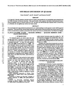
reflects the different redshift distribution of the blazars in our sample, that extends to lower values than the quasars in the S11 sample (see Fig. 1). An estimate of the black hole mass based on the virial method exists for all FSRQs in our sample (see §3.3). All values are reported in Tab. 3, together with the black hole mass we have derived by fitting the optical–UV continuum with a disc spectrum (see §3.3). Both S11 and S12 use the same virial method. In Fig. 3 we compare the line luminosities as a function of the virial mass. When more than one broad emission line is used to derive more than one value of the black hole mass, we took the logarithmic average of the different values. Green (black) dots are the radio–quiet (radio–loud) quasars, red circles are the γ–loud blazars. The γ–loud blazars tend to have smaller (virial) black hole masses than the rest of the sources. This effect was noted also by S12, that suggested a possible selection effect: blazars are highly aligned sources, and if the broad line region is not spherically symmetric, but flattened toward the disk (see e.g. Shen & Ho 2014), we should observe lines systematically narrower than observed in misaligned objects (Decarli et al. 2011), leading to a smaller estimate of the black hole mass (see §3.3).
3.3 Black hole mass Virial mass — The virial method to estimate the black hole mass is now the most widely used, allowing to measure the black hole mass of hundred thousand objects in a automatic or semi–automatic way. However, the measurement, besides being based on the virial assumption (the motion of the broad line clouds is governed by gravity) is not direct, but is necessarily based on correlations with
4
G. Ghisellini & Tavecchio
Figure 3. Luminosities of the three main broad emission lines as a function of the black hole mass estimated by S11 for the radio–quiet (green) and radio–loud (black) AGN, and by S12 for the γ–ray blazars (red circles). Both studies base the black hole mass estimate on virial arguments, using the FWHM of the lines and the radius of the BLR estimated through the radius–ionizing luminosity correlation.
their own dispersions that are not simply due to measurement errors. The uncertainty associated to these estimates is large, of the order of 0.5–0.6 dex. Vestergard et al. (2006) and Park et al. (2012) estimated that the black hole mass derived in this way has an uncertainty of a factor ∼3–4. Besides this, there are two additional concerns: i) the geometry of the broad line region can influence the observed FWHM of the lines. Decarli et al. (2008) pointed out that a flattened BLR (i.e. not spherical, but with clouds distributed closer to the accretion disc) observed close to the normal of the accretion disc shows lines of narrower FWHM. ii) Marconi et al. (2008) noted that if the accretion disc is emitting close to the Eddington rates, one should account for the radiation pressure force exerted on the broad line clouds: to be balanced, one needs more gravity, hence a bigger black hole mass. Tab. 3 (in the Appendix) reports the black hole masses derived by Shaw et al. (2012) through the virial method. Disc–fitting mass — The spectrum of the emission produced by a standard, Shakura & Sunyaev (1973) disc is a superposition of black–body spectra with temperature distribution T (R), where R is the distance form the black hole, depending only on the black hole mass M and the accretion rate M˙ . Assuming an efficiency η defined by Ld = η M˙ c2 , where Ld is the bolometric disc luminosity, the observations allow us to directly fix M˙ , in two possible ways (see also Calderone et al. 2013; Castignani et al. 2013). We could in fact directly observe the optical–UV hump produced by the disc, corresponding to its maximum. The peak of the νLν disc spectrum is ∼ Ld /2. We can then infer M˙ directly, once a value for the efficiency η is assumed (we here assume η= 0.08). If the peak of the disc emission is not well sampled, because it lies outside the observable range or because it is “contaminated” by
Figure 4. Two examples for deriving the black hole mass. In the top panel ˙ can be derived directly, even withthe disc emission is well defined, and M out the knowledge of the broad line luminosities (that should in any case give consistent results). Changing the black hole mass implies different peak frequencies, but same peak luminosity (grey stripe). The black hole mass is the one best accounting for the optical–UV data. The bottom panel shows that the jet emission can sometimes dominate the optical–UV band, hiding the disc emission (and the observed optical spectrum, taken at a different time). In this case the disc luminosity is found through the luminosity of the broad emission lines. The black hole mass is found requiring that the jet+disc luminosity matches the optical–UV data, especially in the low state.
the jet emission or by the host galaxy, we can infer Ld through the luminosity of the broad emission lines. According to the template of Francis et al. (1991), setting the relative weight of the Lyα luminosity equal to 100, we have that the weight of the luminosity of all broad lines is 556, with the broad hydrogen Hα, Hβ, MgII and CIV contributing 77, 22, 34 and 63, respectively (see also Celotti, Padovani & Ghisellini 1997; vanden Berk et al. 2001). If more of one line is present, we take the logarithmic average of the broad line region luminosity LBLR derived by the single lines. We then assume that LBLR is a fixed fraction – 10% – of Ld . This fixes M˙ . For a given M˙ (i.e. for a given Ld ), the black hole mass regulates the peak frequency of the disk emission (heavier black holes have larger Schwarzschild radii, and thus colder discs). In other words, the knowledge of Ld fixes the peak value of the νLν emission of the disc, but a change of the black hole mass corresponds to an horizontal shift in a νLν plot. Therefore, in principle, even one data point is enough to fix the black hole mass, if we are sure that it belong to the disc emission. This of course is often questionable. In some (16) cases, there is only one optical point to constrain the black hole mass, with no indications of an upturn of the SED, characteristic of the presence of the accretion disc emission. These blazars are marked with an asterisk in the last column of Tab. 3. These are the values used for the jet model (see below). The uncertainty on the resulting black hole mass therefore depends on the quality of the data. If the maximum of the disc spectrum is visible, the uncertainties are less than a factor 2, better than the virial method. Fig. 4 illustrates two examples of how we derive the black hole mass through the disc fitting method. In the first case (top panel) the disc contribution is well defined, and its lumic 2012 RAS, MNRAS 000, 1–??
Fermi/LAT broad emission line blazars
Figure 5. Black hole mass estimated through the disk fitting method (in this paper) as a function of the black hole mass estimated with the virial method by S12, for all the FSRQs studied in this paper. Only blazars with independent disc–fitting values are included (i.e. we have excluded all blazars with values of the disc–fitting mass indicated between parentheses in Tab. 3, and all BL Lacs). Different symbols correspond to the different lines used for the virial mass. The diagonal line is the equality line. The grey stripe indicates a factor 4 uncertainty on the virial mass.
nosity can be inferred directly. Sometimes it can disagree with Ld derived from the broad line luminosity. In this case we prefer the value directly observed. On the contrary, when the disc emission is diluted by the jet flux (as in the bottom panel of Fig. 4), we set Ld = 10LBLR . We then find M by fitting the disc+jet emission to the data. As long as there is some sign of emission disc flux (typically, an upturn at high optical–UV frequencies) the estimate is reliable. Less so when there is no sign of disc emission. A broad < < limiting range is set by requiring that 10−2 LEdd ∼ Ld ∼ LEdd : the lower limit is given by requiring that the accretion disc is radiatively efficient, and so it can photo–ionize the BLR, while the upper limit requires the source to be sub–Eddington. Within the corresponding range of masses, the accretion disk cannot overproduce any existing data, and often this requirement narrows down the black hole mass range. We admittedly use a rough simplification for the disc model, by using a Shakura & Sunyaev (1973) disc. In reality, it is likely that the black hole is spinning, perhaps rapidly, and this implies a greater overall efficiency, since the last stable orbit moves inwards by increasing the black hole spin. On the other hand the spectrum produced by a disc surrounding a Kerr hole is different from the one of a Shakura–Sunyaev disk only at the highest frequencies (innermost orbits), where it emits a greater luminosity. Consider a standard Shakura–Sunyaev disc and a disc around a Kerr hole emitting the same Ld . The spectrum of the disc around the Kerr hole would peak at higher UV frequencies, and therefore it will be dimmer at IR frequencies. To match those with the data, we will be obliged to increase the black hole mass (i.e. to assume a large surface, hence a smaller temperature). We thus conclude that it is possible that the mass derived here are slightly underestimated, but by an amount which is smaller than the overall uncertainties (which are around a factor 2–3). c 2012 RAS, MNRAS 000, 1–??
5
Figure 6. Distribution of the black hole masses of γ–ray loud blazars estimated through disk fitting (red hatched) and through the virial method (blue hatched). We have excluded all blazars whose disc–fitting black hole mass is given between parentheses in Tab. 3, and all BL Lacs. The masses estimated by the two methods, on average, differ only slightly (less than ∼ 0.2 dex). Both distributions are fitted with a log–normal function, whose width is indicated.
Bearing in mind this caveat, we could apply the disc–fitting method to 116 FSRQs, while for the remaining 75 FSRQs the data were too poor, or the synchrotron jet component too dominant. Tab. 3 reports the value of the derived black hole mass. The values in parenthesis could not be evaluated through the disc–fitting method. In most cases these values have been set equal to the virial masses (within a factor ∼2–3, denoted by “–” in the last column). In a minority of cases they differ from the virial values for the following reasons, as flagged in the last column: 1) a value larger than the virial one has been adopted to avoid super Eddington or nearly Eddington disc luminosities; 2) a value smaller than the virial one has been adopted to avoid to overproduce the NIR–optical flux; 3) a value larger than the virial one has been adopted to avoid to overproduce the optical–UV flux. In the following we will consider, as black hole masses derived through the disc–fitting method, only the 116 values for which we could independently derived the mass with this method. Also, we do not consider the values derived for BL Lacs. In Fig. 5 we compare the black hole mass derived through the disc fitting method with the virial masses of the same objects. There is a general agreement, with a large dispersion. The horizontal width of the grey stripe indicates a factor 4 uncertainty for the virial masses. The virial masses are shown with different symbols according to the line used, but there seems to be no systematic trend. Fig. 6 compares the distributions of the 116 values of the black hole masses derived by the two methods. Fitting the (logarithmic) distributions with a log–normal, we derived σ = 0.4 for the blazar masses derived with disc fitting, and σ = 0.5 for the virial masses. Also the average values differ, but slightly (less than ∼0.2 dex).
6
G. Ghisellini & Tavecchio the reader to that paper for a full discussion of the features of the model, we here emphasize that the knowledge of the black hole mass and of the luminosity of the accretion disc considerably helps to constrain the free parameters of the model itself. In the following we summarize the model parameters and the observables that we can use to fix them. 4.1 Parameters of the model
Figure 7. Normalized distribution of the disk luminosity on Eddington units for our blazars (red), radio–loud (black line) and radio–quiet (green) AGN in S11. For all sources the disc luminosity and the black hole mass are estimated through the line luminosity and the mass through the virial method (see Fig. 5 for a comparison of the two estimates for the γ–ray loud blazars). The blue hatched distribution is for the BL Lac objects studied in this paper.
3.4 Disc luminosity Fig. 7 shows the distribution of disc luminosities measured in Eddington units for our blazars (normalized at the peak, set equal to one), compared with radio–loud and radio–quiet quasars of S11. The accretion disc luminosity Ld and the black hole mass M of all objects, including the γ–ray loud blazars, have been found through the broad line luminosities and the virial method, respectively. The blazar distribution peaks at Ld /LEdd ∼ 0.1, with a small dispersion. Fitting this distribution with a log–normal function we derive σ = 0.3, with a tail towards small values made by BL Lac objects. The distributions of the S11 radio–quiet and radio–loud objects peak at a value slightly less than one tenth Eddington and their dispersions are both broader than the one of blazars. This is likely due to the fact that hLd /LEdd i for all distributions is similar, but that radio–loud sources with discs accreting below some value < (Ld ∼ 0.1–0.03 LEdd ) go undetected in the γ–ray band, even with the sensitivity of Fermi/LAT. Usually, we set Ld equal to the value derived through the broad emission lines. There are a few cases when this value conflicts with existing data, as made evident by the accretion disc spectrum we construct. In these cases we have changed Ld , taking the value derived through disc fitting. Roughly 10% of the sources have values of Ld calculated through the broad lines and through disc– fitting that disagree by a factor between 2 and 5. This can be explained, since when we calculate Ld through the broad lines we use a template that has a factor 2 (1σ) uncertainty (Calderone et al. 2013). Therefore, statistically, ∼10% of outliers are expected.
4 THE JET MODEL To interpret the overall SED of our blazars, we use the one–zone leptonic model of Ghisellini & Tavecchio (2009). While we refer
• Rdiss : distance of the emitting region from the black hole. Since we assume a conical jet with fixed semi–aperture angle ψ = 0.1, this fixes the size of the emitting (assumed spherical) region R = ψRdiss . • M : black hole mass. • B: magnetic field of the emitting region. • Γ, θv : bulk Lorentz factor and viewing angle. With rare exceptions, we fix θv ∼ 3◦ (i.e. of the order of 1/Γ). The model assumes that Γ ∼ (R/3RS )1/2 up to a final value, and constant thereafter. RS is the Schwarzschild radius. • Pe′ : injected power in relativistic electrons as measured in the jet frame. It regulates the jet bolometric luminosity, but not in a linear way, since the observed luminosity depends upon Γ, θv , and the cooling regime. • s1 , s2 , γmin , γb , γmax : slopes of the injected distribution of electrons (smoothly joining broken power law), and minimum, break and maximum random Lorentz factors of the SED. The injected distribution is assumed to be: Q(γ) = Q0
(γ/γb )−s1 γmin < γ < γmax 1 + (γ/γb )−s1 +s2
(1)
The normalization Q0 is set through Pe′ = R 3 2 (4π/3)R Q(γ)γme c dγ. γmin is set equal to one, while γmax , for s2 > 2, is unimportant. The slopes s1 and s2 are associated (by means of the continuity equation) to the observed slopes before and after the two broad peaks of the SED. Note that γb not necessarily coincides with γpeak (the Lorentz factor of the electrons emitting at the peak of the SED), that depends also on the cooling energy γcool and the slopes s1 and s2 . For FSRQs, we almost always are in the fast cooling regime (γcool < γb ) and so γpeak ∼ γb . The energy distribution of the density of particles is found through the continuity equation ∂N (γ) ∂ = [γN ˙ (γ)] + Q(γ) + P (γ) ∂γ ∂γ
(2)
where P (γ) corresponds to the electron–positron pair production rate and γ˙ is the synchrotron+inverse Compton cooling rate. The injection rate is assumed constant and homogeneous throughout the source. The particle distribution is calculated at the dynamical time R/c. This allows to neglect adiabatic losses, and allows us to use a constant (in time) magnetic field and volume. • Ld : bolometric luminosity of the disc. A first estimate is given by the broad emission lines. Whenever possible, we find the final value through disc–fitting. • RBLR : size of the BLR. We assume it scales as: 1/2
RBLR = 1017 Ld,45 cm
(3)
• Ltorus : luminosity reprocessed (and re–emitted in the infrared) by the molecular torus. Ltorus /Ld ∼ 0.3, with a rather narrow distribution (see e.g. Calderone et al. 2012). • Rtorus : size of the torus. It is assumed to scale as: 1/2
Rtorus = 2 × 10¹⁸ Ld,45 cm
(4) c 2012 RAS, MNRAS 000, 1–??
Fermi/LAT broad emission line blazars • νext : typical frequency of the seed photons for the external Compton scattering. This is different according if Rdiss is inside the BLR or outside it, but inside the torus distance: νext
=
νLyα = 2.46 × 10¹⁵ Hz,
BLR
νext
=
7.7 × 10¹³ Hz,
torus
(5)
Both contributions are taken into account. • Lxc , αX , hνc : luminosity, spectral index and cut–off energy of the spectrum of the accretion disk X–ray corona. We always use Lxc (ν) ∝ ν −1 exp(−hν/150 keV). With rare exception, the total corona luminosity is assumed to be 30% of Ld . Of these parameters, ψ, θv , Lxc , αX , hνc , γmin are kept fixed (with rare exceptions). The exact value of γmax is unimportant (for s2 > 2). Ld is found through direct fitting or through the broad line luminosities, and fixes RBLR , Ltorus , Rtorus , νext . The black hole mass M is found through the disc fitting method (when possible), or from the virial method. We are left with 7 relevant free parameters: Rdiss (or equivalently, R), B, Γ, Pe′ , s1 , s2 , γb . The observables used to constrain these parameters are: • LS , LC : the synchrotron and the inverse Compton luminosity. • νS , νC : the synchrotron and the inverse Compton frequency peaks. • α0 , α1 : the spectral indices pre and post peak (they can be different for the synchrotron and IC peak, according to the relative importance of the SSC process and/or the importance of Klein– Nishina effects). • tvar : the minimum variability timescales. The radio is never fitted by these compact one–zone models, since at the assumed scales the radio synchrotron emission is self– absorbed. For very powerful FSRQ, the synchrotron absorption peak occurs in the mm band. The radio data can be used as a consistency check when the spectral coverage is poor in the mm–far IR, by assuming a flat (i.e. Fν ∝ ν 0 ) spectrum joining the GHz region of the radio data to the mm band.
4.2 Is the interpolating model unique? Since the model needs several input parameters, we can wonder whether the fitting set of parameters is unique, or else there are multiple solutions. The answer depends on the richness and quality of data. Tavecchio et al. (1998) discussed the case of the synchrotron self Compton (SSC) model in one–zone leptonic models, concluding that in this case we have enough observables to determine all the free parameters of the model. In the case of a source for which the scattering with seed photons produced externally to the jet (External Compton, EC for short) is important, there are more parameters to deal with. Anyway, for the sources studied in this paper, we know the luminosity of the broad lines. Therefore we can determine the radius of the BLR and the molecular torus, thus the corresponding radiative energy densities within RBLR and Rtorus . If the SED is sufficiently sampled, the variability timescales limits the source size and the data are of good quality, then we can univocally determine the entire parameter set. In the following we discuss how the observables are linked to the input parameters of the model. Simultaneity of the data — Blazars are variable, so, in principle, the simultaneity of the data should be a must. But dealing with large samples of sources it is not possible to have simultaneous c 2012 RAS, MNRAS 000, 1–??
7
data for all sources. We assume that the existing data are a good representation of a typical source state. As mentioned, this is likely not true for any specific source, but it is a reasonable assumption when treating several sources and if the aim is to characterize the source population as a whole, and not the single source. Location of the emission region — In the framework of the model we use, at each location of the emitting region (Rdiss ), the energy densities of radiation and magnetic field are well defined (see Figg. 2; 9; 13 and 14 in Ghisellini & Tavecchio 2009; see also Sikora et al. 2009). The ratio of the two energy densities varies along the jet, and so does the inverse Compton to synchrotron luminosity ratio (called “Compton dominance”). If the data show a well defined Compton dominance (larger then unity), the possible values of Rdiss are limited, usually, to within RBLR or outside it but within Rtorus . The first case corresponds to a more compact region, that can vary more rapidly, so it is preferred when there are indications of fast variability. The second case is preferred when νC is particularly small: even if νC is rarely observed, it can be estimated by extrapolating the X–ray and the γ–ray spectrum. Consider also that in our scheme the value of Γ fixes a minimum distance Rdiss , because of the dependence Γ = (R/3RS )/1/2 (see the discussion in §4.3). There are cases in which a small νC implies a small νext , hence the prevalence of photons from the torus. This is also accompanied by a small νS (if it is not due to synchrotron self–absorption), due to the smaller magnetic field at larger distances. Marscher et al. (2008; 2010) and Sikora, Moderski, & Madejski (2008) proposed that the dissipation region is much farther than what assumed here, at 10–20 pc. As discussed in Ghisellini et al. (2014), this possibility requires a much larger jet power, due to the inefficiency of the radiative process, in turn due to the paucity of seed photons for the inverse Compton scattering. Importance of the SSC process — A very hard soft X–ray spec< trum (i.e. αX ∼ 0.5) indicates a prominent EC process, and that the SSC process is unimportant. The SSC luminosity depends on the square of the particle density and the magnetic energy density, while the EC process depends on the particle density and the external radiation field (in the jet frame). For a distribution of relativistic electrons of density n and mean square energy hγ 2 i we define the Comptonization y parameter as y ≡
4 σT nhγ 2 i 3
(6)
where σT is the Thomson cross section. In the comoving frame we have:
R
y N (γ)γ˙ syn dγ U′ L′SCC yLsyn ∼ y 2 B = R = ′ LEC LEC Γ Uext N (γ)γ˙ ext dγ
(7)
Therefore a small SSC luminosity implies either a small magnetic field or else a small y, in turn implying a small electron density (i.e. a small injected power enhanced by a large Doppler boost). The opposite of course is required when there are indications that the SSC component contributes to the X–ray emission. A rather clear indication is a relatively soft X–ray spectrum (due to SSC) hardening at high energies (where the EC prevails). This helps to robustly constrain the injected power and the magnetic field, together with the bulk Lorentz factor. This complex spectrum could be produced also by more than one emitting region: the more compact one, perhaps inside the BLR, could be responsible for the hard X–ray spectrum, while a larger region possibly outside the BLR and/or the torus, could produce X–rays mainly through the SSC process. To discriminate, we have to observe if hard and soft X–rays vary together or
8
G. Ghisellini & Tavecchio
not, but keeping in mind that some different variability can be introduced by the different cooling timescales of electrons of different energies, even if they radiate by the same process. Peak frequencies — The synchrotron (νS ), SSC (νSSC ), and EC (νEC ) observed peak frequencies are: νS = νSSC = νEC =
4 3 4 3 4 3
2 γpeak νB
δ 1+z
2 γpeak νS 2 γpeak νext
Γδ 1+z
(8)
where νB ≡ eB/(2πme c) = 2.8 MHz. In the comoving frame, any monochromatic line is seen as coming from a narrow distribution of angles, all within 1/Γ. Photons coming exactly from the forward direction are blueshifted by 2Γ, photons coming from an angle 1/Γ are blueshifted by Γ. In this narrow range of frequencies, the observed spectrum follows Fν′ ′ ∝ (ν ′ )2 , that well approximates a blackbody spectrum (this is what we use, see Tavecchio & Ghisellini 2008). For EC dominated sources the ratio νS /νEC gives: B νS νext = Γ 2.8 × 10⁶ νEC
(9)
The peak EC frequency gives (setting Γ = δ): Γγpeak =
h
3 νEC (1 + z) 4 νext
i1/2
(10)
Spectral slopes — The particle distribution resulting from the continuity equation and the assumed Q(γ) injection is a smoothly broken power law, with possible deviations caused by the energy dependence of the Klein–Nishina cross section (when important) and the production of electron–positron pairs (that are accounted for; see also Dermer et al. 2009 for a detailed treatment of these processes). For our blazars, these effects are marginal. There are in any case several effects that can shape the observed spectrum in addition to the slopes of the particle distribution: • Synchrotron self absorption. The synchrotron spectrum, in high power blazars, self–absorbs in the observed range 100–1000 GHz. Often the self–absorption frequency νa can be greater than νS , making the “real” peak synchrotron frequency unobservable, as well as the “real” peak synchrotron flux. In this cases the low frequency spectral index cannot be determined by the synchrotron spectrum, nor the “real” LS . • Incomplete cooling. For illustration, consider Rdiss < RBLR . The particle distribution is harder below γcool (which is a few in many cases), and this implies a hard to soft break at 2 νbreak ∼ γcool
2 ΓδνLyα 2 Γδγcool ∼ 13 keV 1+z 50 1+z
(11)
This break can be used to estimate γcool . This is particularly important if we want to calculate the total number of emitting electrons, when calculating the jet power. The electron distribution, in fact, is N (γ) ∝ γ −2 between γcool and γb , and N (γ) ∝ γ −s1 below γcool . When s1 6 1, most of the electrons are at γcool , that we can estimate. • External photon starving. The number of seed photons available for up–scattering, in the rest frame of the source, depends on frequency. Assume again that Rdiss < RBLR . The peak of the “black–body” emission corresponding to the lines observed in the comoving frame is at ν ′ ∼ 2ΓνLyα ∼ 5 × 10¹⁶ (Γ/10) Hz. Cold electrons (i.e. with γ ∼ 1) scatter these photons leaving their frequency unchanged. These scattered photons are seen Doppler boosted by δ by the external observer:
2δ Γ νLyα (δ Γ/100) ∼ 2 keV (12) 1+z 1+z Below this energy, the seed photons contributing to the X–ray spectrum have smaller frequencies, and are less in number. Therefore the scattered spectrum cannot use the full distribution of seed photons: as a consequence the scattered spectrum becomes very hard (i.e. more and more “photons starved” at lower and lower frequencies). This effect is particularly important when using a single power law as a model for spectral fitting the X–ray data. Inevitably, since the real spectrum is intrinsically curved, this leads to grossly overestimate the column densities NH , to account for the curvature as due to absorption (and particularly so for high redshift sources) (see e.g. Tavecchio et al. 2007). • EC+SSC. As mentioned, the contribution of the SSC process can be relevant in the soft X–ray band. In general, the SSC spectrum is softer than the EC one at these energies. Therefore the presence of an SSC component has an effect just opposite to what discussed above, making the spectrum softer. • X–ray corona. The effect on the total observed spectrum is to soften it at low energies, since the assumed slope is softer than both the EC and the SSC slopes.
νobs =
The high energy slope of the particle distribution can be derived from the high energy tails (i.e. post–peak) both of the synchrotron and the Compton spectrum. In general, being produced by the same electrons, the two slopes must be equal. This is indeed a consistency check that the one–zone model can be applicable. One must bear in mind, however, that in the IR–UV part of the spectrum there can be the contribution of the torus and disc emission. 4.3 An illustrative example Fig. 8 shows the SED of 0625–5438 (z=2.051), together with 2 different models, whose parameters are listed in Tab. 2. The Γ = 15 model (solid blue line) is our preferred model, using Γ = 15 and a dissipation region located inside the BLR. We then investigate several model, with different values of Γ. First we consider the case of Γ = 30. This corresponds to one of the largest values of the superluminal speeds of the blazar components studied by Lister et al. (2013). Since βapp is maximized for θv = 1/Γ, we adopt this viewing angle, i.e. θv = 1.9◦ . This implies δ = Γ. Since Γ ∝ R1/2 , we increased Rdiss by a factor 4 (with respect to the Γ = 15 model). We kept the Poynting flux PB ∝ R2 Γ2 B 2 constant, and consequently decrease the magnetic field (by a factor 8). A good fit is obtained decreasing the injected power by a factor 3, to compensate for the increased Doppler boost. Note that we do not change the spectral parameters (γb , γmax , s1 and s2 are kept constant). The larger Rdiss of the Γ = 30 model implies that the seed external photons are produced by the torus. The external energy density in the comoving frame is reduced with respect to the Γ = 15 model, and this makes γcool larger. Furthermore the Compton peak frequency νC is now smaller even if it is more blue–shifted, because νext is smaller. Overall, this model fits the SED as well as the Γ = 15 model. The observed data therefore are not enough to discriminate between them. Consider also that the jet powers are similar. Therefore we cannot choose one of the two models on the basis of the total power budget. On the other hand the two models differ for the following properties: • As shown on Fig. 9, the X–ray spectrum of the Γ = 30 model is slightly harder than indicated by the data. c 2012 RAS, MNRAS 000, 1–??
Fermi/LAT broad emission line blazars
Figure 8. The SED of 0625+5438 together with 2 different fitting models, whose parameters are reported in Tab. 2. The dotted line indicates the contribution of the accretion disc, the torus, and the X–ray corona. Both the Γ = 15 (solid line) and the Γ = 30 (dashed) models describe the overall SED (except the radio fluxes, produced by a more extended region) satisfactorily well. The main difference between them is the bulk Lorentz factor Γ, the viewing angle θv and the location of the emitting region Rdiss . The zoom in Fig. 9 shows that the Γ = 30 model gives a worse representation of the X–ray data, but that it is still acceptable. To discriminate between them we have to use other information besides the pure SED, such as the minimum variability timescales and considerations about the number density of the parent population, that must be more numerous for the Γ = 30 model.
• The variability timescale for the Γ = 30 model is 2.5 times larger than for the Γ = 15 model. • The number of blazars with large values of Γ should be rare, according to the distribution of superluminal speeds (see below and Fig. 10). • Having large values of Γ and very small values of θv implies a large number of parent sources (sources pointing away from us). These arguments are strong indications, but admittedly not solid proofs. The knowledge gained so far on the variability timescales is based on the few sources that are bright enough to allow a meaningful monitoring of their flux variations. Indications are that, indeed, timescales are short, of the order of hours (see Ulrich & Maraschi & Urry 1997 for a review, and e.g. Bonnoli et al. 2011 for 3C 454.3 as a well studied specific source, and Nalewajko 2013 for a systematic study, indicating a typical variability timescale in the Fermi/LAT band of ≈1 day). Studies of the luminosity functions of blazars and their parent populations allow for a distributions of Γ–factors consistent with the distribution of superluminal speeds, but extreme values must be rare (e.g. Padovani & Urry 1992; see also Ajello et al. 2012 finding an average hΓi ≈ 11). We conclude that although our sources, lacking variability timescale information, can be fitted with a large value of Γ and a relatively large Rdiss , this cannot be the rule, but can be the case in a limited number of sources, not affecting the average values of the distributions of the parameters. We now consider the predicted SED when changing Γ from Γ = 9 to Γ = 17. The corresponding SEDs are shown in Fig 9. The used parameters are listed in Tab. 2. All these models share the same jet dissipation location Rdiss and viewing angle θv , but c 2012 RAS, MNRAS 000, 1–??
9
Figure 9. Zoom on the X and γ–ray band (top panel) and on only the X–ray data and models (bottom panel). The different fitting models, whose parameters are reported in Tab. 2, correspond to different values of Γ, as labeled. Values above Γ = 17 requires that the dissipation region is beyond the BLR. We can see that models with Γ between 11 and 17 are acceptable, but the models with Γ = 9 and Γ = 30 give a poor representation of the X–ray data.
the other parameters have been adjusted to obtain the best representation of the data. The top panel of Fig. 9 shows the X to γ– ray SED, while the bottom panel focusses on the X–ray band only. Models with Γ between 11 and 17 are all acceptable. The models with Γ = 9 and Γ = 30 do not represent well the slope of the X–ray data. No model is able to reproduce the upturn given by the first (low energy) X–ray spectrum. Although all models with 11 6 Γ 6 17 are acceptable, the one with Γ = 15 seems to give the best representation of the X–ray data. This is what led us to chose the Γ = 15 model as the best one. We are aware that the non–simultaneity of the data can lead to a slightly wrong choice of the parameters. Accounting for this would lead to a larger degree of uncertainty. On the other hand, the large number of analysed sources should give an unbiased distribution of parameter values. In other words: the adopted parameters of each specific source could be slightly wrong, but the distribution of the parameters for all sources should be much more reliable.
5 PHYSICAL PROPERTIES The list of parameters resulting from the application of the model to all sources is given in Tab. 5 and the distributions of several of them are shown in Figg. 11–13. All the SEDs of FSRQs, together with the models, are shown in Fig. 16. The SEDs of the 26 BL Lacs studied here have been already shown in Sbarrato et al. (2014), with the purpose of discussing their classification. Bulk Lorentz factors — The top panel of Fig. 10 shows the distri-
10
G. Ghisellini & Tavecchio Γ [1]
θv [2]
δ [3]
Rdiss [4]
′ Pe,45 [5]
B [6]
γpeak [7]
γcool [8]
U′ [9]
˙ out M [10]
log Pr [11]
log Pe [12]
log PB [13]
log Pp [14]
tobs var [15]
9 11 13 15 17 30
3 3 3 3 3 1.9
14.7 16.5 17.8 18.6 19.0 30
900 900 900 900 900 3600
0.060 0.030 0.029 0.028 0.032 0.015
1.60 1.60 1.60 1.75 1.81 0.19
144 156 151 144 161 171
11 7.4 5.4 4 3.2 40
2.5 3.6 5.0 6.6 8.5 0.2
0.15 0.11 0.13 0.12 0.17 0.08
46.1 46.0 46.2 46.3 46.0 46.5
44.9 44.7 44.7 44.7 44.8 45.6
44.8 44.9 45.1 45.3 45.4 45.2
46.9 46.9 47.0 47.0 47.2 47.2
52 46 43 41 40 102
Table 2. Parameters used to model the SED of 0625–5438, at z = 2.051. For both models we have used a black hole mass M = 109 M⊙ and an accretion ˙ in = 7.9 solar masses per year). With this disc luminosity, luminosity of Ld = 3.6 × 1046 erg s−1 (corresponding to an Eddington ratio of 0.24 and to M RBLR = 6 × 1017 cm and Rtorus = 1.5 × 1019 cm. For both models, the spectral parameters are unchanged: s1 = 0, s2 = 4, γmax = 5 × 10³ , γb = 240. Col. [1]: bulk Lorentz factor Γ ar Rdiss ; Col. [2]: jet semi–aperture angle θv in degreees; Col. [3]: Doppler factor δ; Col. [4]: dissipation radius in units of RS ; Col. [5]: power injected in the blob calculated in the comoving frame, in units of 1045 erg s−1 ; Col. [6]: magnetic field in Gauss; Col. [7]: random Lorentz factors of the electrons emitting at the peak of the SED; Col. [8]: random Lorentz factors of the electrons cooling in one dynamical time R/c; Col. [9]: total (magnetic+radiative) energy density in the comoving frame in erg cm−3 ; Col. [10]: mass outflowing rate, in solar masses per year; Col. [11]–[14]: Logarithm of the jet power in the for of produced radiation (Pr ), emitting electrons (Pe ), magnetic field (PB ), and cold protons (Pp ), assuming one proton per emitting electron; Col. [15] the minimum observable variability timescale, defined as tobs var ≡ (R/c)(1 + z)/δ, in hours.
Figure 10. Top panel: distribution of the bulk Lorentz factors for the blazar in our sample. The average value is hΓi ∼ 13, and the width is σ = 1.4, if fitted with a Gaussian. Consider that the detection in the γ–ray band favours larger beaming Doppler factors δ (hence larger Γ and smaller θv ; see e.g. Savolainen et al. 2010). Blue hatched areas correspond to BL Lacs. Bottom panel: distribution of the apparent superluminal speed βapp of the sample of blazars of Lister et al. (2013), excluding the values βapp < 1 (grey hatched histogram). The vertical yellow line indicates the value of hβapp i=8.79, calculated excluding all values of βapp < 1. The βapp distribution of Lister et al. (2013) can be be compared with the solid (red) line, corresponding to the βapp distribution obtained by our values of Γ and θv .
bution of the bulk Lorentz factor peaks at Γ ∼ 13 and is rather narrow. A Gaussian fit returns a dispersion of σ = 1.4. The studied BL Lac objects do not show any difference with FSRQs, but they are too few to draw any conclusion. The bottom panel reports the
distribution (black line and grey hatched histogram) of the value of the superluminal speeds given by Lister et al. (2013) (these values refer to individual components, but excluding subluminal values). The vertical yellow line indicates the average hβapp i = 8.8 of the Lister et al. (2013) values. Of the 645 components with βapp > 1, only 38 (5.9%) have βapp > 20, 11 (1.7%) have βapp > 25, and 1 (0.3%) have βapp > 30. Fig. 10 shows also (red line) the distribution of βapp corresponding to the values of Γ and θv adopted to fit the blazars in our sample. While most of the superluminal components have small values of βapp , the distribution Γ found for the blazars in our sample lacks a low and high–Γ tail. This can be readily explained by a selection effect: the sources that are not substantially beamed towards the Earth (either because they are misaligned or have a small Γ) cannot be detected by Fermi/LAT (see e.g. Savoilanen et al. 2010), while the number of sources with very large Γ is limited. Furthermore, consider that our study concerns blazars whose one–year averaged γ–ray flux was detectable by Fermi/LAT, and that, by construction, Shaw et al. (2012; 2013) excluded the most known blazars (hence, the brightest and more active, presumably the ones that sometimes have extreme Γ values) from their samples. The distribution of Γ and βapp for the blazars in our sample can be compared with the distributions found by Savoilanen et al. (2010). They first measured the observed brightness temperature using the shortest radio variability time–scale (see also Hovatta et al. 2009) and compared it with the theoretically expected brightness temperature assuming equipartition (namely an intrinsic brightness temperature TB = 5×10¹⁰ K; Readhead et al. 1994). This gives the Doppler factor δ. Together with the knowledge of the superluminal speed βapp (Lister et al. 2009), of the fastest component in the jet, they could derive both Γ and θv . Given that i) the sample of Savoilanen et al. (2010) was composed of the brightest Fermi/LAT blazars (while ours is composed of blazars having a 1–year averaged γ–ray flux detectable by Fermi/LAT); ii) that the shortest variability event coupled with the fastest knot in the jet is bound to give the largest Γ; iii) that it is very likely that the jet has components moving with different Γ, we can conclude that the range of Γ–values derived by us and by Savoilanen et al. (2010) are consistent. We again stress that the narrowness of the distribution of Γ–values is partly due to a selection effect: to be detected by Fermi/LAT, the bulk Lorentz factor Γ should be relatively large, c 2012 RAS, MNRAS 000, 1–??
Fermi/LAT broad emission line blazars
Figure 11. Distribution of the total power injected in relativistic electrons, as measured in the comoving frame Pe′ (top left); of the magnetic field (top right); of the random Lorentz factor γpeak of the electrons emitting at the peaks of the SEDs (bottom right) and of the values of the random Lorentz factor of electrons cooling in one dynamical time R/c. Blue hatched areas correspond to BL Lacs.
11
Figure 12. Distribution of the injection spectral index at low (s1 , top left) and at high energies (s2 , top right), break Lorentz factor γb (bottom left), and of the ratio between the outflowing and inflowing mass rate (bottom right).
although very large values are not present i) because they are rare; ii) because in our sample we study one–year averaged γ–ray fluxes, and iii) because sources like 3C 454.3 (the brightest and more active in the Fermi/LAT band) are excluded by Shaw et al. (2013; 2013). Magnetic field — The (logarithmic) distribution is centered on hBi = 4.6 Gauss (Fig. 11). If fitted with a log–normal, the dispersion is σ = 0.35 dex. There is no difference between FSRQs and BL Lacs.
Figure 13. Distribution of the location of the emitting region (i.e. its distance from the black hole) in units of the Schwarzschild radius (top left) and in cm (top right).
Spectral parameters — The distributions of the low energy spectral slope s1 , shown in Fig. 12 is almost bimodal, with most of the sources with s1 = 0 or s1 = 1. As long as s1 6 1, the exact values is not very important for the spectral fitting, since in these cases the electron distribution is always ∝ γ −2 down to γcool . On the other hand, the slope impacts on the total amount of emitting particles that are present in the source, and therefore on the total amount of protons, that regulate the kinetic power of the jet. The distribution of s2 peaks at s2 = 2.65 and its dispersion (if fitted with a Gaussian) is σ = 0.9. BL Lacs tend to have smaller s2 . The mean value is rather steep, and the distribution rather broad, in agreement with recent numerical simulations of shock acceleration (Sironi & Spitkovsky 2011). The break energy logarithmic distribution peaks at γb ∼ 80, with a width σ ∼ 0.18. BL Lacs tend to have larger γb . The logarithmic distribution of power injected in the form of relativistic electrons (in the comoving frame) peaks at Pe′ ∼ 5 × 1042 erg s−1 , with a width σ = 0.45 dex. BL Lacs tends to have lower Pe′ , but they are too few to firmly assess it. Note that the values of Pe′ refer to one blob. On average, since there are two jets, we should require twice as much.
Since hΓi ∼ 13, the above equation, together with the average value of M˙ out /M˙ in = 0.06 indicates that, on average, Pjet ∼ 10Ld , as found in Ghisellini et al. (2014).
Mass outflowing rate — The bottom right panel of Fig. 12 shows
Location of the emitting region — The location of the emitting re-
c 2012 RAS, MNRAS 000, 1–??
the ratio M˙ out /M˙ in between the outflowing mass rate and the accretion rate. In this case we calculate M˙ out assuming that an equal amount of matter is flowing out in each of the two jet, and we consider the total value. The distribution peaks around a value of 6%, and is rather narrow, with a dispersion of 0.5 dex. This suggests that the matter content of the jet is related to the disc, not to entrainment, that presumably would be dependent on the properties of the ambient medium, that can be different in systems of equal disc and jet power. This should be related to the fact that also the distribution of Γ is very narrow. We can easily understand the average value through (see Ghisellini & Celotti 2002): M˙ out Pjet η Pjet η 10 = = 10−2 Ld Γ Ld 0.1 Γ M˙ in
(13)
12
G. Ghisellini & Tavecchio
Figure 14. The ratio Rdiss /RBLR of the location of the emitting region and the radius of the BLR as a function of the disc luminosity measured in Eddington units. Red symbols are for FSRQs, blue circles for BL Lacs.
gion (Fig. 13) has a rather sharp cut–off at Rdiss = 400Rs , and a tail extending up to 3000 Rs . The low end cut–off is partly due to 1/2 the requirement of having a sufficiently large Γ: since Γ ∝ Rdiss , Rdiss must be sufficiently large. In absolute units (right panel) the logarithmic distribution is more log normal–like, and peaks at Rdiss ∼ 1017 cm. Fig. 14 shows Rdiss in units of the BLR radius as a function of the disc luminosity in Eddington units. Above the horizontal line the emitting region is beyond the BLR region, so that there is an important lack of seed photons, causing a less severe cooling. This region is populated mainly by BL Lacs and a few FSRQs. Blazar type and cooling — Fig. 15 shows γpeak as a function of the energy density (radiative+magnetic) as seen in the comoving frame. The grey symbols corresponds to previous works, that studied many more BL Lacs, and are shown for comparison. We confirm the same trend found before: γpeak is a function of the cooling rate suffered by the injected electrons. This explains the so called “blazar sequence” (Fossati et al. 1998; Ghisellini et al. 1998; Donato et al. 2001): electrons in low power objects can attain high energies and give rise to a SED with two peaks in the UV–soft X–rays (synchrotron) and GeV–TeV (SSC), while high power sources peak in the sub–mm and MeV bands. The clustering of the points in Fig. 15 is due to the fact that the vast majority of the sources analyzed here belongs to the same type (relatively high power FSRQs).
6 DISCUSSION We have studied a large sample of γ–ray loud quasars observed spectroscopically, hence with measured broad emission lines and optical continuum. To the sample of FSRQs of S12, we added a small number of BL Lacs presented in S13, having broad emission lines, but of small equivalent width. These few “BL Lacs” (26 out of 475) should not be considered as classical lineless BL Lac objects, but transition objects, characterized by small accretion rates just above the threshold for radiatively efficient disk, or even as true
Figure 15. The energy γpeak of the electrons emitting at the peaks of the SED as a function of the energy density (magnetic+radiative) as seen in the comoving frame. Gray symbols refer to blazars studied previously (Ghisellini et al. 2010; Celotti & Ghisellini 2008).
FSRQs with strong lines, high accretion rates, but particularly enhanced synchrotron flux. In other words, we alert the reader that we cannot make a robust distinction between the FSRQs and the BL Lacs studied here. The BL Lacs in our sample should be considered as the low luminosity tail of FSRQs. For a discussion on the classification issue of blazars we remand the reader to Sbarrato et al. (2014) and reference therein. We stress the specific characteristics of the studied sample, highlighting the obtained results: • Due to the rather uniform sky coverage of Fermi/LAT, it is a flux limited complete sample. Comparing γ–ray detected and radio–loud sources, we know that only a minority of flat spectrum radio–loud sources have been detected in the γ–ray band (Ghirlanda et al. 2011). This is due to the still limited sensitivity of Fermi/LAT if compared with radio telescopes: only the most luminous sources have a chance to be detected in γ–rays. On the other hand, the 20–fold improvement with respect to CGRO/EGRET allows to do population studies. • It is the largest sample so far of γ–ray detected blazars observed spectroscopically in a uniform and complete way in the sky area accessible to the telescopes used by Shaw et al. (2012; 2013). This allows to compare the emitting line properties of blazars with radio–quiet and other radio–loud sources. The Hβ and MgII line luminosities of the blazars in our sample have similar distributions and average values of the ones of the radio–quiet and radio–loud sample selected from the S11 SDSS quasar sample. The CIV line luminosities of the blazar on our sample are slightly smaller (Fig. 2), reflecting the different redshift distributions (Fig. 1). • It is the largest blazar sample for which we can have two independent estimates of the black hole mass: one through the virial method, and the second through disc fitting. The two estimates agree within the uncertainties, and this gives confidence that both methods are reliable (Fig. 5 and Fig. 6). However, the uncertainties remain large. They are of different nature, though. The virial methods has uncertainties that are independent of the quality of the c 2012 RAS, MNRAS 000, 1–??
Fermi/LAT broad emission line blazars data, being related to the dispersion of the correlations required to estimate the mass. The disc fitting method, instead, does depend on the quality of the data, and if the peak of the disc emission is observed, errors becomes small, of the order of a factor 1.5–2. On the other hand, the assumption of a disc perfectly described by a standard, Shakura & Sunyaev (1973) disc may be questionable (see Calderone et al. 2013 for discussion), especially concerning the effect of a Kerr hole on the disc properties. To improve, we should directly observe the peak of the disc emission in many sources. This implies either to have nearby sources with large black hole masses observed in UV and accreting in a radiatively efficient mode, or high–z and high mass sources observed in the optical. But above z = 2 absorption by intervening matter can be important, limiting the redshift range. We think that these constraints have so far limited our knowledge of the disc emission in quasars. Potentially, the disc–fitting method can result on a good technique to estimate the black hole spin, especially if one has a good independent estimate of the black hole mass. • It is the largest blazar sample for which a theoretical model has been applied to derive the physical properties of jets. With respect to earlier studies (e.g. Ghisellini et al. 2010) we also benefit from a better knowledge of the high frequency radio, mm, and far IR continuum, given by the WMAP, Planck and WISE satellites. The new data better show the peak of the synchrotron component, that is slightly more luminous than previously thought (in, e.g. Ghisellini et al. 2010). Average parameters, and their distributions, are similar to what found previously, for the blazars detected (at more than 10σ in the first 3 months of Fermi; Ghisellini et al. 2010). The characteristics of the samples here studied make them ideal to study the relation between the disc and the jet, since the knowledge of the broad emission line luminosities and velocity widths tell us about the disc luminosity and the black hole mass, while the knowledge of the non–thermal continuum (peaking on the γ–ray band) tell us about the jet properties, including its power. The issue of the connection between the jet power and the accretion rate of the same objects studied here has been discussed in Ghisellini et al. (2014).
ACKNOWLEDGEMENTS We thank the referee for his/her constructive criticism. This research has made use of the NASA/IPAC Extragalactic Database (NED) which is operated by the Jet Propulsion Laboratory, California Institute of Technology, under contract with the National Aeronautics and Space Administration. Part of this work is based on archival data software or online services provided by the ASDC. This publication makes use of data products from the Wide-field Infrared Survey Explorer, which is a joint project of the University of California, Los Angeles, and the Jet Propulsion Laboratory/California Institute of Technology, funded by the National Aeronautics and Space Administration.
REFERENCES Abdo A.A., Ackermann M., Ajello M. et al., 2010, ApJ, 715, 429 Ackermann M. et al., Ajello M., Allafort A. et al., 2011, ApJ, 743, 171 Ajello M., Shaw M.S., Romani R.W. et al., 2012, ApJ, 751, 108 Ajello M., Romani R.W., Gasparrini D. et al., 2014, ApJ, 780, 73 Bonnoli G., Ghisellini G., Foschini L, Tavecchio F., Ghirlanda G., MNRAS, 2011, 410, 368 c 2012 RAS, MNRAS 000, 1–??
13
B¨ottcher M., Reimer A., Sweeney K. & Prakash A., 2013, ApJ, 768, 54 B¨ottcher M., Astroph. and Space Sci., 309, 95, 2007 (astro–ph/0608713) Calderone G., Sbarrato T. & Ghisellini G., 2013, MNRAS, 425, L41 Calderone G., Ghisellini G., Colpi M. & Dotti M., 2013, MNRAS, 431, 210 Castignani G., Haardt F., Lapi A., De Zotti G., Celotti A. & Danese L., 2013, A&A, 560, A28 Celotti A. & Ghisellini G., 2008, MNRAS, 385, 283 Decarli R., Dotti M., & Treves A., 2011, MNRAS, 413, 39 Decarli R., Labita M., Treves A. & Falomo R., 2008, MNRAS, 387, 1237 Donato D., Ghisellini G., Tagliaferri G. & Fossati, G. 2001, A&A, 375, 739 Dermer C.D., Finke J.D., Krug H. & B¨ottcher M., 2009, ApJ, 692, 32 Dermer C.D., 2014, proc. of “High Energy Astrophysics in Southern Africa”, in press (astro–ph/1408.6453) Fossati G., Maraschi L., Celotti A., Comastri A. & Ghisellini G., 1998, MNRAS, 299, 433 Francis P.J., Hewett P.C., Foltz C.B., Chaffee F.H., Weymann R.J. & Morris S.L., 1991, ApJ, 373, 465 Ghirlanda G., Ghisellini G., Tavecchio F., Foschini L. & Bonnoli 2011, MNRAS, 413, 852 Ghisellini G., Celotti A., Fossati G., Maraschi L. & Comastri A., 1998, MNRAS, 301, 451 Ghisellini G. & Celotti A., 2002, proceeding of the workshop Blazar Astrophysics with BeppoSAX and Other Observatories (Eds. P. Giommi, E. Massaro, G. Palumbo) ESA–ESRIN, 2002. p. 257.(astro-ph/0204333) Ghisellini G. & Tavecchio F., 2009, MNRAS, 397, 985 Ghisellini G. & Tavecchio F., 2010, MNRAS, 409, L79 Ghisellini G., Tavecchio F., Foschini L., Ghirlanda G., Maraschi L. & Celotti A. 2010, MNRAS, 402, 497 Ghisellini G., Tavecchio F., Foschini L. & Ghirlanda G., 2011, MNRAS, 414, 2674 Ghisellini G., 2011, AIP Conf. Proc., 1381, 180 (astro–ph/1104.0006) Ghisellini G., Tavecchio F., Maraschi L., Celotti A. & Sbarrato T., 2014, Nature, 515, 376 Lister M.L., Cohen M.H., Homan D.C. et al. 2009, AJ, 138, 1874 Lister M.L., Aller M.F., Aller H. D. et al., 2013, AJ, 146, 120 Marconi A., Axon D.J., Maiolino R., Nagao T., Pastorini G., Pietrini P., Robinson A. & Torricelli G., 2008, ApJ, 678, 693 Marsher A.P., Jorstad S.G., D’Arcangelo F.D. et al., 2008, Nature, 452, 966 Marsher A.P., Jorstad S.G., Larionov V.M. et al., 2010, ApJ, 710, L126 Mclure R.J. & Dunlop J.S., 2004, MNRAS, 352, 1390 Nalewajko K., 2013, MNRAS, 430, 1324 Nandikotkur G., Jahoda K.M., Hartman R.C. et al., 2007, ApJ, 657, 706 Padovani P. & Urry M.C., 1992, 387, 449 Park D., Woo J.–H., Treu T. et al., 2012, ApJ, 747, 30 Peterson B.M. & Wandel A., 2000, ApJ, 540 L13 Peterson B.M., 2014, Space Science Rev., 183, 253 Readhead A.C.S., 1994, ApJ, 426, 51 Savolainen T., Homan D.C., Hovatta T., Kadler M., Kovalev Y.Y., Lister M.L., Ros E. & Zensus J.A., 2010, A&A, 512, A24 Sbarrato T., Ghisellini G., Maraschi L. & Colpi M., 2012, MNRAS, 421, 1764 Sbarrato T., Padovani P. & Ghisellini G., 2014, MNRAS, 445, 81 Schneider D.P., Richards G.T., Hall P.B., et al., 2010, AJ, 139, 2360 Sikora M. & Madejski G., 2000, ApJ, 534, 109 Shakura N.I. & Sunyaev R.A., 1973, A&A, 24, 337 Shaw M.S., Romani R.W., Healey S.E. et al., 2012, ApJ, 748, 49 Shaw M.S., Romani R.W., Cotter G., 2013, ApJ, 764, 135 Shen Y., Richards G.T., Strauss M.A. et al., 2011, ApJS, 194, 45 Shen Y. & Ho L.C., 2014, Nature, 513, 210 Sikora M., Moderski R. & Madejski G.M., 2008, ApJ, 675, 71 Sikora M., Stawarz L., Moderski R., Nalewajko K. & Madejski G.M., 2009, ApJ, 704, 38 Sironi L. Spitkovsky A., 2011, ApJ, 726, 75 Swanenburg B.N., Hermsen W., Bennett, K. et al., 1978 Nature, 275, 298 Tavecchio F. & Ghisellini, G., 2008, MNRAS, 386, 945 Tavecchio F., Maraschi L., Ghisellini, G., Kataoka J., Foschini L., Sambruna R.M. & Tagliaferri G., 2007, ApJ, 665, 980 Ulrich M.–E., Maraschi L. & Urry M.C., 1997, ARA&A, 35, 445
14
G. Ghisellini & Tavecchio
Urry C.M. & Padovani P., 1995, PASP, 107, 803 Vanden Berk D.E., Richards G.T. & Bauer A., 2001, AJ, 122, 549 Vestergaard M. & Peterson B.M., 2006, ApJ, 641, 689
APPENDIX This appendix contains the list of the objects in our sample (FSRQs in Tab. 3 and BL Lacs in Tab. 4), the list of the parameters used for the fitting models (FSRQs in Tab. 5 and BL Lacs in Tab. 6) and the figures reporting the SEDs (with models) for all FSRQ (Fig. 16). The SEDs (and models) for BL Lacs are reported in Sbarrato et al. (2014).
c 2012 RAS, MNRAS 000, 1–??
Fermi/LAT broad emission line blazars Name
Alias
z
log MHβ
log MMgII
log MCIV
log Mfit
Note
0004 –4736 0011 +0057 0015 +1700 0017 –0512 0023 +4456 0024 +0349 0042 +2320 0043 +3426 0044 –8422 0048 +2235 0050 –0452 0058 +3311 0102 +4214 0102 +5824 0104 –2416 0157 –4614 0203 +3041 0217 –0820 0226 +0937 0237 +2848 0245 +2405 0246 –4651 0252 –2219 0253 +5102 0257 –1212 0303 –6211 0309 –6058 0315 –1031 0325 –5629 0325 +2224 0407 +0742 0413 –5332 0422 –0643 0430 –2507 0433 +3237 0438 –1251 0442 –0017 0448 +1127 0449 +1121 0456 –3136 0507 –6104 0509 +1011 0516 –6207 0526 –4830 0532 +0732 0533 –8324 0533 +4822 0541 –0541 0601 –7036 0607 –0834 0608 –1520 0609 –0615
CRATES J0004–4736 PMN J0011+0057 CRATES J0015+1700 CRATES J0017–0512 TXS 0020+446 GB6 J0024+0349 CRATES J0042+2320 GB6 J0043+3426 CRATES J0044–8422 CLASS J0048+2235 CRATES J0050–0452 CRATES J0058+3311 GB6 J0102+4214 TXS 0059+581 PKS 0102–245 PMN J0157–4614 TXS 0200+304 PMN J0217–0820 TXS 0223+093 CRATES J0237+2848 B2 0242+23 PKS 0244–470 CRATES J0252–2219 TXS 0250+508 CRATES J0257–1212 CRATES J0303–6211 CRATES J0309–6058 PKS 0313–107 CRATES J0325–5629 TXS 0322+222 CRATES J0407+0742 CRATES J0413–5332 CRATES J0422–0643 CRATES J0430–2507 CRATES J0433+3237 CRATES J0438–1251 CRATES J0438–1251 CRATES J0448+1127 CRATES J0449+1121 CRATES J0456–3136 CRATES J0507–6104 CRATES J0509+1011 PKS 0516–621 PKS 0524–485 CRATES J0532+0732 CRATES J0533–8324 TXS 0529+483 PKS 0539–057 CRATES J0601–7036 PKS 0605–08 CRATES J0608–1520 PMN J0609–0615
0.880 1.493 1.709 0.226 2.023 0.545 1.426 0.966 1.032 1.161 0.922 1.369 0.874 0.644 1.747 2.287 0.955 0.607 2.605 1.206 2.243 1.385 1.419 1.732 1.391 1.348 1.479 1.565 0.862 2.066 1.133 1.024 0.242 0.516 2.011 1.285 0.845 1.370 2.153 0.865 1.089 0.621 1.30 1.30 1.254 0.784 1.160 0.838 2.409 0.870 1.094 2.219
... ... ... 7.55 ... ... ... ... ... ... ... ... 7.92 ... ... ... ... ... ... ... ... ... ... ... ... ... ... ... ... ... ... ... 7.47 ... ... ... 7.74 ... ... 7.78 ... 8.03 ... ... ... ... ... ... ... 8.63 ... ...
7.85 8.80 9.36 ... ... 7.76 9.01 8.01 8.68 8.43 8.20 8.01 8.49 8.57 8.85 7.98 8.02 6.53 ... 9.22 9.02 8.48 9.40 9.11 9.22 9.76 8.87 7.17 8.68 9.50 8.65 7.83 ... 6.51 9.17 8.66 8.46 9.44 ... 8.61 8.74 8.52 7.93 9.15 8.43 7.40 9.25 8.74 ... 9.02 8.09 ...
... 8.09 9.15 ... 7.78 ... ... ... ... 8.25 ... 7.97 ... ... 8.97 8.52 ... ... 9.65 ... 9.18 8.32 ... 8.37 ... ... ... 8.33 ... 9.16 ... ... ... ... 9.20 ... ... ... 7.89 ... ... ... 8.52 8.46 ... ... ... ... 7.36 ... ... 8.89
(8) 8.5 (9.18) 8 8.3 8 8.6 (8.18) (8.5) (8.5) (8.3) (8) (8.6) 8.5 8.8 8.6 (8) (7.5) 9 (8.6) 9 9.6 8.85 8.85 9 9.3 (8.7) (8.6) 8.6 9 (8.6) 8.3 (7.85) (7.5) 8.9 8.5 8.6 8.6 (8.8) 8.3 (8.7) (8) (8.3) (8.3) (8.6) 7.7 8.85 8.7 (8.7) 8.8 (8.3) 9
—
15
— * * * — — — — — — * — 1 2 *
*
— —
— — 1 *
1 * — 2 — 2 —
* 1 —
Table 3. The FSRQs in our sample. The name is the same of Shaw et al. (2012), the alias helps to find the object in NED. The third column is the redshift, the next three columns report the black hole masses calculated through the virial method by Shaw et al. (2012) using the Hβ, MgII and the CIV line. The penultimate column reports the black hole mass estimated in this paper through the disc fitting method. Values in parenthesis could not be evaluated through the disc–fitting method. In most cases these values are equal to the virial masses (within a factor 2, denoted by “—” in the last column). In a minority of cases they differ from the virial values for the following reasons, as flagged in the last column: 1) a value larger than the virial one has been adopted to avoid super Eddington or nearly Eddington disc luminosities; 2) a value smaller than the virial one has been adopted to avoid to overproduce the NIR–optical flux; 3) a value larger than the virial one has been adopted to avoid to overproduce the optical–UV flux. When the disc–fitting method could use only one point to find a value for the black hole mass, the last column reports an asterisk. This is the value used for the jet model.
c 2012 RAS, MNRAS 000, 1–??
16
G. Ghisellini & Tavecchio Name
Alias
z
log MHβ
log MMgII
log MCIV
log Mfit
0625 –5438 0645 +6024 0654 +4514 0654 +5042 0713 +1935 0721 +0406 0723 +2859 0725 +1425 0746 +2549 0805 +6144 0825 +5555 0830 +2410 0840 +1312 0847 –2337 0856 +2111 0909 +0121 0910 +2248 0912 +4126 0920 +4441 0921 +6215 0923 +2815 0923 +4125 0926 +1451 0937 +5008 0941 +2778 0946 +1017 0948 +0022 0949 +1752 0956 +2515 0957 +5522 1001 +2911 1012 +2439 1016 +0513 1018 +3542 1022 +3931 1032 +6051 1033 +4116 1033 +6051 1037 –2823 1043 +2408 1058 +0133 1106 +2812 1112 +3446 1120 +0704 1124 +2336 1133 +0040 1146 +3958 1152 –0841 1154 +6022 1155 –8101 1159 +2914 1208 +5441 1209 +1810 1222 +0413 1224 +2122 1224 +5001 1226 +4340 1228 +4858 1228 +4858
CRATES J062 5–5438 BZU J0645+6024 CRATES J0654+4514 CRATES J0654+5042 CLASS J0713+1935 PMN J0721+0406 GB6 J0723+2859 PKS 0722+145 CRATES J0746+2549 CRATES J0805+6144 TXS 0820+560 TXS 0827+243 PKS 0838+13 CRATES J0847–2337 CRATES J0856+2111 CRATES J0909+0121 CRATES J0910+2248 TXS 0908+416 CRATES J0920+4441 CRATES J0921+6215 CRATES J0923+2815 B3 0920+416 CLASS J0926+1451 CRATES J0937+5008 CRATES J0941+2728 CRATES J0946+1017 PMN J0948+0022 CRATES J0949+1752 CRATES J0956+2515 CRATES J0957+5522 CRATES J1001+2911 CRATES J1012+2439 CRATES J1016+0513 CRATES J1018+3542 B3 1019+397 CRATES J1032+6051 CRATES J1033+6051 CRATES J1033+6051 CRATES J1037–2823 CRATES J1043+2408 CRATES J1058+0133 CRATES J1106+2812 CRATES J1112+3446 CRATES J1120+0704 CRATES J1124+2336 CRATES J1133+0040 CRATES J1146+3958 CRATES J1152–0841 CRATES J1154+6022 PMN J1155–8101 CRATES J1159+2914 CRATES J1208+5441 CRATES J1209+1810 CRATES J1222+0413 CRATES J1224+2122 CLASS J1224+5001 B3 1224+439 TXS 1226+492 TXS 1226+492
2.051 0.832 0.928 1.253 0.540 0.665 0.966 1.038 2.979 3.033 1.418 0.942 0.680 0.059 2.098 1.026 2.661 2.563 2.189 1.453 0.744 1.732 0.632 0.276 1.305 1.006 0.585 0.693 0.708 0.899 0.558 1.800 1.714 1.228 0.604 1.064 1.117 1.401 1.066 0.559 0.888 0.843 1.956 1.336 1.549 1.633 1.088 2.367 1.120 1.395 0.725 1.344 0.845 0.966 0.434 1.065 2.001 1.722 1.722
... 9.09 ... ... 7.33 8.49 ... ... ... ... ... ... 8.37 8.30 ... ... ... ... ... ... 8.61 ... ... 7.50 ... ... 7.46 ... 8.30 ... 7.31 ... ... ... ... ... ... ... ... ... ... ... ... ... ... ... ... ... ... ... 8.14 ... 8.26 ... 8.89 ... ... ... ...
8.40 9.56 8.17 7.86 7.91 9.12 8.40 8.31 ... ... 9.10 8.70 8.62 ... 9.96 9.14 ... ... ... 8.93 9.04 7.68 7.11 ... 8.63 8.47 7.73 8.10 8.63 8.45 7.64 7.73 8.34 9.10 8.95 8.75 8.61 9.09 8.99 8.09 8.37 8.85 8.74 8.83 8.79 8.80 8.93 ... 8.94 8.30 8.61 8.40 8.77 8.37 8.91 8.66 8.64 8.28 8.28
9.07 ... ... 8.79 ... ... ... ... 9.23 9.07 ... ... ... ... 9.77 ... 8.70 9.32 9.29 ... ... 8.16 ... ... ... ... ... ... ... ... ... 7.86 7.64 ... ... ... ... ... ... ... ... ... 8.82 ... ... ... ... 9.38 ... ... ... ... ... ... ... ... 9.01 8.23 8.23
9 8.85 (8.3) (8.5) (8) 9 8.52 8.8 9 9 9 9 8.6 (8) 8.7 9.18 8.6 9.3 9.3 8.9 8.3 (8) (7.6) (7.6) 8.6 8.95 8.18 8.1 8.7 (9) (8) 8.8 (8.8) 9.18 8.7 8.3 8.3 (8.3) (8.8) (7.6) (8.3) 9.54 8.85 (8.8) (8.5) 8.7 8.8 (9.3) (8.8) (8.6) 8.5 8.6 8.6 9 8.9 8.9 9 8.5 8.5
Note
— — —
—
— — —
— — 3 *
2 — 3 — * — —
— — —
Table 3. continue
c 2012 RAS, MNRAS 000, 1–??
Fermi/LAT broad emission line blazars Name
Alias
z
log MHβ
log MMgII
log MCIV
log Mfit
1239 +0443 1239 +0443 1257 +3229 1303 –4621 1310 +3220 1317 +3425 1321 +2216 1327 +2210 1332 –1256 1333 +5057 1343 +5754 1344 –1723 1345 +4452 1347 –3750 1350 +3034 1357 +7643 1359 +5544 1423 –7829 1436 +2321 1438 +3710 1439 +3712 1441 –1523 1443 +2501 1504 +1029 1504 +1029 1505 +0326 1514 +4450 1522 +3144 1539 +2744 1549 +0237 1550 +0527 1553 +1256 1608 +1029 1613 +3412 1616 +4632 1617 –5848 1624 –0649 1628 –6152 1635 +3808 1635 +3808 1636 +4715 1637 +4717 1639 +4705 1642 +3940 1703 –6212 1709 +4318 1734 +3857 1736 +0631 1802 –3940 1803 +0341 1818 +0903 1830 +0619 1848 +3219 1903 –6749 1916 –7946 1928 –0456 1954 –1123 1955 +1358 1959 –4246
CRATES J1239+0443 CRATES J1239+0443 CRATES J1257+3229 CRATES J1303–4621 CRATES J1310+3220 CRATES J1317+3425 CRATES J1321+2216 CRATES J1327+2210 CRATES J1332–1256 CLASS J1333+5057 CRATES J1343+5754 CRATES J1344–1723 CRATES J1345+4452 CRATES J1347–3750 CRATES J1350+3034 CRATES J1357+7643 CRATES J1359+5544 CRATES J1423–7829 PKS B1434+235 CRATES J1438+3710 CRATES J1439+3712 CRATES J1441–1523 CRATES J1443+2501 TXS 1502+106 TXS 1502+106 CRATES J1505+0326 BZQ J1514+4450 CRATES J1522+3144 CRATES J1539+2744 CRATES J1549+0237 CRATES J1550+0527 PKS 1551+130 CRATES J1608+1029 CRATES J1613+3412 CRATES J1616+4632 PMN J1617–5848 PMN J1624-0649 PMN J1628-6152 CRATES J1635+3808 CRATES J1635+3808 BZQ J1636+4715 CRATES J1637+4717 CRATES J1639+4705 CRATES J1642+3948 CRATES J1703–6212 CRATES J1709+4318 CRATES J1734+3857 CRATES J1736+0631 PMN J1802–3940 CRATES J1803+0341 CRATES J1818+0903 TXS 1827+062 CRATES J1848+3219 CRATES J1903–6749 CRATES J1916–7946 CRATES J1928–0456 CRATES J1954–1123 NVSS J195511+135816 PMN J1959–4246
1.761 1.761 0.806 1.664 0.997 1.055 0.943 1.403 1.492 1.362 0.933 2.506 2.534 1.300 0.712 1.585 1.014 0.788 1.548 2.399 1.027 2.642 0.939 1.839 1.839 0.409 0.570 1.484 2.191 0.414 1.417 1.308 1.232 1.400 0.950 1.422 3.037 2.578 1.813 1.813 0.823 0.735 0.860 0.593 1.747 1.027 0.975 2.387 1.319 1.420 0.354 0.745 0.800 0.254 0.204 0.587 0.683 0.743 2.178
... ... 7.89 ... ... ... 7.87 ... ... ... ... ... ... ... 8.21 ... ... 8.14 ... ... ... ... 7.42 ... ... ... 7.72 ... ... 8.62 ... ... ... ... ... ... ... ... ... ... 8.11 8.61 ... 8.73 ... ... ... ... ... ... 7.30 8.69 7.87 7.51 7.82 ... ... 8.17 ...
8.46 8.46 8.62 7.95 8.57 9.14 8.76 9.25 8.96 7.95 8.42 ... ... 7.95 8.33 8.34 8.00 8.32 8.12 ... 9.08 ... 7.84 8.98 8.98 7.41 7.62 8.92 8.43 8.72 8.98 8.64 8.77 9.08 8.28 9.81 ... ... 9.30 9.30 8.38 8.52 8.95 9.03 8.65 7.92 7.97 8.82 8.60 7.79 7.50 8.86 8.21 ... ... 9.07 6.73 8.39 8.55
8.68 8.68 ... 8.21 ... ... ... ... 8.61 ... ... 9.12 8.98 8.62 ... 8.17 ... ... 8.50 8.58 ... 8.49 ... 8.90 8.90 ... ... ... 8.51 ... ... ... ... ... ... 9.01 8.23 8.92 8.85 8.85 ... ... ... ... 8.55 ... ... 9.39 8.59 ... ... ... ... ... ... ... ... ... 9.41
8.7 8.7 8.6 (8.3) (8.7) 8.8 9.6 8.7 (9) (8.3) 8.7 (8.9) 9.3 (8.3) 8.3 (8) 8.18 (8.3) 8.85 (9.7) 9 8.9 8.6 8.8 8.8 7.95 (8) 9 (8.5) 8.6 (8.6) 9.3 8.8 9.18 8.6 (9.3) 9.08 (8.85) 9.6 9.6 8.6 8.5 8.8 8.8 9 (8) (8.5) 8.6 (9) (8) 8 (9) 8.5 (8) 8 8.6 (8) (8.5) (8.9)
Table 3. continue
c 2012 RAS, MNRAS 000, 1–??
Note
— — * — — — — * — — 1
— * — 2
— —
— — — — * — — * 1 — 2
17
18
G. Ghisellini & Tavecchio Name
Alias
z
log MHβ
log MMgII
log MCIV
log Mfit
2017 +0603 2025 –2845 2031 +1219 2035 +1056 2110 +0809 2118 +0013 2121 +1901 2135 –5006 2139 –6732 2145 –3357 2157 +3127 2202 –8338 2212 +2355 2219 +1806 2229 –0832 2236 +2828 2237 –3921 2244 +4057 2315 –5018 2321 +3204 2327 +0940 2331 –2148 2334 +0736 2345 –1555 2357 +0448
1FGL J2017.2+0602 CRATES J2025–2845 CRATES J2031+1219 CRATES J2035+1056 CRATES J2110+0809 CRATES J2118+0013 CRATES J2121+1901 CRATES J2135–5006 CRATES J2139–6732 CRATES J2145–3357 CRATES J2157+3127 CRATES J2202–8338 PKS 2209+236 CRATES J2219+1806 PKS 2227–08 CRATES J2236+2828 CRATES J2237–3921 CRATES J2244+4057 CRATES J2315–5018 CRATES J2321+3204 CRATES J2327+0940 CRATES J2331–2148 CRATES J2334+0736 CRATES J2345–1555 PMN J2357+0448
1.743 0.884 1.213 0.601 1.580 0.463 2.180 2.181 2.009 1.361 1.448 1.865 1.125 1.071 1.560 0.790 0.297 1.171 0.808 1.489 1.841 0.563 0.401 0.621 1.248
... ... ... 7.74 ... 7.60 ... ... ... ... ... ... ... ... ... ... 7.77 ... ... ... ... 7.53 8.37 8.16 ...
9.39 8.34 7.99 8.26 8.82 7.89 ... 8.31 8.49 8.31 8.89 9.02 8.46 7.65 8.70 8.35 7.95 8.28 7.68 8.66 8.70 7.63 ... 8.48 8.41
9.67 ... 7.19 ... ... ... 7.75 8.40 8.93 ... ... 9.16 ... 7.66 8.54 ... ... ... ... 8.75 9.35 ... ... ... 8.45
9.85 (8.4) (7.9) 8.3 9.18 8 8.7 8.6 8.7 (2.8.7) (8.6) 9 8.6 (8.3) 8.9 (8.6) 8 (8.3) (7.85) (8.6) 9 8 8.6 8.3 8.95
Note — — *
— 2 * 1 — — — — *
Table 3. continue
Name
Alias
z
log Mfit
0013 +1907 0203 +3042 0334 –4008 0434 –2014 0438 –4521 0516 –6207 0629 –2001 0831 +0429 1117 +2013 1125 –3559 1203 +6030 1221 +2814 1221 +3010 1420 +5422 1534 +3720 1540 +1438 1755 –6423 1824 +5651 2015 +3709 2152 +1735 2206 –0029 2206 +6500 2236 +2828 2247 –0002 2315 –5018 2353 –3034
CRATES J0013+1910 NVSS J020344+304238 PKS 0332–403 CRATES J0434–2015 PKS 0437–454 PKS 0516–621 PKS 0627–199 CRATES J0831+0429 CRATES J1117+2014 CRATES J1125–3557 CRATES J1203+6031 W Com 1ES 1218+304 OQ +530 1RXS J153446.6+371610 PKS 1538+149 CRATES J1754–6423 CRATES J1824+5651 TXS 2013+370 CRATES J2152+1734 CRATES J2206–0031 TXS 2206+650 B2 2234+28A PKS 2244–002 PKS 2312–505 PKS 2351–309
0.477 0.761 1.357 0.928 2.017 1.300 1.724 0.174 0.138 0.284 0.065 0.103 0.184 0.153 0.144 0.606 1.255 0.664 0.859 0.874 1.053 1.121 0.790 0.949 0.811 0.737
8.3 8.8 8.6 8 8.5 8.6 8.5 8.5 8.6 8.8 8.6 8.6 8.6 8.3 8.6 8.5 8.5 8.5 8.7 8.8 8.5 8.85 8.85 8.8 8 8
Table 4. The BL Lac objects considered in this paper, drawn from the sample of S13. The first column is the name on S13, the alias helps to find the source in NED, the third column is the redshift, the fourth column is the mass used in the fitting model.
c 2012 RAS, MNRAS 000, 1–??
Fermi/LAT broad emission line blazars
19
Name [1]
z [2]
Ld,45 [3]
′ Pe,45 [4]
B [5]
Rdiss [6]
Γ [7]
γmax [8]
γb [9]
γpeak [10]
γcool [11]
U′ [12]
s1 [13]
s2 [14]
˙ in M [15]
˙ out M [16]
log Ld,S12 [17]
0004 –4736 0011 +0057 0015 +1700 0017 –0512 0023 +4456 0024 +0349 0042 +2320 0043 +3426 0044 –8422 0048 +2235 0050 –0452 0058 +3311 0058 +3311 0102 +4214 0102 +5824 0104 –2416 0157 –4614 0203 +3041 0217 –0820 0226 +0937 0237 +2848 0245 +2405 0246 –4651 0252 –2219 0253 +5102 0257 –1212 0303 –6211 0309 –6058 0315 –1031 0325 –5629 0325 +2224 0407 +0742 0413 –5332 0422 –0643 0430 –2507 0433 +3237 0438 –1251 0442 –0017 0448 +1127 0449 +1121 0456 –3136 0507 –6104 0509 +1011 0516 –6207 0526 –4830 0532 +0732 0533 –8324 0533 +4822 0541 –0541 0601 –7036 0607 –0834 0608 –1520 0609 –0615 0625 –5438 0645 +6024 0654 +4514 0654 +5042
0.880 1.493 1.709 0.226 2.023 0.545 1.426 0.966 1.032 1.161 0.922 1.369 1.369 0.874 0.644 1.747 2.287 0.955 0.607 2.605 1.206 2.243 1.385 1.419 1.732 1.391 1.348 1.479 1.565 0.862 2.066 1.133 1.024 0.242 0.516 2.011 1.285 0.845 1.370 2.153 0.865 1.089 0.621 1.30 1.30 1.254 0.784 1.160 0.838 2.409 0.870 1.094 2.219 2.051 0.832 0.928 1.253
2.1 3.6 22.5 0.45 2.7 0.6 4.2 1.0 7.65 1.8 2.1 1.5 1.5 6. 4.5 8.1 6.0 0.3 0.16 42. 18 21. 24. 3.15 10.5 22.5 30. 7.5 4.2 4.2 60. 6.0 1.5 0.31 0.09 36. 6.3 6. 24. 7.2 3. 6.75 1.8 5.4 6.0 9. 1.2 20. 10.5 6.0 17.1 3.6 33. 36. 10.5 1.8 0.95
8.e–4 5.e–3 4.5e–3 1.e–3 7.3e–3 1.5e–4 8.e–3 1.2e–3 4.e–3 3.5e–3 2.8e–3 2.4e–3 3.5e–3 3.e–3 3.2e–3 8.e–3 9.e–3 4.e–3 1.3e–3 5.e–3 7.3e–3 1.7e–2 1.6e–2 1.2e–2 1.e–2 3.e–3 1.e–2 1.3e–2 4.e–3 1.2e–3 3.e–2 4.e–3 3.5e–3 6.e–4 1.8e–4 2.5e–3 3.3e–3 6.e–3 5.e–3 1.3e–2 1.3e–3 8.e–3 1.e–3 5.2e–3 3.5e–3 1.1e–2 1.e–3 6.e–3 3.e–3 2.1e–2 3.5e–3 3.1e–3 2.5e–2 2.8e–2 1.8e–3 5.e–3 3.9e–3
13.3 2.98 1.82 5.55 7.02 7.69 3.96 3.77 5.66 2.37 6.90 5.77 2.63 4.7 8.31 5.82 3.44 3.9 11.4 4.98 8.52 2.25 1.77 3.66 2.28 3.41 4.71 4.66 3.95 4.07 5.95 6.60 4.03 10.4 14.1 1.80 8.43 4.33 2.5 0.86 6.12 3.42 11.2 7.65 8.02 4.92 7.21 7.74 3.93 0.77 5.29 4.14 1.79 1.75 5.98 5.15 8.32
600 900 800 500 700 600 600 700 700 800 600 900 1600 600 600 500 700 600 600 600 600 800 500 500 800 700 500 700 550 700 600 600 700 500 500 1000 500 600 1200 2400 600 700 600 700 600 600 1400 600 700 2500 600 900 1100 900 500 600 500
14 13 12 12 15 13 13 14 14 13 11 13 16 12 11 11 14 13 13 12 13 14 12 12 14 11 11 13 13 10 12 12 12 12 11 13 11 13 16 13d 13 12 12 12 14 14 12 13 13 14 12 14 16 15 12 12 12
4.e3 4e3 4e3 6.e3 3.e3 5.e3 5.e3 3.e3 3.e3 4e3 5.e3 5e3 2e3 5.e3 5.e3 4e3 4e3 4.e3 3.e3 6.e3 3.e3 4e3 6e3 4.e3 4e3 5.e3 3.e3 3.e3 7e3 5.e3 4e3 3.e3 5.e3 6.e3 5.e3 1.e4 5.e3 5.e3 4.e3 6.e3 5.e3 4.e3 5.e3 4.e3 4.e3 4.e3 5.e3 3.e3 5.e3 7.e3 5.e3 4.e3 4.e3 5.e3 5.e3 5.e3 5.e3
70 100 100 10 80 70 90 70 80 130 40 70 30 150 40 100 200 30 20 80 80 250 400 80 150 60 60 180 40 20 100 60 90 10 500 100 40 170 100 300 70 70 120 200 100 70 60 150 50 500 60 50 200 240 50 60 100
63.7 41.5 82.9 82.2 87.5 99.6 51.5 173 46.5 90.6 37.3 93.4 35.7 74.0 43.0 97.7 166.7 70.4 103 745. 144.3 118.3 206.8 115.0 124.1 54.3 53.8 140.5 46.7 33.2 88.3 49.4 64.2 75.0 482 5880 47.7 130.7 200.1 885. 50.9 56.1 122.5 303.2 138.9 75.9 119.4 140.5 39.0 908. 47.7 80.9 144. 144. 40.8 72.1 367.5
28.1 17. 4.7 82.2 19.4 55.6 17.6 36.5 16.0 19.8 35.4 41.4 19.8 19.3 20.6 15.8 13.8 70.4 103 7.5 11.8 5.15 16.2 14.4 7.4 8.66 5.48 11.8 19.2 24.0 6.8 16.6 35.0 75.0 112. 6.1 22.5 17.2 6.61 157. 29.6 14.8 37.8 23.9 21.3 14.2 53.6 7.7 12.4 130. 12.3 21.0 2.9 4.0 12.0 35.9 22.0
14.6 5.3 4.3 5.96 9.03 7.64 5.76 6.39 7.29 5.13 5.77 6.54 7.71 5.27 6.60 5.15 6.27 7.52 13.2 5.35 8.63 5.88 0.74 4.80 5.89 4.02 4.46 5.89 5.77 3.62 5.96 6.14 4.97 9.31 14.5 1.383 7.22 5.90 7.65 0.11 6.89 4.72 10.7 7.29 9.54 7.11 6.49 7.55 5.63 0.15 5.54 6.47 7.51 6.63 5.84 5.68 7.35
0 1.5 0 1 0 0 1 0 1 1 1 1. 1.5 1 1 0 0 1 0 0 1 1 1 1 0 0 0 0 1 1 0 1 1 1 1 1.5 0 0 1 0 1 1 0 0 1 0 1 –1 1 0 1 1 0 0 1 0 0
2.8 2.8 2.8 2.9 2.5 2.4 3.0 2.1 3.0 2.7 2.7 2.4 2.4 3.3 2.5 2.6 2.8 2.9 2.7 1.9 2.2 3.2 3.0 2.3 2.8 2.7 2.7 3.0 2.45 2.4 2.7 2.6 2.8 2.8 2.4 2.2 2.5 3.0 2.2 2.0 2.8 2.6 2.6 2.2 2.3 2.5 2.3 2.8 2.75 2.1 2.6 2.3 3.1 4.0 2.6 2.5 2.0
0.46 0.79 4.93 0.10 0.59 0.13 0.92 0.22 1.68 0.39 0.46 0.33 0.33 1.31 0.99 1.77 1.31 0.066 0.035 9.20 3.94 4.60 5.26 0.69 2.30 4.93 6.60 1.64 0.92 0.92 13.1 1.31 0.33 0.070 0.020 7.88 1.38 1.31 5.26 1.58 0.66 1.48 0.39 1.18 1.31 1.97 0.26 4.37 2.30 1.31 3.75 0.79 7.23 7.88 2.30 0.39 0.21
3.8e–3 0.13 0.021 0.023 0.034 3.9e–4 0.11 3.3e–3 0.062 0.034 0.030 0.020 0.124 0.031 0.037 0.026 0.026 0.021 6.5e–3 9.7e–3 0.067 0.16 0.089 0.11 0.038 0.017 0.059 0.043 0.053 0.015 0.13 0.050 0.032 0.014 4.6e–4 0.052 0.015 0.019 0.050 0.035 0.015 0.094 2.4e–3 7.9e–3 0.031 0.055 7.4e–3 0.016 0.050 0.013 0.045 0.036 0.10 0.12 0.026 0.017 7.0e–3
45.11 45.60 46.26 45.30 45.28 44.80 45.62 45.02 45.88 45.26 45.35 45.21 45.21 45.83 45.66 45.95 45.73 44.41 44.06 46.53 46.38 46.33 46.43 45.72 45.99 46.13 46.64 45.88 45.67 45.60 46.79 45.51 45.14 44.42 43.81 46.58 45.78 45.81 46.71 45.92 45.26 45.86 45.35 45.75 45.87 45.86 44.73 46.26 46.06 45.69 46.33 45.51 46.53 46.21 46.09 45.25 44.97
Table 5. Parameters used to model the SED. Col. [1]: name (from S12); Col. [2]: redshift; Col. [3]: accretion disk luminosity in units of 1045 erg s−1 ; Col. [4]: power injected in the blob calculated in the comoving frame, in units of 1045 erg s−1 ; Col. [5]: magnetic field in Gauss; Col. [6]: dissipation radius in units of RS ; Col. [7]: bulk Lorentz factor at Rdiss ; Col. [8], [9]: maximum and break random Lorentz factors of the injected electrons; Col. [10]: random Lorentz factors of the electrons emitting at the peak of the SED and The viewing angle is always 3◦ , except for: Col. [11]: random Lorentz factors of the electrons cooling in one dynamical time R/c; Col. [12]: total (magnetic+radiative) energy density in the comoving frame in erg cm−3 ; Col. [13], [14]: slopes of the injected electron distribution; Col. [15] and [16]: mass accretion rate and mass outflowing rate, in solar masses per year; Col. [17] disc luminosity according to S12. a: θv = 2◦ ; b: θv = 2.3◦ , c: θv = 2.4◦ , d: θv = 2.5◦ , e: θv = 3.5◦ , f: θv = 4◦ , g: θv = 6◦ , h: θv = 10◦ . c 2012 RAS, MNRAS 000, 1–??
20
G. Ghisellini & Tavecchio
Name [1]
z [2]
Ld,45 [3]
′ Pe,45 [4]
B [5]
Rdiss [6]
Γ [7]
γmax [8]
γb [9]
γpeak [10]
γcool [11]
U′ [12]
s1 [13]
s2 [14]
˙ in M [15]
˙ out M [16]
log Ld,S12 [17]
0713 +1935 0721 +0406 0723 +2859 0725 +1425 0746 +2549 0805 +6144 0825 +5555 0830 +2410 0840 +1312 0847 –2337 0856 +2111 0909 +0121 0910 +2248 0912 +4126 0920 +4441 0921 +6215 0923 +2815 0923 +4125 0926 +1451 0937 +5008 0941 +2778 0946 +1017 0948 +0022 0949 +1752 0956 +2515 0957 +5522 1001 +2911 1012 +2439 1016 +0513 1018 +3542 1022 +3931 1032 +6051 1033 +4116 1033 +6051 1037 –2823 1043 +2408 1058 +0133 1106 +2812 1112 +3446 1120 +0704 1124 +2336 1133 +0040 1146 +3958 1152 –0841 1154 +6022 1155 –8101 1159 +2914 1208 +5441 1209 +1810 1222 +0413 1224 +2122 1224 +5001 1226 +4340 1228 +4858 1228 +4858 1239 +0443 1239 +0443 1257 +3229
0.540 0.665 0.966 1.038 2.979 3.033 1.418 0.942 0.680 0.059 2.098 1.026 2.661 2.563 2.189 1.453 0.744 1.732 0.632 0.276 1.305 1.006 0.585 0.693 0.708 0.899 0.558 1.800 1.714 1.228 0.604 1.064 1.117 1.401 1.066 0.559 0.888 0.843 1.956 1.336 1.549 1.633 1.088 2.367 1.120 1.395 0.725 1.344 0.845 0.966 0.434 1.065 2.001 1.722 1.722 1.761 1.761 0.806
0.6 18. 5.94 9. 30. 33. 22.5 22.5 5.4 0.015 26.3 33.75 15. 22.5 51. 10.2 3. 0.75 0.06 0.06 5.1 4.7 2.25 1.76 7.5 4.5 0.09 13.5 4.5 22.5 7.5 2.4 6.0 5.1 10.8 0.48 3.0 1.6 18.9 0.9 6.75 7.5 11.7 19.5 9. 3. 3.6 4.2 4.8 15. 12. 36. 25.5 4.5 4.5 6.75 6.75 4.2
5.e–4 2.e–3 9.e–4 5.9e–3 1.5e–1 1.2e–1 1.e–2 1.e–2 2.3e–3 1.e–3 4.e–3 1e–2 1.6e–2 1.5e–2 6.e–2 8.e–3 1.3e–3 4.e–3 7e–4 1.e–3 1.5e–3 2.e–3 2.7e–3 1.5e–3 3.e–3 1.2e–2 2.5e–3 8.e–3 1.e–2 2.1e–2 1.7e–3 1.2e–3 3.5e–3 1.1e–2 4.e–3 1.1e–3 7.e–3 7.e–3 1.6e–2 3.e–3 4.e–3 5.e–3 6.e–3 1.4e–2 4.5e–3 5.5e–3 4.5e–3 7.5e–3 1.e–3 1.5e–2 3.2e–3 5.e–3 1.6e–2 6.e–3 6.e–3 5.e–2 2.e–2 2.e–3
10.0 5.1 7.95 3.28 2.35 3.00 3.11 5.11 5.95 8.22 3.06 3.33 3.32 3.73 5.15 5.76 6.1 5.25 2.68 12.1 4.33 2.23 6.91 4.45 5.32 1.1 1.20 1.49 4.15 1.66 5.52 2.77 9.79 5.66 4.21 9.79 11. 0.6 4.9 0.91 7.59 2.69 6.99 0.82 3.53 2.84 4.86 3.36 4.21 5.0 3.06 3.69 0.88 6.17 4.57 2.38 1.29 6.21
500 500 600 600 800 700 600 600 450 400 1100 600 1000 500 500 500 600 700 900 450 600 500 620 900 600 900 1700 1000 550 700 500 1100 600 800 600 800 500 400 700 800 550 800 500 1200 600 600 600 600 600 500 600 800 1400 600 600 800 1300 600
12c 13 12 14 16 15 14 12 12 5h 15 13 16 11 12 12 13 13 14 11 12 12 15 14 10 11f 16 11 12 15 11 14 14 15 12 9 14 11 10 12 13 14 12 15 13 14 12 14 12 12 13 14 16 12 12 15 17 13
2.e3 5.e3 4.e3 4.e3 4.e3 4.e3 4.e3 5.e3 5.e3 1.e4 4.e3 4.e3 5.e3 6.e3 5.e3 4.e3 5.e3 4.e3 4.e3 4.e3 5.e3 5.e3 4.e3 4.e3 4.e3 1.5e4 7.e3 6.e3 4.e3 5.e3 1.e4 5.e3 4.e3 3.e3 3.e3 4.e3 3.e3 4.e4 2.e3 4.e3 3.e3 5.e3 4.e3 6.e3 5.e3 5.e3 7.e3 5.e3 7.e3 7.e3 7.e3 5.e3 5.e3 4.e3 4.e3 3.e3 3.e3 7.e3
100 140 80 50 100 120 160 70 10 100 200 150 100 100 80 100 100 200 170 10 100 110 4 40 40 100 80 100 70 170 100 50 150 100 150 10 80 30 200 100 100 90 90 100 130 90 80 120 70 40 70 120 200 100 100 100 180 50
265.8 106.3 139. 370.8 66.1 79.9 72.2 48.9 22.0 344.6 229.9 71.3 99.6 83.3 154.6 79.9 75. 240.2 127.2 129 99.6 88.7 29.2 34.4 34.4 8247 946. 548.5 265.4 104.9 78.3 61.0 133.8 106.2 110.2 200 117 504 221.2 653.2 97.6 125.7 80.9 595.6 84.2 75.95 82. 93.4 58.6 28.8 99 82.1 130.0 316.9 97.7 121.5 126.8 31.2
52.9 7.9 17.6 10.8 3.8 4.7 6.5 7.6 22. 126. 6.4 5.1 7.61 5.9 4.5 10.7 29.6 49.9 112. 129 20.1 12.3 29.2 31.9 19.5 65. 946. 11.3 14.7 3.5 19.4 18.6 18.6 18.2 13.6 96.4 19.2 504 12.4 371. 18.5 10.1 12.4 89 12.3 16.5 25.2 716.1 20.3 9.1 9.43 6.0 2.3 22.0 25.4 8.86 4.42 15.5
0.21 6.07 6.99 6.24 7.75 7.06 6.20 5.33 6.23 4.83 6.87 5.37 7.91 4.11 5.41 5.69 6.89 6.92 6.04 10.6 5.08 4.42 8.65 6.60 4.16 0.26 0.15 3.57 4.97 6.62 5.02 5.98 10.9 8.29 5.00 7.93 11.7 0.035 4.00 0.14 8.01 6.00 6.55 0.088 5.54 6.12 5.4 6.32 5.03 5.39 5.36 6.29 7.38 6.14 5.36 6.80 8.37 6.60
0 0 0 1 0 0 1 0 1 1 0 1 0 0 1 0 0 0 0 0 0 0 1 1 1 1.4 1 0 0 0 0 1 –1 1 0 1 0 0 0 1 0 0 0 1 0 0 0 0 0 0 0 0 0 0 0 0 1 1
2.0 3.0 2.2 2.0 3.6 3.4 3.4 3.3 2.6 2.2 2.4 3.2 2.6 2.8 2.2 2.95 3.2 2.4 3.4 2.9 2.6 2.9 2.4 2.75 2.65 1.7 2.6 2.0 2.0 3.8 3.0 2.4 2.9 2.4 3.1 2.1 2.3 2.5 2.4 2.0 2.6 2.3 2.7 2.0 3.6 2.85 2.6 3.0 2.9 3.3 2.3 3.3 3.5 2.0 2.7 2.4 2.6 3.0
0.13 3.94 1.30 1.97 6.57 7.23 4.93 4.93 1.18 3.0e–3 5.75 7.39 3.29 4.93 11.2 2.23 0.66 0.16 0.013 0.013 1.12 1.04 0.49 0.38 1.64 0.99 0.02 2.96 0.99 4.93 1.64 0.53 1.31 1.12 2.37 0.11 0.66 0.34 4.14 0.20 1.48 1.64 2.56 4.27 1.97 0.66 0.79 0.92 1.05 3.29 2.63 7.88 5.59 0.99 0.99 1.48 1.48 0.92
9.0e–4 8.0e–3 2.5e–3 0.053 1.39 0.86 0.134 0.075 0.054 1.8e–3 0.010 0.12 0.084 0.062 0.48 0.038 5.6e–3 6.6e–3 1.3e–3 0.012 5.0e–3 8.3e–3 0.10 0.021 0.035 0.056 0.016 0.014 0.025 0.11 2.3e–3 0.015 8.0e–3 0.12 0.014 0.011 0.024 0.025 0.029 0.011 0.015 0.018 0.026 0.072 0.023 0.028 0.016 0.034 0.005 0.162 0.012 0.029 0.068 0.011 0.020 0.22 0.22 0.035
44.93 46.33 45.75 45.95 46.31 46.56 46.32 45.97 45.75 43.32 47.11 46.47 46.21 46.36 46.70 46.05 45.63 44.75 43.75 43.99 45.72 45.74 45.03 45.25 45.93 45.59 44.06 45.56 45.55 46.34 45.89 45.35 45.92 45.66 45.95 44.65 45.51 46.26 46.13 45.47 46.05 45.64 46.06 46.25 45.97 45.55 45.65 45.53 45.48 45.97 46.16 45.85 46.14 45.68 45.68 45.83 45.83 45.26
Table 5. continue. a: θv = 2◦ ; b: θv = 2.3◦ , c: θv = 2.4◦ , d: θv = 2.5◦ , e: θv = 3.5◦ , f: θv = 4◦ , g: θv = 6◦ , h: θv = 10◦ .
c 2012 RAS, MNRAS 000, 1–??
Fermi/LAT broad emission line blazars
21
Name [1]
z [2]
Ld,45 [3]
′ Pe,45 [4]
B [5]
Rdiss [6]
Γ [7]
γmax [8]
γb [9]
γpeak [10]
γcool [11]
U′ [12]
s1 [13]
s2 [14]
˙ in M [15]
˙ out M [16]
log Ld,S12 [17]
1303 –4621 1310 +3220 1317 +3425 1321 +2216 1327 +2210 1332 –1256 1333 +5057 1343 +5754 1344 –1723 1345 +4452 1347 –3750 1350 +3034 1357 +7643 1359 +5544 1423 –7829 1436 +2321 1438 +3710 1439 +3712 1441 –1523 1443 +2501 1504 +1029 1504 +1029 1505 +0326 1514 +4450 1522 +3144 1539 +2744 1549 +0237 1550 +0527 1553 +1256 1608 +1029 1613 +3412 1616 +4632 1617 –5848 1624 –0649 1628 –6152 1635 +3808 1635 +3808 1636 +4715 1637 +4717 1639 +4705 1642 +3940 1703 –6212 1709 +4318 1734 +3857 1736 +0631 1802 –3940 1803 +0341 1818 +0903 1830 +0619 1848 +3219 1903 –6749 1916 –7946 1928 –0456 1954 –1123 1955 +1358 1959 –4246
1.664 0.997 1.055 0.943 1.403 1.492 1.362 0.933 2.506 2.534 1.300 0.712 1.585 1.014 0.788 1.548 2.399 1.027 2.642 0.939 1.839 1.839 0.409 0.570 1.484 2.191 0.414 1.417 1.308 1.232 1.400 0.950 1.422 3.037 2.578 1.813 1.813 0.823 0.735 0.860 0.593 1.747 1.027 0.975 2.387 1.319 1.420 0.354 0.745 0.800 0.254 0.204 0.587 0.683 0.743 2.178
1.5 9. 10.8 2.4 10.5 18. 2.4 6. 10.8 10.5 5.4 3.5 1.5 1.35 1.8 14.7 15. 37.5 15.6 1.8 15.3 15.3 0.675 0.2 4.5 4.5 6.0 12. 60. 18. 54. 3. 105. 36. 10.5 60. 60. 3.6 1.8 9. 9.0 52.5 1.5 2. 12. 15 1.2 0.75 22.5 4.5 0.225 0.54 4.2 0.3 4.5 14.4
3.e–3 7.e–3 2.e–3 1.7e–3 1.2e–2 1.e–2 2.8e–3 2.e–3 1.e–2 3.5e–2 5.e–3 2.e–3 4.5e–3 3.e–3 8.3e–4 5.2e–3 3.e–2 2.5e–3 5.e–2 1.7e–3 3.2e–2 9.e–2 6.e–4 1.3e–3 1.e–2 7.e–3 1.e–3 8.e–3 4.3e–3 8.e–3 6.e–3 1.7e–3 2.e–2 8.e–3 2.e–2 4.e–1 4.5e–2 4.5e–3 3e–3 1.2e–3 1.2e–2 3.5e–2 3.5e–3 3.e–3 2.2e–2 2.2e–2 8.e–3 7.5e–4 2.e–3 3.5e–3 1.1e–3 3.e–4 2.3e–3 1.5e–3 5.e–3 1.6e–2
3.88 6.05 9.43 0.31 5.01 1.73 4.05 3.76 0.89 1.49 7.65 6.65 5.28 4.69 3.86 7.43 0.26 3.01 3.24 5.30 4.21 0.93 5.13 7.6 1.95 9.14 6.12 9.40 1.19 7.61 8.50 2.83 3.21 2.81 5.98 2.18 4.17 1.93 5.78 2.18 9.57 6.68 7.11 5.14 2.64 4.34 5.74 6.65 4.04 7.02 7.9 3.11 1.83 5.2 9.98 7.6
600 500 500 900 600 900 700 600 2100 600 700 600 850 700 800 520 950 800 700 600 800 2600 700 500 500 500 500 500 1500 600 500 600 650 700 500 600 400 900 500 900 450 500 700 550 1200 500 700 600 700 600 500 900 800 600 500 450
13 11 11 13 13 15 15 12f 17c 14 12 12 15 13 12 11 17 14 12 10 13a 18a 14 11 12 12 11 12 12 12 10 14 15 14 12 14 11 15 12 14 11e 12 15 13 15 12 15 12 13 13 11 13 15 11 11 12
5.e3 5.e3 5.e3 2.5e4 5.e3 5.e3 3.e3 5.e3 6.e3 5.e3 4.e3 4.e3 4.e3 5.e3 4.e3 3.e3 1.e4 5.e3 5.e3 4.e3 5.5e3 5.5e3 5.e3 4.e3 4.e3 3.e3 4.e3 3.e3 1.e4 5.e3 5.e3 5.e3 3.e3 4.e3 5.e3 4.e3 4.e3 4.e3 4.e3 5.e3 5.e3 3.e3 5.e3 5.e3 3.e3 5.e3 5.e3 5.e3 5.e3 5.e3 4.e3 4.e3 5.e3 5.e3 5.e3 3.e3
50 50 50 800 150 200 200 50 1e3 180 80 40 90 130 10 60 400 70 150 1 120 500 100 20 90 300 70 80 120 50 40 200 150 90 150 150 150 200 220 190 70 130 120 190 120 90 200 70 40 45 7 80 120 120 70 200
73.6 119.4 40.3 813 82.1 140.8 190.3 119.4 1332. 144.9 67.25 33.1 79.4 92.2 96.5 58.7 449.4 70.2 70.3 55.4 183 3512 61.8 78.9 170. 519.8 48.9 71.1 5880 47.1 35.4 91.0 88.2 292. 125.7 227.3 172.4 85.1 127. 119.4 57.2 113.9 111.9 183. 91.0 173.7 183.9 82.1 43.6 35.9 77.9 56.1 77.9 150. 52.2 225.6
35.2 17.9 11.1 333 12.9 4.15 23.6 16.7 73. 9.4 24.8 31.9 35.8 38.3 31.9 11.3 126. 5.1 9.1 25.1 8.9 9.3 55. 78.9 11.1 18.7 22.7 13.8 7.81 9.99 5.44 16.5 2.7 4.8 11.5 1.72 3.5 10.1 28.1 7.71 11.7 7.2 33.7 23.7 7.39 9.5 35.4 64.2 6.3 18.8 77.9 51.4 11.4 80. 19.8 9.6
6.35 5.43 7.37 0.020 6.21 6.55 7.42 4.85 0.2 2.16 7.06 6.41 8.06 6.05 4.82 5.96 0.04 6.01 4.71 4.07 5.70 1.15 7.05 6.24 5.41 8.68 5.40 8.83 0.59 6.81 5.99 7.37 6.72 6.02 5.99 5.84 4.27 6.65 5.80 5.85 7.75 6.69 9.90 6.19 6.79 5.13 9.66 6.38 5.59 7.22 6.26 5.31 6.67 5.08 8.25 7.04
1 1 1 1 1 0.5 0 1 –1 0 1.3 1 1 0 1.5 –1 1 0 1 2.1 –1 –1 1 1 1 0 1 1 0 1 1 1 0.5 1 1 -1 -1 1 0 0 0 0 0 0 0 –1 0 0 1 1 0 0 0 0 1 –1
2.4 2.2 2.6 2.5 3.0 2.9 2.6 2.2 2.0 2.9 2.5 2.8 2.6 3.4 2.15 2.7 2.4 2.55 3.3 2.1 2.2 1.6 3.15 2.6 2.2 2.0 2.8 2.5 2.0 2.5 2.5 3.5 3.3 2.1 2.5 2.2 2.4 3.8 3.8 3.8 2.9 2.7 2.7 2.6 3.0 2.1 2.7 2.6 2.4 2.7 2.9 3.7 3.6 2.5 2.7 2.4
0.33 1.97 2.37 0.53 2.30 3.94 0.53 1.31 2.37 2.30 1.18 0.66 0.33 0.30 0.39 3.22 3.29 8.21 3.42 0.39 3.35 3.35 0.15 0.04 0.99 0.99 1.31 2.63 13.1 3.94 11.8 0.66 23.0 7.88 2.30 13.1 13.1 0.80 0.39 1.97 1.97 11.5 0.33 0.44 2.63 3.29 0.26 0.16 4.93 0.99 0.05 0.12 0.92 0.066 0.99 3.15
0.034 0.059 0.026 2.6e–3 0.13 0.050 7.3e–3 0.018 4.6e–3 0.120 0.074 0.025 0.047 0.011 0.021 0.018 0.11 0.015 0.58 0.046 0.074 0.093 5.4e–3 0.017 0.078 8.1e–3 0.011 0.086 6.8e–3 0.108 0.081 0.019 0.14 0.065 0.16 0.69 0.097 0.061 9.1e–3 0.0134 0.064 0.12 0.012 6.7e–3 0.12 0.044 0.020 8.0e–3 0.031 0.053 0.019 1.5e–3 0.015 2.3e–3 0.053 0.031
45.21 45.92 46.09 45.99 45.96 46.26 45.36 45.65 46.02 46.12 45.67 45.26 45.20 44.99 45.30 45.66 46.36 46.16 46.20 45.28 46.17 46.17 44.72 44.33 45.90 45.63 45.83 46.08 46.18 46.07 46.46 45.42 47.00 46.35 46.03 46.66 46.66 45.49 45.58 45.97 46.01 46.31 45.03 45.01 46.21 46.11 45.02 44.93 46.45 45.58 44.42 44.90 45.62 44.37 45.73 46.13
Table 5. continue. a: θv = 2◦ ; b: θv = 2.3◦ , c: θv = 2.4◦ , d: θv = 2.5◦ , e: θv = 3.5◦ , f: θv = 4◦ , g: θv = 6◦ , h: θv = 10◦ .
c 2012 RAS, MNRAS 000, 1–??
22
G. Ghisellini & Tavecchio
Name [1]
z [2]
Ld,45 [3]
′ Pe,45 [4]
B [5]
Rdiss [6]
Γ [7]
γmax [8]
γb [9]
γpeak [10]
γcool [11]
U′ [12]
s1 [13]
s2 [14]
˙ in M [15]
˙ out M [16]
log Ld,S12 [17]
2017 +0603 2025 –2845 2031 +1219 2035 +1056 2110 +0809 2121 +1901 2135 –5006 2139 –6732 2145 –3357 2157 +3127 2118 +0013 2202 –8338 2212 +2355 2219 +1806 2229 –0832 2236 +2828 2237 –3921 2240 +4057 2315 –5018 2321 +3204 2327 +0940 2331 –2148 2334 +0736 2345 –1555 2357 +0448
1.743 0.884 1.213 0.601 1.580 2.180 2.181 2.009 1.361 1.448 0.463 1.865 1.125 1.071 1.560 0.790 0.297 1.171 0.808 1.489 1.841 0.563 0.401 0.621 1.248
157.5 1.12 0.72 1.5 11.25 6. 13.2 7.5 2.25 5.4 0.6 15 6.0 1.5 30. 2.4 0.6 2.4 0.45 5.4 30 0.75 5.4 2.1 2.7
8.e–3 8.e–3 1.e–3 1.9e–3 5.e–3 1.e–2 1.8e–3 3.e–2 3.5e–3 7.e–3 3.e–4 2.1e–3 1.5e–3 5.e–4 2.4e–2 4.e–3 3.e–3 4.e–3 1.8e–3 5.5e–3 3.5e–2 1.7e–3 4.e–4 2.e–3 5.5e–3
0.53 2.57 8.35 6.59 2.22 2.59 2.83 2.51 4.13 6.04 7.79 3.98 4.33 4.01 5.07 10.8 6.68 7.73 2.19 6.52 3.15 3.74 5.84 8.13 0.96
800 700 800 600 600 800 1100 800 700 600 500 600 600 600 600 500 600 550 1700 500 800 900 500 500 700
15 13 15b 12 13 13 16 15 13a 13c 12f 14 13 14 13 11 13g 14d 13 12 12 12 12 12 15
2.e4 5.e3 2.e3 5.e3 5.e3 5.e3 5.e3 4.e3 3.e3 5.e3 2.e4 5.e3 6.e3 5.e3 5.e3 3.e3 9.e3 4.e3 4.e3 5.e3 5.e3 5.e3 4.e3 6.e3 5.e3
1e3 100 150 130 100 250 120 250 120 120 100 80 100 100 120 60 50 90 60 90 120 50 50 70 90
12552 49.6 130 73.1 119.4 208. 91. 101.4 142.2 99.6 5833 109.1 76.0 119.4 99.6 204.7 66.7 75. 230. 109.1 63.4 56.4 39.5 98.9 47.1
10.9 26.7 39.6 32.8 5.30 11.7 7.04 8.94 24.4 15.3 65.3 6.35 17.3 31.1 8.01 14.3 53.5 25.1 230. 19.1 6.52 56.4 20.8 31.8 22.2
0.097 5.22 6.92 6.19 5.09 5.18 7.75 6.77 5.71 6.63 4.62 6.39 5.87 6.54 6.26 8.56 7.58 6.89 0.32 6.40 4.63 4.8 5.92 7.68 1.74
1.4 0 0 1 0 1 0 1 0 0 1.3 1. 2.05 1 0 0 2 1 0 0 1 0 1 0 1
1.8 3.2 2.8 3.1 2.4 2.5 3.0 4.1 2.4 2.9 1.8 2.3 2.05 2.4 2.8 2.0 2.3 2.6 2.3 2.4 3.0 2.8 2.7 2.35 3.3
34.5 0.25 0.16 0.33 2.46 1.31 2.89 1.64 0.49 1.18 0.13 3.29 1.31 0.33 6.57 0.53 0.13 0.53 0.099 1.18 6.57 0.16 1.18 0.46 0.59
0.041 0.032 3.1e–3 0.017 0.018 0.064 0.11 0.36 9.6e–3 0.028 1.3e–3 0.22 0.059 4.0e–3 0.10 0.011 0.045 0.042 3.9e–3 0.017 0.42 5.7e–3 5.2e–3 5.6e–3 0.086
47.42 45.01 44.76 45.11 46.08 45.26 46.36 45.77 45.17 45.74 44.93 46.18 45.78 45.07 46.45 45.37 44.87 45.31 44.63 45.71 46.20 44.82 45.76 45.30 46.02
Table 5. continue. a: θv = 2◦ ; b: θv = 2.3◦ , c: θv = 2.4◦ , d: θv = 2.5◦ , e: θv = 3.5◦ , f: θv = 4◦ , g: θv = 6◦ , h: θv = 10◦ .
Name [1]
z [2]
Ld,45 [3]
′ Pe,45 [4]
B [5]
Rdiss [6]
Γ [7]
γmax [8]
γb [9]
γpeak [10]
γcool [11]
U′ [12]
s1 [13]
s2 [14]
˙ in M [15]
˙ out M [16]
log Ld,S12 [17]
0013 +1907 0203 +3042 0334 –4008 0434 –2014 0438 –4521 0516 –6207 0629 –2001 0831 +0429 1117 +2013 1125 –3559 1203 +6030 1221 +2814 1221 +3010 1420 +5422 1534 +3720 1540 +1438 1755 –6423 1824 +5651 2015 +3709 2152 +1735 2206 –0029 2206 +6500 2236 +2828 2247 –0002 2315 –5018 2353 –3034
0.477 0.761 1.357 0.928 2.017 1.300 1.724 0.174 0.138 0.284 0.065 0.103 0.184 0.153 0.144 0.606 1.255 0.664 0.859 0.874 1.053 1.121 0.790 0.949 0.811 0.737
0.06 5.4 0.72 0.15 1.8 3.0 1.35 0.045 0.009 0.27 0.01 0.012 0.012 0.018 0.006 0.36 1.5 0.81 4.5 1.53 0.675 42. 4.2 1.35 0.47 0.48
3.3e–4 1.2e–3 8.e–3 1.e–3 1.e–2 7.5e–3 1.7e–2 1.3e–3 2.e–5 6.e–5 7.e–6 2.6e–4 2.5e–4 9.e–4 1.1e–4 2.2e–3 7.e–3 5.5e–3 2.e–2 2.e–3 3.e–3 8.e–3 5.e–3 2.e–3 1.2e–3 8.5e–4
2.67 8.46 1.51 10.2 7.7 7.45 10.8 0.8 1.5 1. 1.8 0.65 0.85 1.99 0.75 2.18 10.9 7.3 3.97 2.33 1.7 2.02 1.61 1.08 14 15.8
600 600 1100 500 500 500 500 600 700 600 600 500 500 450 600 1000 500 500 600 1200 1400 1200 1500 1100 600 450
11 11 17d 11 11 11 11 10 18d 15 15 10 10 10f 11i 10 10 10 12 10 11 15 10.5 11 14 10
5.e4 4.e3 6.e3 6.e3 4.e3 6.e3 5.e3 6.e3 1.e5 5.e4 3.5e5 8.e5 5.e5 5.e3 8.e4 8.e3 5.e3 5.e3 3.e3 1.e4 3.5e3 5.e3 4.e3 8.e3 3.e3 5.e3
100. 100 200 300 300 200 200 800 5.e3 200 1e3 3.e3 2.e4 200 1.e3 100 100 100 200 500 70 200 400 70 60 80
478 67.3 396 267 240 204 229 2692 3.9e4 3934 7022 4708 1.1e5 878 3428 288 65 68.7 107 661 315 82.5 551.2 838.5 72 205
478 10.6 207 57 23.8 19.6 15.5 2692 778 1026 710 4708 2519 858 2948 288 20 30.3 16.3 320 286 4.33 137 423 37.5 37.4
0.42 6.41 0.27 8.59 6.8 6.2 10.3 0.051 0.111 0.066 0.144 0.026 0.038 0.319 0.035 0.285 8.21 5.36 4.97 0.107 0.206 6.64 0.171 0.088 11.82 7.49
1 1 1 1 1 1 0 2 1 1 1.3 1.5 1.3 1 0 1 1 1 1 0 1 1 1 0 0 0
2.3 2.7 2.3 2.5 2.5 2.4 2.4 2.1 1.5 2. 1.8 2.7 1.9 2.1 2.2 2.7 2.8 2.8 3.0 2.4 2.2 3.8 2.2 2. 2.5 2.5
0.013 1.18 0.16 0.033 0.39 0.66 0.30 0.010 2.0e–3 0.059 2.2e–3 2.6e–3 2.6e–3 3.9e–3 1.3e–3 0.079 0.33 0.18 0.99 0.34 0.15 9.2 0.92 0.30 0.11 0.10
1.1e–3 0.012 0.035 3.8e–3 0.048 0.040 0.029 4.0e–4 6.2e–6 1.1e–4 1.7e–5 5.3e–5 1.5e–5 3.5e–4 1.1e–5 8.3e–3 0.061 0.042 0.17 7.0e–4 0.014 0.103 0.012 2.3e–3 3.5e–3 4.7e–3
43.70 45.75 44.83 44.15 45.24 45.43 45.05 43.62 42.83 44.34 43.00 43.11 43.05 43.20 42.72 44.57 45.16 44.91 45.18 45.15 44.80 46.67 45.64 45.10 44.62 44.63
Table 6. Parameters for BL Lac objects in S13. a: θv = 2◦ ; b: θv = 2.3◦ , c: θv = 2.4◦ , d: θv = 2.5◦ , e: θv = 3.5◦ , f: θv = 4◦ , g: θv = 6◦ , h: θv = 10◦ .
c 2012 RAS, MNRAS 000, 1–??
Fermi/LAT broad emission line blazars
23
Figure 16. SED of the FSRQs studied in this paper. The blue solid line refers to the applied model, the dotted line is the torus+accretiondisc+X–ray corona component, the long dashed line is the SSC component. Green symbols: archival data from ASDC, red tie: Fermi/LAT data; black line: optical SDSS spectrum.
c 2012 RAS, MNRAS 000, 1–??
24
G. Ghisellini & Tavecchio
Figure 16. continue. SED of the FSRQs studied in this paper.
c 2012 RAS, MNRAS 000, 1–??
Fermi/LAT broad emission line blazars
Figure 16. continue. SED of the FSRQs studied in this paper.
c 2012 RAS, MNRAS 000, 1–??
25
26
G. Ghisellini & Tavecchio
Figure 16. continue. SED of the FSRQs studied in this paper.
c 2012 RAS, MNRAS 000, 1–??
Fermi/LAT broad emission line blazars
Figure 16. continue. SED of the FSRQs studied in this paper.
c 2012 RAS, MNRAS 000, 1–??
27
28
G. Ghisellini & Tavecchio
Figure 16. continue. SED of the FSRQs studied in this paper.
c 2012 RAS, MNRAS 000, 1–??
Fermi/LAT broad emission line blazars
Figure 16. continue. SED of the FSRQs studied in this paper.
c 2012 RAS, MNRAS 000, 1–??
29
30
G. Ghisellini & Tavecchio
Figure 16. continue. SED of the FSRQs studied in this paper.
c 2012 RAS, MNRAS 000, 1–??