Davies, Dr. Joseph Owen, Dr. John Troutman, and Daniel Barnhardt as part of the ... William Gemmill from Eminess Technologies, was of great help and support ...... Taylor, J.S., M.A. Piscotty, N.Q. Nguyen, C.S. Landram, and L.C. Ng, Efficient.
FIBER BASED TOOLS FOR POLISHING OPTICAL MATERIALS
by Hossein Shahinian
A dissertation submitted to the faculty of The University of North Carolina at Charlotte in partial fulfillment of the requirements for the degree of Doctor of Philosophy in Mechanical Engineering Charlotte 2018
Approved by:
Dr. Brigid Mullany
Dr. Christopher Evans
Dr. Harish Cherukuri
Dr. Wesley Williams
Dr. Mohammad Kazemi
�
� � � �
ProQuest Number: 10786249
� � �
All rights reserved
� �
INFORMATION TO ALL USERS The quality of this reproduction is dependent upon the quality of the copy submitted. In the unlikely event that the author did not send a complete manuscript and there are missing pages, these will be noted. Also, if material had to be removed, a note will indicate the deletion.
�
�
�
� � � �
ProQuest 10786249 Published by ProQuest LLC (2018 ). Copyright of the Dissertation is held by the Author.
�
All rights reserved. This work is protected against unauthorized copying under Title 17, United States Code Microform Edition © ProQuest LLC. �
�
ProQuest LLC. 789 East Eisenhower Parkway P.O. Box 1346 Ann Arbor, MI 48106 - 1346
ii
©2018 Hossein Shahinian ALL RIGHTS RESERVED
iii ABSTRACT HOSSEIN SHAHINIAN. Fiber based tools for polishing optical materials. (Under the direction of Dr. BRIGID MULLANY) In this dissertation, the development of alternative fiber based polishing tools for the finishing of precision freeform and aspherical optics is introduced. Freeform and aspherical optics, i.e. optics with varying radius of curvatures (ROC), are the current forefront for solutions for modern optical systems, enabling more compact and higher performance designs than possible with systems composed of classical optical components, i.e. planar and spherical optics. The technological challenges associated with the fabrication of freeform optics include; (1) identification of suitable tooling capable of accommodating the different ROC’s, and (2) achieving surfaces with low mid spatial frequency (MSF) error content. The mainstream fabrication techniques for freeform optics heavily rely on a process called sub-aperture polishing, whereby a tool (down to 1/10th of the optic size), is programmatically traversed across the surface to finish the part. This technique, due to the remnant tool path marks, results in MSF errors on the optic’s surface. Removal of MSF errors is an ongoing challenge in the optics industry. As the main contribution of this work, it will be shown that fiber based tools, which have the flexibility to conform to varying ROCs, have the potential to remove preexisting MSF errors. The other contributions of this work are as follows: (1) Favorable fiber characteristics for use in the proposed fiber based tools are isolated. (2) The material removal mechanism associated with fiber based tools is described. (3) Finite element models (FEM) are created to gain insights on the fundamental fiber-workpiece interaction, and on the fiber properties and geometries most suited for MSF reduction. (4) The initial steps of implementing fiber
iv based tools in commercial, multi axis optic finishing machines are completed and the associated challenges identified. In summary, this work lays the foundation for using fiber based tools to reduce MSF’s on freeform surfaces, and in doing so, the work addresses a critical need as identified by the optical fabrication community.
v ACKNOWLEDGMENTS Throughout my 3 years of work upon completion of this dissertation a lot of great people have contributed that I feel in full debt of them and I would like to take this opportunity to acknowledge their contributions. First and foremost, Dr. Brigid Mullany, my PhD supervisor, had undeniably the biggest impact on both developing me as a researcher as well as a person, in the past 3 years. I am sincerely grateful for her significant contributions as well as her stellar mentorship for my PhD work. Her excellent insights and knowledge in polishing as well as incredible training in enhancing attention to details and critical thinking has been very pivotal in my transition from a student to a researcher. My work with Dr. Mullany has been full of respect and professionalism, and it has been a great pleasure to have the opportunity to work with her. Dr. Christopher Evans, whom his transcending mentorship provoked a lot of thoughts and ideas as well as his invaluable experience in optical fabrication and testing has been a significant guiding torch for my understanding of the physics of optical polishing and surface characterization. I was very lucky to have the opportunity to work with Dr. Evans on various projects in UNCC to gain experience and education on the science of metrology as well as optics. Dr. Harish Cherukuri, unquestionably had been my main mentor in the finite element modeling of my work, and I had the opportunity to directly work with him and learn a lot about different aspects of the finite element modeling of this work. I also had the opportunity of direct collaboration on multiple articles with Dr. Cherukuri and solving many of the project problem with invaluable insights from him. I am very grateful to Dr. Wesley Williams and Dr. Mohammad Kazemi for their time and kind consideration on being part of my PhD committee. Dr. Russell Keanini, whom I had the opportunity to work on a different project,
vi has been not just a great mentor but a close and kind friend that provided unforgettable help in my transitioning period in graduate school. I had the great chance to meet with Dr. John Taylor, whom he was visiting UNCC for a year from LLNL. John has a breadth of knowledge in mechanical and optical engineering. He not only was a great mentor to me, but I built a very close friendship with him and has been a strong advocate of me. Dr. Mohammed Hassan, joined our group in the later stages of my project, but with his great contributions, we were able to greatly improve the flaws of my initial FE modeling. Dr. Peter Tkacik, was of great help in my involvement in the vibratory finishing research work. Jayesh Navare, former UNCC graduate, whom gave me the opportunity to provide a mentorship role to him as well as his hard work in vibratory finishing group. Dr. Matthew Davies, Dr. Joseph Owen, Dr. John Troutman, and Daniel Barnhardt as part of the UNC Charlotte’s Diamond Turning lab, were integral in the progress of this work by providing diamond machined germanium samples. Mr. Eric Browy, former UNCC graduate student, and Dr. Mohammed Mainuddin, both provided training and insights on running polishing machines and experiments. The incredible faculty, staff, and fabulous infrastructure of the Center for Precision Metrology (CPM) for enabling me to do my work in UNCC. Dr. Jimmey Miller, Mr. Greg Caskey, Mr. Joseph Dalton, Mr. Brian Dutterer, Mr. John Brian, have all provided great help toward the completion of my work. This Research was supported by the NSF I/UCRC Center for Freeform Optics (IIP1338877 and IIP-1338898), and partially supported by NSF’s IR/D program. I would like to acknowledge the significant help and support of Center for Freeform Optics (CeFO), for providing the financial support for the project. As an industrial member of CeFO, Mr. Mike Bechtold, president, and Mr. Edward Fess, head of R&D, of OptiPro Systems were a pillar
vii of support and great help throughout the project. With their and Mr. Josh Torres’s kind help, I had a full week of testing the end product of this work on OptiPro machines. Mr. William Gemmill from Eminess Technologies, was of great help and support with his excellent knowledge on the chemistry of different polishing slurries. Dr. Flemming Tinker from Aperture Optical Sciences had also been an advocate and source of support and knowledge for polishing freeform optics and dealing with mid-spatial frequency errors. I would like to express my warmest gratitude to the UNCC Mechanical Engineering community from the very kind faculty members, Dr. Ron Smelser, Dr. Scott Kelly, Dr. Tony Schmitz, and Dr. Garry Hodgins, whom they have been of great mentors and indispensable help to my gain of knowledge at UNCC. The fantastic staff of the ME department of UNCC, Mrs. Jennifer Chastain, Mrs. Tracy Beauregard, Mrs. Marion Cantor, Mrs. Lebra Nance, who their very kind help made my administrative works look much easier than it was. It goes without saying that my friends and colleagues in and outside the ME department both enabled me to learn new things every day and making the graduate work fun. Todd and Erin Noste, Farzad Azimi, Brittney and Nathan Lambert, Shima Ziaei Zachary Reese, Clark Hovis, Dr. Kang Ni, Yue Peng, Nicholas Sizemore, Dustin Gurganos, Hossein Hemmati, and Milad Shabanian, and many others were the counter weight to my work life and bringing a balance that I very much appreciated. My final thoughts belong to my loving parents, Mina and Fazel, who were there for me no matter what. I can’t thank them enough and their unwavering support was the main foundation supporting me and driving me forward.
viii TABLE OF CONTENTS LIST OF TABLES
xiv
LIST OF FIGURES
xv
LIST OF ABBREVIATIONS
xx
CHAPTER 1: INTRODUCTION
1
CHAPTER 2: LITERATURE REVIEW
5
2.1 Polishing optical components
5
2.1.1 Ancient era
5
2.1.2 Modern era
5
2.2 Conventional Optics vs Freeform and Aspherical Optics
6
2.3 Polishing Configurations
8
2.3.1 Full-aperture polishing
9
2.3.2 Sub-aperture polishing
10
2.4 Polishing Components and the Physics of Material Removal
12
2.5 Deterministic Finishing
16
2.6 Surface Characterization of Optical Components
19
2.6.1 Form or figure
20
2.6.2 Roughness or finish
22
2.6.3 Waviness or mid-spatial frequencies (MSF)
24
2.7 Available Solutions for MSF Reduction
28
2.8 Summary
33
CHAPTER 3: FIBER TOOL DESIGN, FABRICATION, AND TESTING
34
ix 3.1 Introduction
34
3.2 Fiber Selection Criteria
34
3.3 Fiber Selection Test Bed
35
3.4 Fiber Based Tool Design and Fabrication
38
3.5 Fiber – Workpiece FE Modeling
40
3.5.1 Nylon 6/6 fiber
41
3.5.2 Glass workpiece
41
3.5.3 FEM steps and boundary conditions
42
3.5.4 Meshing scheme and number of elements
43
3.5.5 Model results (planar workpiece)
44
3.5.6 Model results (non-planar workpiece)
46
3.6 Summary CHAPTER 4: MATERIAL REMOVAL TESTING AND MECHANISMS
47 49
4.1 Introduction
49
4.2 Polishing Tools
49
4.3 Polishing Experimental Testbed
50
4.4 Workpiece Samples
51
4.5 Polishing Slurries
52
4.6 Supporting Metrology
52
4.6.1 Measuring volume of removed material and process widths
53
4.6.2 Surface roughness
53
4.7 Material Removal from Planar BK7 Samples 4.7.1 MRR of fiber based tools using different fibers
54 55
x 4.7.2 MRR of the Nylon 6/6 fiber vs process kinematics (load and velocity)
58
4.7.3 MRR/fiber of fiber based tools vs fiber number/tool
60
4.8 Fiber Based Tools Material Removal Mechanism
61
4.8.1 Process width of the Nylon 6/6 fiber vs slurry abrasive particle size
63
4.8.2 Fiber preferential impact on periodic surface features
65
4.9 MR of the Nylon 6/6 Fiber Using FT-1, FT-2, and FT-3 Tool Designs
67
4.10 Surface Finishes Achievable with Fiber Based Tools
71
4.11 Fiber Based Tools Long Term Load Decay and Fiber Wear
72
4.12 Summary
75
CHAPTER 5: FIBER BASED POLISHING PROCESS
77
5.1 Introduction
77
5.2 Experimental Setups
77
5.2.1 3-axis CNC (submerged slurry bath)
77
5.2.2 5-axis CNC (inline slurry delivery)
78
5.3 Workpiece Samples
79
5.4 Supporting Metrology
80
5.5 Fiber Based Tools Translation on Planar Glass
80
5.6 Fiber Based Tools Behavior Near Workpiece Edge
82
5.6.1 Fiber disengagement and reengagement assessment
82
5.6.2 Quantitative evaluation of the twelve fiber Nylon 6/6 tool roll-off effects
83
5.7 Material Removal with Tool Translation in the Slurry Bath
86
5.7.1 Evaluation of total MR and MR profile shape of the tool with translation
88
5.7.2 Evaluation of Tool induced form and MSF errors
90
xi 5.8 Material Removal in the Inline Slurry Delivery Configuration
93
5.8.1 Spot tests on planar samples
93
5.8.2 Spot tests on non-planar sample
94
5.8.3 Evaluation of total MR and MR profile shape of the tool with translation
95
5.8.4 Evaluation of MR volumes during spiral polishing on planar sample
97
5.8.5 Evaluation of MR volumes during spiral polishing on non-planar sample
101
5.9 Measured Surface Finishes and a Predictive Model
102
5.10 Summary
107
CHAPTER 6: MSF ERROR REDUCTION WITH FIBER BASED TOOLS
109
6.1 Introduction
109
6.2 MSF Reduction of Fiber Based Tools Theory
109
6.3 Fiber-MSF FE Modeling
110
6.3.1 Fiber Young’s modulus
112
6.3.2 Fiber cross section geometry
113
6.3.3 Fiber second moment of the cross section
114
6.3.4 MSF feature wavelength
116
6.4 Experimental Setups and Testing Samples
116
6.5 Metrology
118
6.6 MSF Reduction Spot Tests
119
6.6.1 Twelve fiber Nylon 6/6 tool MSF reduction (fiber diameter = 1.6 mm)
119
6.6.2 Fifty-six fiber PET tool MSF reduction (fiber diameter = 0.22 mm)
120
6.7 MSF Reduction Tests Under Translational Conditions 6.7.1 MSF reduction from germanium with premade sinusoidal MSF features
122 122
xii 6.7.2 MSF reduction from germanium with premade cusp features
124
6.8 MSF Reduction During Full Raster Polishing
125
6.9 MSF Reduction Testing on MSF Features with l = 2 mm
128
6.10 Alternative Fiber Design for More Efficient MSF Reduction
130
6.11 Summary
133
CHAPTER 7: CONCLUDING REMARKS AND FUTURE DIRECTIONS 7.1 Key Findings
135 136
7.1.1 Tooling and fibers
136
7.1.2 Fiber based tools material removal mechanisms
136
7.1.3 Fiber based tools MSF reduction
138
7.1.4 Tool integration in multi axis CNC machines
138
7.1.5 Predictive FE modeling
138
7.2 Future Directions
140
7.2.1 Tool and fiber design
140
7.2.2 Process optimization
141
REFERENCES
144
APPENDIX A: METROLOGY INSTRUMENTS
158
A.1 Taylor Hobson Talysurf 120-L
158
A.2 Zygo Laser Fizeau Interferometer AT1000
159
A.3 Zygo ZeGage
160
APPENDIX B: ZERNIKE POLYNOMIALS B.1 Mathematical Form
163 163
xiii APPENDIX C: DR. CHERUKURI AND DR. HASSAN’S MODEL
166
APPENDIX D: MATLAB CODES GUIDE
168
D.1 Zygo Fizeau Measurement Data Processer (.dat)
168
D.2 Subtractor
169
D.3 Zygo SWLI Measurement Data Processor (.dat)
169
D.4 Profilometer Measurement Data Processor (.MOD)
170
D.5 Convolution code
171
APPENDIX E: PUBLICATIONS, PATENT, AND PRESENTATIONS
172
E.1 Publications from Dissertation Work
172
E.2 Presentations on Dissertation Work
172
E.3 Patent
172
E.4 Other Publications in UNCC
173
xiv
LIST OF TABLES Table 2-1 Deterministic finishing processes
17
Table 3-1 Fiber evaluation summary results for fiber length of 37.5 mm
37
Table 4-1 Tools used for the MRR vs fiber type experiments
56
Table 4-2 Testing conditions for evaluation of MRR vs fiber type
56
Table 4-3 Testing conditions for evaluation of MRR of the twelve fiber Nylon 6/6 tool vs process kinematics
58
Table 4-4 Fiber based tools used for testing MRR/fiber vs fiber number/tool
60
Table 4-5 Polishing slurries used for quantifying the process width vs particles size of the abrasives
63
Table 4-6 Testing conditions for polishing BK7 glass using twelve fiber Nylon 6/6 tool for evaluation of the process widths vs slurry particle size
64
Table 4-7 Testing conditions for the Nylon 6/6 fiber with three different tool designs
68
Table 5-1 Tools tested under translational conditions on float glass
81
Table 5-2 Testing conditions for evaluation of edge roll-off effects of the twelve fiber Nylon 6/6 tool on planar float glass
85
Table 6-1 Fiber properties used for the two-step fiber-MSF FEM
112
Table 6-2 Full raster MSF reduction testing with the twelve fiber Nylon 6/6 tool
126
Table 6-3 Fiber deflection VS dumbbell diameter
133
xv LIST OF FIGURES Figure 1-1 Fiber tool concept; (a) globally compliant (b) locally stiff
3
Figure 2-1 Planar and spherical optics vs aspherical and freeform optics
6
Figure 2-2 (a) Application of freeform optics to the illumination of a gas station [13] (b) application of a freeform mirror in a car side mirror [14]
8
Figure 2-3 Polishing process configurations; (a) full-aperture polishing (b) subaperture polishing
10
Figure 2-4 (a) Tool and freeform workpiece curvature mismatch (b) uneven pressure distribution of tool near workpiece edge
11
Figure 2-5 (a) Polishing process overview (b) close up of the 3-body interaction
12
Figure 2-6 Possible material removal mechanisms during polishing [27]
13
Figure 2-7 Deterministic finishing process map
18
Figure 2-8 (a) Bonnet polishing tool [61] (c) MRF system [62]
18
Figure 2-9 (a) Form, (b) waviness and (c) roughness errors for a “planar” workpiece
20
Figure 2-10 (a) The influence of figure on a planar wavefront, (b) close up of the surface geometry and the extent of figure error
21
Figure 2-11 (a) “perfect” imaging of a point source (b) “real” diffracted spot image
25
Figure 2-12 The effect of figure, finish, and MSF errors on PSF [95]
26
Figure 2-13 (a) PSF of an optic with no MSF features (b) PSF of an optic with MSF features with a period of 2 mm and RMS of 35 nm
26
Figure 2-14 Polishing MSF errors; (a) from planar (b) from spherical workpiece
28
Figure 2-15 Optimax VIBE finishing process [112]
29
Figure 2-16 Conventional polishing tool paths
30
Figure 2-17 Non-conventional polishing tool paths; (a) pseudo random tool path [114] (b) Hilbert path and modified Hilbert path [117]
31
Figure 2-18 The FADP tool [118]; (a, b) planar and spherical tool configuration (c, d) pre and post the removal of MSF errors
31
xvi Figure 2-19 Float polishing [121] (a) schematic, (b) machine in action
32
Figure 3-1 Fiber selection test bed (a) fiber disengaged, (b) fiber engaged
35
Figure 3-2 Fiber selection test bed examining the Nylon 6/6 fiber
36
Figure 3-3 Fiber based tool initial designs; (a) FT-1design (b) FT-2 design
39
Figure 3-4 Fiber based tool FT-1 design attached to the Bridgeport milling machine; (a) disengaged, and (b) engaged with workpiece
40
Figure 3-5 Nylon 6/6 fiber stress/strain curve [123]
41
Figure 3-6 Fiber-workpiece interaction FEM steps
42
Figure 3-7 Fiber and workpiece overall meshing and close-up of the finer elements
44
Figure 3-8 Nylon 6/6 fiber-workpiece interaction FEM (a) contact pressure distribution (CPRESS), (b) pressure profile extracted from CPRESS along the dashed line
45
Figure 3-9 FEM of the tilted Nylon 6/6 fiber at 40° (a) contact pressure distribution (CPRESS), (b) pressure profile extracted from CPRESS along the dashed line
46
Figure 3-10 FEM of the Nylon 6/6 fiber-concave workpiece interaction; (a) contact pressure distribution (CPRESS), (b) pressure profile extracted from CPRESS along the dashed line
47
Figure 4-1 Fiber based tool designs (a) FT-1, (b) FT-1 with inline slurry feed (c) FT2 (d) FT-3
50
Figure 4-2 Polishing testbed; (a) schematic of a tool engaged with workpiece in the slurry bath (b) actual tool in contact with a planar surface
51
Figure 4-3 Material removal from BK7 glass using thirteen fiber Nylon 6/6 tool; (a) Fizeau interferogram (b) radially averaged profile of the Fizeau interferogram
54
Figure 4-4 Normalized MRR/fiber of the fiber based tools listed in Table 4-1
57
Figure 4-5 MRR vs Load ´ Velocity of the twelve fiber Nylon 6/6 tool
59
Figure 4-6 MRR/fiber for tools with different fiber number/tool listed in Table 4-4
61
Figure 4-7 (a) fiber – workpiece engagement (b) fiber – workpiece contact close up in the absence of abrasive particles (c) fiber – workpiece – particle interaction and the impact of particle size on process width i.e. Effective Contact
62
Figure 4-8 Process width vs particle size for 12-fiber Nylon 6/6 tool
64
xvii Figure 4-9 Fiber interaction with BK7 sample contacting concentric sinusoidal features; (a) BK7 sample interferogram, (b) fiber interaction with the sinewave, (c) fiber interaction with the sinewave and two different particle sizes close-up
65
Figure 4-10 Peaks vs valleys surface roughness of the sinusoidal features, pre and post the polishing of the BK7 sample
66
Figure 4-11 SWLI measurements of the BK7 sample containing the sinusoidal features; (a) sample peak (b) sample valley of the sinewave
67
Figure 4-12 (a) MR spot for the FT-1 tool, (b) MR spot for the FT-2 tool
68
Figure 4-13 View from bottom of the engaged tools; (a) FT- tool (b) FT-3 tool
69
Figure 4-14 MR spot and comparison of tool foot print size; (a) FT-1 tool, (b) FT-3 tool
70
Figure 4-15 BK7 surface finish (a) before polishing, after polishing with (b) FT-1-3 (Tfiber) (c) FT-1-2 (Nylon 6/6) (d) FT-1-6 (composite) (e) FT-1-1 (Copolymer)
71
Figure 4-16 Load decay of the twelve fiber Nylon 6/6 tool over continuous polishing experiment
73
Figure 4-17 Nylon 6/6 fiber SWLI measurement; (a) unused fiber (b) worn fiber (after 5.5 hours) (c) profile across the dashed line on the worn fiber
74
Figure 5-1 3-axis CNC setup; (a) Haas TM-1 machine tool, (b) test setup close-up (c) twelve fiber Nylon 6/6 tool engaged with planar workpiece 78 Figure 5-2 5-axis CNC setup (a) OptiPro Triumph machine (b) twelve fiber Nylon 6/6 tool engaged with concave workpiece
79
Figure 5-3 Twelve fiber Nylon 6/6 tool – workpiece edge interaction; (a, b) successful fiber reengagement (c) unsuccessful fiber reengagement
82
Figure 5-4 Nylon 6/6 tool MR profile near edge (a) with no fiber overhang (b) “ideal” scenario with tool overhang.
83
Figure 5-5 Nylon 6/6 fiber FEM near workpiece edge (a) 0 mm fiber overhang, (b) 3 mm fiber overhang, (c) 5 mm fiber overhang
84
Figure 5-6 Twelve fiber Nylon 6/6 tool near edge removal profiles for tool overhangs of (a) 0 mm, (b) 3 mm, and (c) 5 mm 86 Figure 5-7 Polishing slurry bath setup (a) reciprocal tool path (b) raster tool path
88
xviii Figure 5-8 MR data of the twelve fiber Nylon 6/6 tool during translation and linear extracted profiles (dashed line) from the MR data; (a) prediction from convolution (b) experimental outcome
89
Figure 5-9 Full raster polishing BK7 with the twelve fiber Nylon 6/6 tool; (a) subtraction map containing the imparted form error (b) PSD of the before and after polishing data
91
Figure 5-10 Zernike decomposition of the tool induced form error (a) RV part (b) RI part.
93
Figure 5-11 The twelve fiber Nylon 6/6 tool on the concave surface (a) FEM pressure profile (b) experimental MR spot profile
95
Figure 5-12 MR data and linear extracted profile of the Nylon 6/6 tool during translation on BK7 glass; (a) prediction from convolution (b) experimental outcome
97
Figure 5-13 Spiral raster polishing configuration and MR profile change with tool position (a) tool at center (b) tool at the edge
98
Figure 5-14 Top view of the spiral polishing configuration and the tool kinematics
99
Figure 5-15 Spiral polishing of planar BK7 glass interferogram and extracted profiles; (a) predicted by convolution, (b) measured experimental outcome
100
Figure 5-16 Spiral polishing of concave BK7 glass interferogram and extracted profiles; (a) from convolution (b) experimental outcome
101
Figure 5-17 Stitched SWLI measurement of BK7 glass during reciprocal path polishing
103
Figure 5-18 Fiber-abrasive-workpiece interaction snapshot; (a) front view of tool engaged with workpiece (b) close-up view of fiber particle engagement (c) top-view coordinates of the tool 104 Figure 5-19 (a) actual surface measurement (b) fiber trace simulation
106
Figure 5-20 (a) Interferogram of BK7 sample polished with Nylon 6/6 tool (b) 20× SWLI measurement of the zone of study (c) simulated surface of the zone of study
107
Figure 6-1 (a) Fiber based tool interaction with a freeform containing MSF features (b) close-up of scenario of a fiber with significant local deflection (undesired) (c) close-up of a scenario of a fiber with negligible deflection (desired)
110
Figure 6-2 Fiber-MSF FEM; Step 1 and Step 2
111
Figure 6-3 Ø1.6 mm fiber deflection to MSF’s vs fiber Young’s modulus
113
xix Figure 6-4 Fiber deflection to MSF’s vs fiber cross section geometry
114
Figure 6-5 FE contact pressure distribution (CPRESS) for different fiber geometries 114 Figure 6-6 Max fiber deflection VS second moment of the cross section
115
Figure 6-7 MSF reduction testing with the Nylon 6/6 tool with no tool translation; (a) before polishing surface profile (b) after polishing surface profile (c) PSD of the before and after polishing profiles 120 Figure 6-8 MSF reduction testing with the PET tool with no tool translation; (a) before polishing surface profile (b) after polishing surface profile (c) PSD of the before and after polishing profiles
121
Figure 6-9 MSF reduction testing on germanium; measured profiles (a) perpendicular and (b) parallel to the polishing tool path. PSD of the measured profiles (c) perpendicular and (d) parallel to the polishing tool path
123
Figure 6-10 Fizeau interferogram of MSF sample with cusps; (a) pre polishing (b) post polishing
125
Figure 6-11 (a) Linear slice data off from the Fizeau interferograms (b) radially averaged PSD of the Fizeau interferograms
125
Figure 6-12 MSF reduction from germanium during full raster polishing (left) linear 1-D profiles from the from Fizeau measurements (right) radially averaged PSD of the Fizeau measurements 127 Figure 6-13 MSF reduction from BK7 glass; (a) linear profile from Fizeau measurement (b) radially averaged PSD of the measurement
129
Figure 6-14 Fiber combo concept
131
Figure 6-15 (a) Nylon 6/6 fiber (b) modified dumbbell Nylon 6/6 fiber
131
Figure 6-16 FEM pressure profiles (a) Nylon 6/6 fiber (b) Nylon 6/6 fiber with the dumbbell section
132
Figure 7-1 Fiber based polishing process map
143
xx LIST OF ABBREVIATIONS BK7
Borosilicate glass
CA
Clear aperture
CNC
Computer numerical controlled
FEA
Finite element analysis
FEM
Finite element model
FOV
Field of view
LLNL
Lawrence Livermore National Lab
MR
Material removal
MRF
Magnetorheological finishing
MRR
Material removal rate
MSF
Mid spatial frequency
PSD
Power spectral density
PV
Peak to valley
RI
Rotationally invariant
RMS
Root mean square
ROC
Radius of curvature
RPM
Revolution per minute
RV
Rotationally varying
SSD
Sub surface damage
SWLI
scanning white light interferometer
TIF
Tool influence function
1
CHAPTER 1: INTRODUCTION This work is about the design and evaluation of fiber based polishing tools capable of removing material from optical materials and, most importantly, reducing the magnitude of mid spatial frequency (MSF) features on both classic (planar and spherical) and freeform optical components. The use of hard materials, such as glass and silicon carbide (SiC), in the optics manufacturing, is very common place. While rough and fine grinding is used to generate the geometric form of the optic, polishing is an indispensable final step in the process chain. The polishing process is responsible for improving the final figure and finish of the fabricated optical component to within the tolerances of its specifications. The classical optics, mainly were optics with constant radii of curvature, i.e. planar or spherical. With the advent of computerized numerical control (CNC) machines, easy fabrication of optics with variable radii of curvature, i.e. freeforms and aspheres, became feasible. These optics, offer great advantages over their classical counterparts. They expand the optical system design space and enable the designers to realize much more compact systems. On the fabrication side, many technologies for manufacturing these optics have been introduced over the years. The key technology behind the fabrication of freeform optics is the sub-aperture polishing process. In this process a tool smaller than the workpiece (~1/10th of the workpiece), is deterministically translated over the optic. The tool is given a specific dwell time for each point on the programmed path. This dwell time depends on the amount of localized material removal (MR) needed for achievement of a
2 part with geometrical errors less than the given tolerances. Conventional polishing pads and pitch tools struggle to conform to variable radius of curvatures (ROC) on a surface. Consequently, this will result, in either non-processed zones, or zones that are processed in the presence of uneven pressure distributions. The unevenness of the applied loads of the tool, can give rise to unpredicted MR of the workpiece and the inducement of errors thereafter. Unfortunately, most of the deterministic technologies employed to fabricate freeforms induce MSF errors on their end product. MSF errors are geometrical errors on the surface that are repeated with a given period (l) somewhere between 3 mm and 0.08 mm, and an amplitude (PV) of approximately 100 nm. They are effectively the remnant the tool path raster marks resulting from the non-uniform tool MR profiles. These errors decrease the performance of the optical components significantly and limit the range of the operating electro-magnetic wavelength to and above the infrared region of the spectrum (wavelengths > 1 µm). The optics manufacturing community have actively sought for solutions to reduce the MSF errors on freeforms and aspheres. Yet, no definitive solution is available in the literature. Those published are mostly extensions of a current technology or an incremental improvement on a formerly implemented method. The absence of solutions for removing MSF errors from freeform and aspherical optics, was the main motivation to explore a completely different and never tried before approach, of using fiber based polishing tools. The supporting logic for trying fiber-based polishing tools, is that it is expected that the global compliance of the fibers enables the tools to conform to a variety of workpiece forms, i.e. aspheres and freeforms, while the fibers remain locally stiff to the MSF errors,
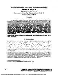
3 see Figure 1-1. This tooling configuration should promote preferential MR from the high points of the MSF features, and ultimately reduce the magnitude of the errors.
Figure 1-1 Fiber tool concept; (a) globally compliant (b) locally stiff To best of the author’s knowledge, this work is the first implementation of fiber based tools in a precision polishing application. This dissertation outlines the material removal mechanics of these tools whereby key process parameters and their impact on the polishing outcomes are identified. A finite element (FE) based foundation to assist in future tool design is introduced. Most importantly, it is demonstrated that these tools have the potential to reduce preexisting MSF errors. Chapter 2 provides a broad background about finishing processes in optics manufacturing. The focus of the discussion will be on freeform and aspherical component fabrication. Examples of their wide application in the industrial world will also be listed. Information will be provided regarding optics specifications and available mathematical tools for the characterization of these components. This discussion will have a special emphasis on the MSF’s and their impact on the optical performance. In chapter 3, the initial steps in design, fabrication, and characterization of fiber based tools are described. Two different approaches, experimental and FE simulations, are
4 employed to reach this goal. Fiber types qualified by both the experimental test bed and the FE model are used in the fabricated fiber based polishing tools. Chapter 4, contains details on the polishing tests conducted on planar BK7 glass samples. The test results in this section demonstrates the ability of these tools to remove material from glass under different testing conditions. The main process parameters impacting the polishing outcomes (MR rates and surface finish) are identified. An understanding of the fiber – abrasive – workpiece interaction is introduced. Chapter 5 scopes a more practical perspective; integration of the tools into a commercial 5 axis polishing machine and the resulting challenges. These issues include, long term polishing response of the tool, as well as its performance near the edge of the workpiece. The stability of the tool’s material removal footprint over long polishing runs is investigated. Lastly, initial testing results on non-planar samples will be presented. These tests took place onsite OptiPro Systems located in Rochester, NY. In Chapter 6, the ability of fiber based tools to reduce MSF features is demonstrated. This chapter includes results with respect to the reduction of MSF features from planar surfaces under different testing conditions. An additional two-step FEM is introduced, to assist the identification of fibers suitable of reducing MSF features. The same model is used to explore the design of alternative novel fiber geometries. Examples of alternative fiber geometries with potentially higher efficiency in reduction of MSF features will be illustrated. In the final chapter, chapter 7, the work is summarized and directions for further development of fiber based tools are discussed.
5
CHAPTER 2: LITERATURE REVIEW 2.1 Polishing optical components 2.1.1 Ancient era It is believed that the first optical components made by mankind were polished mirrors about 8000 years ago in Çatal Höyük [1]. Çatal Höyük was located somewhere in the central southern modern Turkey [2]. The first polished lenses are dated back to 2575 BC (before Christ), in ancient Egypt. Their purpose mainly were to serve as ornaments on the Egyptian statues [1]. Primitive polishing mostly involved the use of stones rubbed against the target surface. The polishing agents were usually water or some kind of oil based fluid. 2.1.2 Modern era In the contemporary optics industry, hard and brittle materials are abound. Grinding is usually the main process to shape the part as close to its final figure. However, the grinding process is very aggressive, and the part produced as such, will have a matt finish. Polishing, is used as a proceeding step, where quality, and specular surfaces can be produced. The mainstream polishing tools, in the modern times, is a layer of a polymeric pad or pitch material adhered to a rigid substrate, sometimes via an intermediate supporting material, e.g. foam, rubber, etc. This intermediate layer is used to control the flexibility of the polishing tool. The polishing agents used are typically a slurry containing fine abrasive particles (usually < 1 µm).
6 2.2 Conventional Optics vs Freeform and Aspherical Optics Optical components are largely divided into two groups. The first group are the more conventional optics with constant radius of curvature (ROC) over their entire clear aperture (CA), i.e. planar and spherical optics (Figure 2-1 left). The CA of an optical component refers to the functional region of the optic. The more modern optical components are optics with variable ROC across their aperture. Aspherical optics are a group of such optics that possess at least one axis of rotational symmetry. Freeform optics, contrary to aspherical optics, have typically no axis of symmetry and they, too, have varying ROC over their aperture (Figure 2-1 right).
Figure 2-1 Planar and spherical optics vs aspherical and freeform optics Planar and spherical optics have been manufactured from approximately the beginning of the 18th century in large numbers and even to-date are widely used as the main ingredient in optical systems. One main flaw of the spherical optics is the inherent third order spherical aberrations induced by such optics. These errors are typically compensated by the use of multiple components within the system. The first use of an aspheric lens in an optical system can probably be attributed to Francis Smethwick (late 17th century) [3], in which he uses “not-spherical” glasses in his telescope and burning glasses. The term “Aspheric” seems to be coined around 1922 [4].
7 Although aspherical optics and conics were commonly used, prior to the 70’s, easy production of such optics was nearly nonexistent. The reason for that is while fabrication of tools with constant ROC’s was relatively easy, the varying ROC of the aspheres caused a lot of problems during the polishing for the aforementioned rigid tools. After the 70’s emergent manufacturing, computational, and metrology capabilities promoted the use of aspheres in a wide range of industrial applications. Automotive headlighting, high power diode lasers, imaging optics, UV and EUV lithography projection lenses [5, 6] are just a few examples of systems that use aspherical optics. The main advantage of using an aspherical surface is to decrease/control the spherical aberrations, of an optical system with less components needed [7]. The application of freeform optics is more recent than aspherical optics. Jian et al. [8] have classified these surfaces into three distinct groups; (1) freeform surfaces with “steps, edges and facets”, e.g. a Fresnel lens, (2) freeform surfaces containing “tessellated patterns”, e.g. road signs, and (3) smooth freeform surface which lacks any steps, edges, or tessellated patterns. The term “freeform” used henceforth, refers to smooth surfaces that exploit the freeform shape. The first use of a freeform surface in an optical application can probably be attributed to Luis Alvarez. In the 1960’s Alvarez came up with a design of optical lenses where their surfaces can be described in terms of third order polynomials. The use of two identical lenses with the prescribed surface can provide the system with a variable spherical power [9]. With the advances in the CNC machining and positioning, the implementation of freeform optics in optical systems design increased significantly [10]. The first commercial adoption of a freeform optical surface is attributed to the Polaroid SX-70 camera [10-12]. Freeform optics find application across the entire optics
8 industry. From imaging optics, e.g. in wide FOV mirrors and overhead displays, to illumination applications, e.g. high brightness LED’s [11]. Figure 2-2(a) shows the application of freeform optics in the illumination optics of a gas station. The freeform optics used in this gas station have enabled a much more focused light. Figure 2-2(b) depicts how a freeform mirror can greatly enhance the FOV of a car side mirror.
Figure 2-2 (a) Application of freeform optics to the illumination of a gas station [13] (b) application of a freeform mirror in a car side mirror [14] 2.3 Polishing Configurations The polishing process is comprised of a polishing tool, workpiece, and polishing slurry carrying abrasive particles. The polishing is occurred as a result of the interaction of the three aforementioned components, through abrading material off the workpiece surface. In the modern industrial world, a layer of a polymeric pad [15] or pitch-based [16] material is adhered to a rigid substrate, comprising a polishing tool. The tools are used
9 commonly in two different configurations, known as full and sub aperture polishing configurations. 2.3.1 Full-aperture polishing The full-aperture polishing configuration (Figure 2-3(a)) is where the polishing tool is larger than the workpiece, and ideally the ROC of the end product will be the same as the ROC of the polishing tool. As it can be seen the entire workpiece remains in contact with the polishing tool over the course of the process. This configuration is mostly limited to fabrication of parts with constant ROC i.e. planar and spherical optics. Yet there are quite a number of notable full-aperture approaches developed by different researchers that have shown promise in manufacture of slow aspherical optics, i.e. aspheres with small departures from sphericity (smaller than 80%). The first published method can be attributed to David Brown, where he polishes the Herchel Telescope mirror with a special full size lap [17]. He uses a structured lap which offers passive bending and as a corollary this configuration assists the tool in removing undesired distortions from the aspherical mirror of the telescope. Later Jacob Lubliner and Jerry Nelson and their coworkers [18, 19] introduced the stressed mirror polishing method for the fabrication of off-axis paraboloid mirror segments of the 10 m telescope of University of California [20]. In this technique, the aspherical mirror segments are stressed as such that they are made to take the form of a sphere. Conventional spherical polishing is then used iteratively to produce the end product. Releasing the part post the process will restore the aspherical shape of the optic. Beckstette et al., [21] developed the use of a flexible rectangular large lap where the load on different zones of the tool is adjusted via actuators to accommodate the aspherical variable ROC. The tool consists of a thin layer responsible for holding the polishing pitch
10 i.e. “membrane polishing”, and a set of actuators applying adjustable pressures on this thin layer. Finally, the use of a “stressed lap” in the University of Arizona was adopted by a group of researchers [17, 22, 23]. This polishing configuration consists of a rigid polishing lap which continuously bent by controlled forces to conform to the aspherical shape of the optic. Even though many researches have investigated the influence of the process parameters on the polishing outcomes, to make the end product of such a polishing configuration predictable and capable of producing high quality and accurate geometries, accomplishing such surfaces with this type of polishing requires highly skilled opticians.
Figure 2-3 Polishing process configurations; (a) full-aperture polishing (b) sub-aperture polishing 2.3.2 Sub-aperture polishing In this setup, the polishing tool is downsized to dimensions smaller than the workpiece (Figure 2-3(b)). The tool is only in contact with a portion of the workpiece and is translated on a given path removing material as it goes. The advantage of this configuration is that the smaller tools have the ability to manufacture variable ROC on the
11 surface workpiece. This is achieved by combining the tools dwell time at any point on the surface with knowledge of the tool’s MR (see section 2.5 for additional details) Three main issues arise due to the nature of the sub-aperture processes; (1) potential curvature mismatch between the tooling and the workpiece on a localized scale, (2) tooling roll-off effects near the edge of the workpiece, and most importantly (3) inducement of mid-spatial frequency errors due to the remnant tool path marks.
Figure 2-4 (a) Tool and freeform workpiece curvature mismatch (b) uneven pressure distribution of tool near workpiece edge The curvature mismatch is only a difficulty when dealing with optics that exhibit very high local variations of the ROC. Figure 2-4(a) demonstrates this issue. In conventional polishing, the so called “edge roll-off”, refers to the much larger material removal from the workpiece edge, due to uneven pressure distributions, see Figure 2-4(b). This is caused by the tool moving off the edge, thereby shrinking the contact area significantly, and as a consequence the rise of very high contact pressures [24, 25]. The third disadvantage associated with this polishing configuration, i.e. inducement of MSF errors, will be discussed later in section 2.6.3, but is related to remnant tool path marks inherent in the process This polishing setup is the most modern version of polishing systems and will be discussed in more detail in section 2.5.
12 2.4 Polishing Components and the Physics of Material Removal Polishing is an abrasive process where at its basic core, the workpiece, the tool, and loose abrasive particles are the main components of the process. The interaction of the three components leads to the removal of material from the workpiece surface. The polishing process, sometimes referred to 3-body abrasion process, and a close up of the described components is depicted in Figure 2-5(a), (b).
Figure 2-5 (a) Polishing process overview (b) close up of the 3-body interaction One of the first predictive models for polishing was proposed by Preston [26] in 1927. This model simply states that the material removal rate (MRR) is a function of the applied pressure on the abrasive to the surface of the workpiece and the relative velocity of the abrasive particle with respect to the workpiece. While this model overlooks a large group of parameters affecting the material removal (MR), Preston concludes that all these factors can be grouped into one constant, Kp (i.e. Preston’s Coefficient) with the assumption that the constant will not change, if no other parameter, e.g. particle type, slurry pH, temperature, etc., changes. Preston’s equation is used ubiquitously in the polishing research work to date and is as follows:
13 M RR = Kp P V
[µm3 /s]
(2-1)
AAACKXicbVDLSgMxFM34rPVVdekmWARxUWfahXUhVNwIIlSxKnTGkklv29AkMyQZoQzzPW78FTdd+Nr6I6a1gq8DgcM593BzTxhzpo3rvjpT0zOzc/O5hfzi0vLKamFt/UpHiaLQoBGP1E1INHAmoWGY4XATKyAi5HAd9o9H/vUdKM0ieWkGMQSCdCXrMEqMlVqFIz+ELpMp4awrd7Ozi4vD01YaZ7iOr7Df0zGhkFaEyHDTFwkWt5U9Hfgg21+JfKtQdEvuGPgv8SakiCaotwpDvx3RRIA0lBOtm54bmyAlyjDKIcv7iQa7tk+60LRUEgE6SMenZnjbKm3ciZR90uCx+j2REqH1QIR2UhDT07+9kfif10xMpxqkTMaJAUk/F3USjk2ER73hNlNADR9YQqhi9q+Y9ogi1Nh2RyV4v0/+Sxrl0kHJOy8Xa9VJGzm0ibbQDvLQPqqhE1RHDUTRPXpET+jZeXCGzovz9jk65UwyG+gHnPcPjBemRg==
The MR mechanism of polishing is a very complex chemo-mechanical process. Understanding the MR mechanism of polishing has been the subject of a vast number of research articles in the past. Evans et al [27] have provided an excellent and detailed review of the different possible removal mechanisms during polishing. Figure 2-6 depicts a summary of the removal mechanisms detailed in [27].
Figure 2-6 Possible material removal mechanisms during polishing [27] The initial MR mechanism theories mainly attributed the polishing MR to abrasion action of the abrasive particles on the surface. It was speculated that the applied pressure on the abrasive particles causes the appearance of a groove on the surface which is thought to be a result of mechanical ploughing and/or cutting. Sir Isaac Newton [28] was one of the first proponents of this model. Samuels [29] provides evidence of this removal mechanism by showing SEM imaging of polished metals and the residue swarfs of material that greatly resemble grinding chips.
14 Later, in the early 20th century the “flow hypothesis” became very popular. Sir George Beilby [30] is probably one of the first scientists who proposed this model. According to this hypothesis, the local heat generated as a result of the friction between the abrasives and the surface, softens the surface material, leading to the plastic deformation of the affected zone. The deformed material is moved to the openings in-between the asperities of the surface, resulting in a smoother and specular surface, as expected in polishing. The chemical aspect of the removal mechanism describes the formation of an affected layer, the “gel” layer, on the surface of the workpiece as a consequence of the chemical reaction between the slurry fluid and the workpiece surface. Harada and Izumitani [31], have shown how the different chemical combinations of polishing slurries on glass changes the micro-vickers hardness of the glass surface. The adhesion of the formed gel layer to the abrasive particles and/or the mechanical ploughing action of the abrasives on this softer layer causes the removal of material. Finally, the concept of “chemical tooth”, was introduced to explain the removal mechanisms that weren’t otherwise explainable with the mechanisms described in the preceding paragraphs. In this description of the MR mechanism, the chemical bonding between the abrasive particle and the surface of the workpiece in the microscopic level is the main cause for the removal of material off the surface of the workpiece. The chemical reaction of the abrasives is speculated to be enforced near zones with defects on the surface of the glass. This mechanism, best explained by Cook and Brown [32, 33], captures the chemo-mechanical nature of polishing comprehensively. In this description provided by Cook [32] the chemo mechanical nature of MR has five key stages; (1) the water diffusion
15 under the glass surface, (2) the glass surface dissolving in water under the polishing pressures (3) the chemical bonding of the dissolved glass material to the abrasive particle, (4) the dissolved material can back-deposit on the surface under special condition which this affect the MRR, and (5) the dissolution of the surface as a result of interaction between the particles. Ed Paul [34] has proposed a generic predicting model that encapsulates the chemo mechanical nature of the polishing based on Cook and Browns description. The application of this model to polishing tungsten [35] has shown a good agreement between the experimental and that predicted by the model. The polishing was done under a variety of chemical and mechanical parameters. More recently, Suratwala and his group [36-38] in Lawrence Livermore national lab (LLNL), have extensively provided invaluable insights in the application of Cook and Brown model in polishing glass. Their investigation has revealed the impact of slurry chemistry, abrasive size, pad stiffness, pad texture, on the glass polishing rates. In summary of this section, Cook and Brown material removal mechanism is the most widely accepted description of the polishing process and many other researchers have provided evidence that supports their theory. While the MR mechanism theories presented in this section were brief, the goal was to indicate the complexity of the apparently simple polishing process. The focus of this work was not to advance any additional MR mechanism theories, but rather applying general conventions to the process developed in this dissertation.
16 2.5 Deterministic Finishing Deterministic finishing, refers to a process whereby the final geometric form of the optic can be predicted within low associated uncertainties. The sub-aperture polishing tooling as well as great advances in computer technology and fast, digitized quantitative measurement of optics, has made deterministic finishing possible. Over approximately the past fifty years a variety of technologies were developed that could be used as a MR tooling, in a deterministic fashion. Most of the technologies rely on the abrasive processes in removing material. the most notable are listed in Table 2.1 All deterministic finishing processes require a stable removal footprint. The tool removal footprint per unit time while stationary, is known as the tool influence function (TIF). The TIF changes with variety of process parameters, e.g. workpiece material, polishing slurry, tool type, process kinematics, etc. [39]. Better measurement and characterization of the TIF yields better predictability of the process outcome and thus a higher process determinism [40].In each process a tool path is generated, i.e. the tool is rastered over the entire surface The tool can dwell at each point of the tool path as much as needed, longer dwell times result in higher MR at that point. A matrix containing the dwell time of the tool per point, i.e. the dwell time matrix, is calculated by mathematical deconvolution between the total amount of MR desired from the part and the TIF. The desired MR from the workpiece is determined by subtracting the ideal surface map from the measured (actual) surface map. The described process chain is iterated until the optic meets its specifications, see Figure 2-7.
17 Table 2-1 Deterministic finishing processes Mechanism Year Process name
Tool Type
Limitation
Pad tool
Rigid tool
Pad tool
Rigid tool
Computer assisted optical surfacing Abrasion
1972 (CAOS) [41] Computer
Abrasion
controlled
optical
1977 surface (CCOS) [42, 43]
Float Abrasion
1980 Float polishing [44]
Low MRR polishing
Canon Abrasion
super
smooth
polisher
1991
Pitch tool
Rigid tool
(CSSP) [45] Magnetorheological Abrasion
finishing
1995
Complex MR fluid
(MRF) [46-48]
tooling
Abrasion
1998 Fluid jet polishing (FJP) [49, 50]
Abrasive jet
Sensitive TIF
Abrasion
2002 Precisions [51, 52]
Bonnet tool
Rigid tool
MR fluid jet
Sensitive TIF
Ion beam
Low MRR
Magnetorheological Jet® (MR jet) Abrasion
2006 [53, 54]
Ablation
1989 Ion beam figuring (IBF) [55]
Atomic Elastic level
emissions
machining Rotating
1987
Low MRR (EEM) [56, 57]
sphere
removal Chemical
Chemical vaporization machining Plasma 1992
Etching
Low MRR (CVM) [58]
beam
18
Figure 2-7 Deterministic finishing process map The technologies in Table 2.1 mostly focused on alternative finishing tooling that could be incorporated in a sub-aperture system and would offer specific advantages. Walker et al. [59-61] developed the use of the “bonnet” polishing tool in the “Precision’s” process, see Figure 2-8(a). The machining center used for this tool, the Zeeko machine, provides 7 axes of motion, enabling the orientation of the tool in different angles. The Zeeko polishing system’s high yield and the ability to produce low surface roughness values, has made this system one of the most widely used machines in the optics industry.
Figure 2-8 (a) Bonnet polishing tool [62] (c) MRF system [63]
19 One of the other most commonly used and efficient deterministic systems today was developed in the 90’s, the QED magnetorheological finishing (MRF) system [64]. Kordonsky et al. [46] demonstrated that a stiffened ribbon of abrasive rheological fluid under the influence of a magnetic field and brought into contact with an optic surface, causes the removal of material from the part. This idea was transferred into a sub-aperture polishing apparatus where the fluid ribbon is carried on top of a rotating wheel [47, 65]. The TIF of the process, is basically the material removal profile of the MRF where the fluid contacts the optic and removes material, see Figure 2-8(b). Achieving figure error tolerances less than 30 nm and surface finishes of the order of 1 nm RMS, with the MRF system is very feasible. The material removal mechanism of the MRF process is mostly attributed to the fluid shearing the surface through the abrasive particles [66, 67]. In each of the sub-aperture processes, the integral components are, integration of the measurement data into the process, a stable tool TIF, as well as controlled motion of the tool, including the translation feed and spindle speeds. These processes, enable the optical fabricators to easy produce freeform and aspherical optics. That being said, a remaining unsolved challenge with respect to optics fabricated by deterministic finishing is the MSF errors imparted by the processes, see section 2.6.3 for details on MSF errors. 2.6 Surface Characterization of Optical Components Researchers active in metrology and characterization of engineering surfaces, typically seek to measure and evaluate surface geometrical properties, as well as, their mechanical properties. This dissertation, however, doesn’t consider the processed surfaces in terms of their mechanical behavior. The concepts laid forth for quantification of surfaces will be described from the optician’s perspective, i.e. with respect to dimensional
20 metrology. One common approach for characterization of the dimensional errors of surfaces, is the separation of the surface components into three different regimes. In general these three regimes are termed as “form”, “waviness” and “roughness” [68, 69]. Though defining sharp distinguishing lines between the aforementioned errors is usually challenging, as the distinguishing lines are dependent on the application of the surface. In case of an optical component the wavelength of the incident light will be a determining factor. Figure 2-9 illustrates these three components for a given “planar” workpiece.
Figure 2-9 (a) Form, (b) waviness and (c) roughness errors for a “planar” workpiece 2.6.1 Form or figure Form or figure refers to geometrical features of the surface that can be described with periodic functions with periods typically larger than 3 mm. Figure error is usually caused by the large mechanical deformations induced on the workpiece during the mechanical processing of the part. The mechanical deformations can be caused by the residual stresses present in the part, either from previous processing, and/or the fixturing of the workpiece during the process. The other sources of figure error can be the thermal variations during the process.
21 Figure error causes the input wavefront of a lens to distort in an undesirable way, see Figure 2-10(a). A close up of the surface geometry and its ideal shape is depicted in Figure 2-10(b). The transmitted wavefront remains relatively coherent, therefore, it is expected for the optic to be able to form an image with present distortions. This type of distortion/aberration is different than that of inherent to special optical geometries, where the correction of such aberrations can be done with subsequent optical elements. Detailed discussions on how optical designers use different approaches for the correction of common
inherent
aberrations
are
available
in
many
sources
[70-72].
Striving for fabrication of lenses with low figure errors, as the underlying system structure could always facilitate the design process, as attention is only needed for fixing the inherent optical aberrations.
Figure 2-10 (a) The influence of figure on a planar wavefront, (b) close up of the surface geometry and the extent of figure error In optics, it is common to describe figure errors via a set of orthogonal base polynomials. The RMS of the base polynomials and/or the peak to valley (PV) of each
22 individual term is used to specify the form errors for a given optic. There are a variety of these polynomials developed by mathematicians over the past century. Since circular parts in optics are prevalent, using a set of orthogonal polynomials in the polar coordinates can facilitate the characterization of a large group of optics. One of the most widely used orthogonal basis, was first derived by Frits Zernike [73]. A detailed account of the Zernike polynomials and their relevant shapes can be found in reference [74]. Zernike polynomials ought to work very well in characterization of conventional optics, and theoretically it is possible to use them for describing freeform and aspherical optics. However, as pointed out by Forbes and Kaya [75-77], the use of Zernike polynomials per se is not numerically efficient. Forbes showed that the use of a proper basis for the orthogonal polynomials can significantly improve characterizing aspherical optics in his paper published in 2007 [75]. The International Organization for Standardization (ISO) has provided documentation for specification of form in optical drawings in the ISO 10110 parts 5, 12, and 19 [78-80]. The part 12 and 19 are recommended for specifying aspherical and freeform optics respectively. 2.6.2 Roughness or finish Surface roughness or finish, is a term used to describe surface features that are repeated with a much smaller period than that of form. The upper limit of roughness bandwidth is considered ~ 0.08 mm for visible light applications. The roughness of a surface post of a process is highly dependent on the mechanical and chemical aggressiveness and the MRR of the process. Mechanically Aggressive and high MRR processes such as grinding produce matt finishes. Whereas, slow processes like
23 polishing can produce specular and shiny surfaces. Polishing under favorable chemical conditions and the absence of etching typically leads to surfaces with low roughness values. The surface roughness of optical components causes the incident light to scatter in random directions. That is mainly due to the comparable lateral dimension of surface finish to the wavelength of light. The random direction of the scattered light implies that for roughness values above a certain limit no image can be formed by the optical component, which is contrary to the impact of figure error. For a specular surface (which are desired for most optical applications), the amount of scattered incident light is directly correlated to the square of the RMS of the surface roughness [81-84]. The well-known Rayleigh-Rice theory introduces the expression for the correlation between the distribution of scattered light and surface roughness. The total integrated scatter (TIS), which provides a measure of the number of scattered photons in the optical component, is directly correlated to the RMS of the surface roughness with the following relation given by Harvey et al [85]: T IS ⇡ 4⇡ /
2
(2-2)
Where s is the RMS of the surface roughness and l is the wavelength of the incident light. Based on the argument above, for quantification of surface roughness on optical surfaces, the RMS of the high frequency surface deviations is used. To quantify the high frequency surface variations, a high magnification interference microscope can be used. For separation of the local forms of the measured data, high pass filtering is applied. These filters are, nowadays, available in digital format and is applicable to the digitized measured data. The application of digital filtering to the measured data is detailed in many highly regarded works [68, 86]. As suggested by the aforementioned references the use of the
24 discrete Fourier transform (DFT), and suppression of the unwanted spatial frequencies present within the data can be conveniently implemented, to separate the roughness data. The part 8 of the ISO 10110 standard is dedicated to the specification of surface texture on optical components, which is inclusive of the surface roughness as well [87]. The standard recommends the use of the RMS of the roughness for optics specification. The definition for the RMS of the roughness data is provided in ISO 25178-2 [88].ISO has also, disseminated documentation which elaborates on the different type of filters and their operation on the surface data [89-92]. The afore mentioned standards recommend a cutoff of 0.08 mm for the calculation of surface roughness. 2.6.3 Waviness or mid-spatial frequencies (MSF) Waviness, or MSF refer to the surface features that have a spatial period of approximately 0.08 mm up to 3 mm. As can be inferred by the number, the MSF wavelength is in-between the scale of features associated with form and roughness errors. The main source of the inducement of MSF errors is the tool marks post a subaperture process. Since the tool path in the sub aperture processes are a raster path or a spiral path, the periodic MSF features are induced with a period correlated to the path stepover. Hull et al [93] have provided a list of the possible sources of MSF errors. Some of the most notable ones due to the fabrication process are: (1) the imprint of the structure ribs of backing of the optic if a light weighted structure is used (2) poor tool and workpiece curvature mismatch and uneven pressure distribution of the tool over the aperture of the workpiece, (3) imprint of the tooling back support structure on the surface. The growing interest in use of freeform and aspherical precision optics, and the more use of sub-aperture processes as a corollary, has signified dealing with MSF features. Parks [94] has shown
25 how not considering the MSF errors can result in failure of the performance of the optic containing them. The existence of MSF features on an optic causes the appearance of flare in the image produced by such optics. This phenomena is attributed to the “small-angle scatter” [95, 96] effect of the MSF features. Small-angle scatter effects, spread the area of the point spread function (PSF). Based on the geometrical optics theory, a converging lens is expected to image a perfect point source to a “perfect” point. See Figure 2-11(a). Yet due to the limited aperture size in any lens (or optical system) the effects of diffraction prevent the system of achieving such a perfect point, see Figure 2-11(b). The intensity distribution of the imaged point source is the PSF of the optical system.
Figure 2-11 (a) “perfect” imaging of a point source (b) “real” diffracted spot image The effect of the different surface errors, figure, finish and MSF, on the PSF was investigated by Harvey et al [96]. Figure 2-12 shows linear profiles across the PSF of surfaces with figure, finish, and MSF errors. It is clear that the MSF errors, contrary to figure and finish broadens the PSF. Figure and finish on the other hand reduce the peak magnitude of the PSF.
26
Figure 2-12 The effect of figure, finish, and MSF errors on PSF [96] Figure 2-13(a), (b) show the spot imaging of two optics without and with MSF features respectively. As evident in the figure, the optic with MSF features (period of 2 mm and RMS of 35 nm), has a broader image of the point source. As a consequence of this broadening of the PSF, flare and reduction in the resolution of the optical system will occur.
Figure 2-13 (a) PSF of an optic with no MSF features (b) PSF of an optic with MSF features with a period of 2 mm and RMS of 35 nm For quantification of the MSF errors, the power spectrum density (PSD) of the surface deviations of the optic is one of the most widely used techniques in the optics community. Generally speaking, the PSD of the surface is obtained by applying the Fourier
27 transform to the surface height data. The MSF features, as pointed out earlier, are periodic surface features in nature. Therefore, the power spectrum should demonstrate a strong signal at the frequency of the MSF’s. The power of this signal can be translated to the magnitude of the MSF errors. This can be conveniently explained by the use of Parseval’s [97] theorem expressed below: Z AAACi3ichVFdaxNBFJ1dq22jttE++jI0CBUx7qYFU1EoiNDHFowt7m6W2cndZOjM7DJzVxK3+2v8R775b5wkW9C24IXhHs65X3NvVkphMQh+e/6DjYePNre2O4+fPN3Z7T57/tUWleEw4oUszGXGLEihYYQCJVyWBpjKJFxkV5+W+sV3MFYU+gsuSkgUm2qRC87QUWn3ZxzFQmNav3Eux0Uzrl+3iMaSmSlc/2jBwXztX90I4wGdzOlH+r8C324K5Gk9b+4psuJpPLMl41AfKtVEsaqoGh8mnTjppN1e0A9WRu+CsAU90tpZ2v0VTwpeKdDIJbM2CoMSk5oZFFxC04krC67VFZtC5KBmCmxSr5bZ0JeOmdC8MO5ppCv274yaKWsXKnORiuHM3taW5H1aVGE+TGqhywpB83WjvJIUC7q8DJ0IAxzlwgHGjXCzUj5jhnF091suIbz95btgNOgf98PzQe9k2G5ji7wg++SAhOQdOSGn5IyMCPe2vbfe0Dv2d/wj/73/YR3qe23OHvnH/M9/AFbDxjQ=
+1 2
1
|z(x)| dx =
Z
+1 1
|Z(fx )|2 dfx [µm3 ]
(2-3)
Where z(x) is the height distribution on a linear 2D profile, and Z(fx) is the Fourier transform of z(x). The Parseval’s theorem implies that the reduction in periodic surface errors, will translate into the reduction of the power of the aforementioned error in frequency space. The use of the PSD function for evaluation of surface roughness was first investigated by Rasigni et al [98]. In their paper they show that the spectral analysis can be used to compute the roughness and waviness of the surface with the PSD. Church et al [99] had used the PSD in comparing the measurement data of a single part using two different instruments. Nevertheless, it was Church and Tackas [100] that firstly demonstrated the use of the PSD of the surface measurement data can be very beneficial in prediction of the light scattering characteristics of the surface. Later the researchers in LLNL [101-105] published documents on how the PSD could enable imposing tolerances on the optics manufactured for the national ignition facility (NIF) optics. Some efforts for the use of the aerial PSD has been taken more recently [106, 107]. However, little usefulness of this method has been showcased thus far. One of the other metrics common in determining the image quality of an optic influenced by the MSF features is the use of modulation transfer function (MTF). The MTF can be quantified by evaluating the square of the absolute value of the Fourier transform
28 of the PSF. Intuitively speaking, the MTF is the power spectrum of the PSF and it reveals the resolving power of the optic for a given feature size. The MSF errors cause the MTF values to be smaller at higher spatial frequency features. For more details of the effect of MSF errors on the MTF look into references [96, 108, 109]. The ISO 10110 standard [110] has instructions on specifying the PSD tolerances on optical drawings as a method in controlling MSF specifications on optical components. 2.7 Available Solutions for MSF Reduction MSF errors are bearing significant amount of limitations on the optical components containing them. The removal of the MSF errors, post the processes causing them, is also very costly and challenging. Unfortunately, there are not many options available for the reduction of MSF errors on freeform and aspherical optics. For planar and spherical optics, a full-aperture tool with a hard polishing pad is usually used, see Figure 2-14. Parks and Evans [111] have conducted experiments using a conventional polishing tool, with backed foam of pellon to show preferential material removal from the high regions of the diamond turning marks from diamond-turned electroless nickel and aluminum.
Figure 2-14 Polishing MSF errors; (a) from planar (b) from spherical workpiece
29 The rigid full-aperture tooling cannot be used for polishing MSF’s off freeform and aspherical optics generally. The full-aperture tooling is mostly available for polishing MSF’s off parts with constant ROC, i.e. planar and spherical optics. Limited full-aperture MSF reduction technologies for aspheres are available. The VIBE polishing process developed by Optimax [112, 113] is a full-aperture polishing tool for removal of MSF’s from aspheres, see Figure 2-15. In this method, a rigid polishing lap with a flexible pad is used. The lap has dimensions as close as the aspherical workpiece. High frequency vibrations are applied to the lap during the polishing which assist in removing the MSF errors. The lack of any rotational symmetricity of freeforms rules out any possible full aperture solutions for the removal of MSF’s of such optics.
Figure 2-15 Optimax VIBE finishing process [113] The other group of approaches for controlling the extent of the MSF errors is modification of the polishing tool path. The typical tool path for polishing freeforms are shown in Figure 2-16. Some control over the wavelength of the induced MSF errors can be applied by modifying the tool stepover in each case [114].
30
Figure 2-16 Conventional polishing tool paths The use of “pseudo random” polishing tool paths by Dunn et al [115] has shown to decrease the amount of MSF errors. Figure 2-17(a) shows this pseudo random tool path. Wang et al. [116] have adopted a similar approach by creating polishing tool paths in “unicursal random maze” configuration, Figure 2-17(b). Toolpaths with non-conventional shapes, and not random in nature, are also investigated by a few researchers. The use of Hilbert tool paths, see Figure 2-17(c), in works by Dong et al [117] and Wang et al [118] has shown success in achieving MSF errors with less severity than that achievable by conventional tool paths. Essentially the idea is to intersect the polishing tool paths randomly ensuring that no periodic features with a constant wavelength is produced. The existence of uneven pressure distributions of the polishing tools, nonetheless, is unavoidable. While the tool paths can greatly aid in smoothening of the MSF errors on parts with mild slope variations, the case is far more complicated for steeper optics.
31
Figure 2-17 Non-conventional polishing tool paths; (a) pseudo random tool path [115] (b) Hilbert path and modified Hilbert path [118] The final group of methods for dealing with MSF errors on optics are alternative sub-aperture tooling, that provide local stiffness to the MSF errors by some means incorporated in the tool architecture. It also should enable the tool to accommodate for the various ROC that are traversed over during the polishing action. Achieving the combination of the two is of great challenge. Dong et al [119] have developed a polishing tooling that resembles a discretized polishing pad tool, called “fixed abrasive diamond pellet (FADP)” tool, see Figure 2-18 (a,b).
Figure 2-18 The FADP tool [119]; (a, b) planar and spherical tool configuration (c, d) pre and post the removal of MSF errors
32 The segmented pellets in the FADP tool gives the relative compliance to the tool, yet the stiff nature of each pellet (~ 3 mm in diameter), enhances the tool rigidity on a local scale, and thus enabling the removal of MSF errors. The shortcoming with this method is clearly that optics containing small ROC’s cannot be polished and processed. Another method that researcher in LLNL [120] have shown to have potential in removing MSF errors off aspherical samples, is the use of float polishing. The float polishing apparatus was first introduced by Namba [121]. This polishing system is based on the principles of hydrodynamics. A thin layer of slurry fluid between the workpiece and the rotating precision machined lap, causes the particles to remove material off the surface of the optic, see Figure 2-19. This approach is very effective for low departure aspherical optics. The hydrodynamics with steeper samples and/or freeform shapes will become exponentially complex in such apparatus. Needless to say, the higher capital cost associated with this system is another limitation that should be mentioned.
Figure 2-19 Float polishing [122] (a) schematic, (b) machine in action In summary of this section, it is undeniable that a major vacancy of a technology for dealing with MSF errors on freeform and aspherical optics exist. The methods described here have a very limited scope and, in some cases, are specific to one specific geometry. This gave the motivation to adopt a more generic tool that would enable processing optics
33 with wider range of geometries. It is believed that the use of fibers can address the issue and successful implementation of a tool made of fibers can greatly enhance the capabilities of the optics manufacturing community in fabrication of freeform optics. 2.8 Summary In summary, polishing plays a pivotal role in modern day optics manufacturing industry. Yet, the mainstream polishing systems for finishing freeform and aspheres suffer from inducing MSF errors. These errors have limited the applicability of the optics to longer wavelength region of the electromagnetic spectrum. Today, scientists such as Parks, Evans, Nelson, etc., mostly agree establishing local stiffness to the higher regions of the MSF errors, is key to effectively reduce these errors. Several group of technologies, have shown success and potential in reducing the MSF errors and were described in this chapter. However, these methods mainly encompass a limited range of part shapes. With the great advances in computer science, optical systems design has moved at a very high pace. Successfully achieving MSF reduction of freeforms will aid in transitioning the freeform design into the visible light regimen, where it can have enormous impact. This requires the manufacturing industry provide methods of reducing preexisting MSF features. The work detailed in the following chapters seeks to address this issue.
34
CHAPTER 3: FIBER TOOL DESIGN, FABRICATION, AND TESTING 3.1 Introduction This chapter details three key topics with respect to fiber based tools design, fabrication, and characterization; (1) the key fiber metrics and fiber selection criteria are introduced (2) fiber metrics are measured and quantified using an experimental test bed, (3) initial tool designs and tool fabrication step are detailed, and (4) a finite element model (FEM) of the fiber workpiece fundamental interaction is created. 3.2 Fiber Selection Criteria As discussed in Chapter 2, Preston’s equation is the most widely used quantitative model for predicting material removal rates (MRR) in polishing. Pressure and velocity are both mechanical aspects of the polishing process. The Kp coefficient represents all the other elements (either mechanical or chemical) affecting the material removal (MR). In the present study, the majority of the work is focused on the mechanical contributions of the different elements involved in the fiber based polishing process. To the best knowledge of the author, the use of fiber based tools in polishing precision optics had not been published in literature prior to this work and publications thereof. This imposed a great challenge in opting a direction for studying these tools. Hence, the baseline of the work was founded upon Preston’s equation. Based on this premise, the main fiber selection criteria were the following; (1) The fiber should be
35 capable of applying a pressure that is expected to result in MR, (2) the fiber should established a reasonably long contact length on the workpiece to ensure that the fiber is capable of spanning multiple MSF’s, (3) the fiber should be able to retain its contact with the workpiece when in motion and polishing the workpiece, (4) The fiber should be sufficiently large and robust for ease of fiber handling and tool fabrication and, (5) the final tool design should be such to enable a systematic study on the tool workpiece interaction. Thus, for keeping the action of a single fiber relatively independent from other fibers any fiber cross over in the tool was prevented. 3.3 Fiber Selection Test Bed A simple experimental test bed for evaluation of an individual fiber interacting with a planar surface was utilized. This test bed is shown schematically in Figure 3-1.
Figure 3-1 Fiber selection test bed (a) fiber disengaged, (b) fiber engaged The test bed consisted of a micrometer stage with a displacement range of 25.4 mm and a resolution of 25.4 µm in the z direction. The fiber attached to the stage is illustrated
36 in Figure 3-1(a). The stage was lowered to bring the fiber into contact with a high precision scale, OHAUS® Adventurer PRO® (resolution of 0.1 mg). The approximated load corresponding to different fiber positions was measured via this scale, Figure 3-1(b). The height which the loads were measured in this setup would correspond to the plunging depth of the tool (DZ) for the polishing experiment. The length of the contact made between the fiber and the scale was measured approximately using backlighting and a ruler placed behind the fiber. Figure 3-2 depicts the image of the setup studying the Nylon 6/6 fiber.
Figure 3-2 Fiber selection test bed examining the Nylon 6/6 fiber A range of fibers with different cross section geometries (circular, triangular, rectangular, etc.), different fiber materials (Polypropylene, Acetal Co-Polymer, Nylon 6/6, etc.), and different critical dimensions (0.2 mm to 3mm) were sourced. The fibers were sourced from different suppliers. Some of them were procured from chain hardware stores such as Lowes® and HomeDepot®.
37 Table 3-1 summarizes the evaluation of a range of fibers using the test bed. The fiber dimensions were measured with an optical microscope. The Young’s moduli of the fibers were not provided by the vendors. Table 3-1 Fiber evaluation summary results for fiber length of 37.5 mm
Material Polypropylene (Tfiber) [123] Nylon 6/6 (N66) [124] Polyurethane (PS) [123] Carbon fiber (CF) [125] Co-Polymer [123] Silicone (SF) [126] Co-Polymer [123] Polyethylene terephthalate (PET) [123] Carbon fiber (CF) [125] Unknown Ceramic [127]
Geometry and dimensions (mm)
Modulus (GPa)
Contact length (mm)
Contact load (N)
Estimated pressure (kPa)
1.2 side
1.5
11.4
0.39
31
Ø1.6
2.5
5.8
0.53
600
2 ´ 0.6
0.5
15
0.3
5
1 ´ 0.1
140
30
0.35
12
Ø1.4
1
4.5
0.75
1016
Ø1.3
0.001
25
0.03
1.4
Ø0.5
1
6.75
0.01
29.4
Ø0.22
3
7.25
0.005
10
3.0 ´ 3.0
140
0.5 ´ 0.25
N/A
Fiber failed Fiber failed
Fiber failed Fiber failed
Fiber failed Fiber failed
The modulus of each fiber in the table was approximated from values available in the literature. The pressures were calculated through dividing the total contact load by the measured contact length and approximate contact widths. The contact widths for the triangular and rectangular geometries were taken as the width of the fiber itself. These values for the circular geometries were approximated via the FEM, detailed later in this
38 chapter, are in the order of 10 µm (PET fiber), 50 µm (Copolymer Æ0.5 mm), and 150 µm (fiber diameter > 1 mm). In each case the fiber was evaluated under conditions for which would provide the longest contact length achievable. The first eight fibers in Table 3-1 successfully satisfied the conditions for qualifying to be used in a polishing tool. All of the eight fibers had a sufficiently long contact length as well as reasonable contact pressures. Polishing tests with these fibers was conducted, and the results of such testing can be found in Chapter 4. The bending stresses for the last two fibers in the table, exceeded that of their failure stress, thus causing the fibers to fail under the testing. These two fibers were disqualified for use in a polishing tool. While conventional polishing pressures are of the order of 20 KPa to 100 KPa [128, 129], some of the pressure values given in Table 3-1 are much higher. To decrease the fiber contact pressure, two conditions should be met; (1) decreasing the applied load, and (2) increasing the fiber contact length. Tilting the fiber relative to the tool axis accomplished both of the two aforementioned points. To enable the experimental test bed for evaluating fibers at a tilted position, a protractor for measuring the angles was accommodated on the testing setup, see Figure 3-1 and Figure 3-2. As a result of tilting the fibers to an angle where the pointer in Figure 3-1 was at 40°, 50% reduction to the estimated pressures listed in Table 3-1 was achieved. 3.4 Fiber Based Tool Design and Fabrication One of the main challenges of the work in its infancy was the vacancy of any prior work about the application of fiber based tools in precision polishing. This made the design space of such tools very enormous. Any arrangement of fibers basically, can be a different design. Regardless, the design opted for the majority of the work here was based on the
39 premises detailed in section 3.2, i.e. ease of fabrication and the ability of a systematic study of the fiber workpiece interaction. Figure 3-3 illustrates two initial designs used in the work. The first design, referred to as FT-1, Figure 3-3(a), was the tool configuration most used for the work in this dissertation. Basically, this configuration is very similar to a simple paint brush in which the fibers are parallel to the shaft of the tool. In the second design, referred to as FT-2, see Figure 3-3(b), the fibers are tilted at 40° with respect to the tool axis. This design is similar to the scenario where the fiber is tilted in the fiber study setup. The goal of this design, as mentioned thereof, was to decrease the total polishing pressure exerted by the tool.
Figure 3-3 Fiber based tool initial designs; (a) FT-1design (b) FT-2 design The tool head was fabricated by turning a piece of aluminum initially. For a typical tool, twelve holes, as fiber holders, were then drilled unto the tool head. The diameter of the drilled holes depends on the fiber used in the tool. The fibers are glued with Loctite® Super Glue in the holes. This facilitates later detachment of the fibers from the tool by submerging the tool into an acetone solution.
40 Figure 3-4(a) shows a fabricated tool using twelve Nylon 6/6 fibers with fiber length of 37.5 mm. The tool was lowered down towards the workpiece to establish contact between the tool and workpiece. Typical DZ values were based on results from the initial testing of the fibers on the fiber selection study setup. Upon contact with the workpiece, the fibers fanned out radially and created an annulus region in physical contact with the surface, see Figure 3-4(b). This tool was used for the majority of the polishing experiments throughout this dissertation.
Figure 3-4 Fiber based tool FT-1 design attached to the Bridgeport milling machine; (a) disengaged, and (b) engaged with workpiece 3.5 Fiber – Workpiece FE Modeling One of the main shortcomings of the fiber study test bed, was that, it doesn’t provide any insights on how the applied contact pressure by the fiber is distributed over the fiber-
41 workpiece contact length. For comprehending the fundamental fiber-workpiece interaction, a FE model (FEM) was created. The model is a static model (no tool rotation), created in ABAQUS®/Standard [130]. 3.5.1 Nylon 6/6 fiber While the FEM’s for different fiber material/geometry combinations were developed over the course of this work, details associated with modeling of a particular fiber is presented here. This fiber, the Nylon 6/6 fiber (sourced from Hahl-Pedex®: Hahl PA 6/6) (Table 3-1), was mainly chosen due to its extensive use in this work. The Nylon 6/6 fiber with a length of 37.5 mm and Æ1.6 mm was used. Elastoplastic behavior was attributed to the material of the fiber. The nonlinear behavior was accommodated through tabulated data obtained through the stress – strain curve shown in Figure 3-5. No additional creep behavior was included in the model.
Figure 3-5 Nylon 6/6 fiber stress/strain curve [124] 3.5.2 Glass workpiece The workpiece, made of glass, was only modeled using elastic elements. The modulus of elasticity was set as 70 GPa. The dimensions of the glass were taken as 37.5 mm ´ 5 mm × 1 mm.
42 3.5.3 FEM steps and boundary conditions To simulate the fiber-workpiece interaction a multi-step model was created. In the first step the fiber was bent in the plane of engagement (Figure 3-6(b)) by enforcing an angular displacement to the tip of the fiber. This deformation was necessary in the polishing experiment as well, for ensuring proper fiber-workpiece contact. In step 2 (Figure 3-6(c)) the workpiece was displaced towards the deformed fiber, until contact was initiated.
Figure 3-6 Fiber-workpiece interaction FEM steps Finally, in step 3 (Figure 3-6(d)), the angular displacement at the tip of the fiber was removed, while the workpiece was moved towards the fiber by a small amount (2 mm), causing the fiber to attain static equilibrium state, and establishing a full contact with the workpiece. The coefficient of friction between the surface and the fiber was taken as 0.1.
43 The normal contact behavior between the fiber and workpiece, was picked as “hard” contact. This implies that with the pressure contact approaching zero, the fiber will no longer be in contact with the workpiece [130]. Since the geometry of the FEM is symmetric, the model was halved in the plane of the fiber bending. The fiber is fixed at the top, where in the actual tool, reflects where the fiber is fixed to the tool head. The symmetry conditions were applied on the halved fiber and workpiece faces. The end of the fiber and the workpiece will observe boundary conditions in accordance with the model steps, described earlier. In step 1 and step 2, the fiber end was bent 120°, around the y-axis. This displacement was removed in step 3. For the motion of the workpiece, the displacement boundary condition was attributed to the bottom face of the glass plate. These displacements were 0 mm, 20.5 mm, and 22.5 mm, in step 1, step 2, and step 3, in the vertical direction respectively. The final displacement value was selected to reflect the DZ used in the polishing tests. 3.5.4 Meshing scheme and number of elements For discretization of the entire model, C3D10M (modified quadratic tetrahedral) elements were used. The fiber was meshed uniformly with element size of 100 µm. The glass workpiece on the other hand was equipped with biased meshing scheme. The element sizes were as small as 50 µm in the contact zone, whereas the mesh size far away from the contact zone went up to 5 mm. The total count adds up to 327,224 elements and 493,155 nodes. Figure 3-7 shows the overall meshing, as well as, the close up of the fine elements used.
44
Figure 3-7 Fiber and workpiece overall meshing and close-up of the finer elements 3.5.5 Model results (planar workpiece) As mentioned earlier, one of the main underlying parameters of the polishing process is the pressure distribution exerted by the polishing tool on the workpiece. Examination of the pressure distribution was a key goal of the FEM work. The experimental test bed explained in section 3.3 didn’t provide any insights on this distribution. However, the FEM can complement the experimental test bed providing fiber contact pressure distribution. This contact pressure distribution in ABAQUS is called CPRESS. Figure 3-8 shows the pressure distribution obtained from this model. A line profile of pressure (pressure on a line) was extracted from the centerline of the contact
45 zone, (Figure 3-8(b)), and a V-shaped profile was observed. This line was where the highest pressure values are exerted. The ability of fiber based tools in removing material will be discussed in detail in the next chapter, where it will be shown that the MR profile exhibits the same V-shape. The striking similarity between the removal profile and pressure profile, was indicative of two key points. First of all, this hinted that the MR of the tools most likely, obeyed Preston’s law of MR. In other words, the MR was directly correlated to pressure. Furthermore, it showed the potential of the FEM in predicting polishing outcomes of these tools. The FEA can be employed as powerful aid, in future fiber tool designs, as a consequence of the validity of the model.
Figure 3-8 Nylon 6/6 fiber-workpiece interaction FEM (a) contact pressure distribution (CPRESS), (b) pressure profile extracted from CPRESS along the dashed line Figure 3-9(a) shows the pressure distribution of the same Nylon 6/6 fiber, tilted at 40°, on a planar surface. The pressure profile from the centerline of the pressure distributions is illustrated in Figure 3-9(b). The pressure profile suggested that tilting the fiber had indeed reduced the maximum contact pressure. The MR testing results of this tool is presented in Chapter 4 as well.
46
Figure 3-9 FEM of the tilted Nylon 6/6 fiber at 40° (a) contact pressure distribution (CPRESS), (b) pressure profile extracted from CPRESS along the dashed line As it will be discussed in Chapter 6, the FEM lays the foundation for selection of fibers that promote higher MSF removal capability. 3.5.6 Model results (non-planar workpiece) A similar FEM procedure to the one described above was used to model the fiber – workpiece interaction on a curved surface. The fiber was modeled with the same specifications detailed in the previous subsection. The workpiece was Æ75 mm concave surface with ROC of 75 mm. To minimize simulation time, only an arc of the spherical workpiece was created in the FEM. The same idea of halving the fiber along its line of symmetry was employed. The C3D10M elements were used for the discretization of both fiber and the workpiece. a total 256,834 number of nodes and 166,952 number of elements were created. Figure 3-10(a) shows the engaged fiber with this workpiece as well as the contact pressure distribution of the fiber on the workpiece. Depicted in Figure 3-10(b), the pressure profile obtained from the FEM suggests that the width of the pressure profile is
47 narrower than that of the planar surface. Yet the profile has the same V-shaped geometry. Testing on this sample will be done in Chapter 5.
Figure 3-10 FEM of the Nylon 6/6 fiber-concave workpiece interaction; (a) contact pressure distribution (CPRESS), (b) pressure profile extracted from CPRESS along the dashed line 3.6 Summary In summary of this chapter, initial steps in design, fabrication and characterization of fiber based tools were taken. The key highlights of this chapter were the following: •
Criteria for selection of fibers suitable for a fiber based tool were introduced.
•
Based on the fiber selection criteria a group of fibers were procured and selected. The fibers had different materials (polymers, carbon fiber, ceramic), and dimensions (0.22 mm to 3 mm).
•
A simple experimental setup for measuring the fiber characteristics was devised and employed. This setup enabled the measurement of fiber loads and approximate contact lengths.
48 •
Two simple fiber based tool design and their fabrication steps was detailed.
•
An FEM for better understanding the fiber workpiece interaction was created. This FEM was used for evaluation of the fiber contact pressure distribution on both planar and non-planar surfaces.
49
CHAPTER 4: MATERIAL REMOVAL TESTING AND MECHANISMS 4.1 Introduction This chapter will discuss the initial polishing test outcomes with respect to three key topics; (1) the impact of fiber choice (geometry and material) on the material removal rates (MRR), (2) the effect of process kinematics on the MRR’s, (3) the influence of abrasive particle size on the MR of the tools, (4) the material removal (MR) mechanism of fiber based tools, and (5) fiber based tools long term behavior and fiber wear. 4.2 Polishing Tools The majority of the experiments were carried out using the FT-1 polishing tool configuration. However, testing with different tool configurations (FT-2 and FT-3) was done as well. The three tool designs are depicted in Figure 4-1. Figure 4-1(a) shows the FT-1 design, whereas Figure 4-1(b) is essentially the same tool with the addition of an inline slurry feed at the center. This tool is used for a group of experiments in the next chapter. Figure 4-1(c) depicts the FT-2 design. The FT-1 and FT-2 were discussed in the previous chapter. The FT-3 design, see Figure 4-1(d), is very similar to the FT-2 design, in a sense that the fibers are tilted relative to the tool axis. The direction of the tilt, however, is opposite to that of FT-2 tool. This design was inspired by the fact that it can provide a tool with a smaller footprint relative to the FT-1 and FT-2 configurations.
50
Figure 4-1 Fiber based tool designs (a) FT-1, (b) FT-1 with inline slurry feed (c) FT-2 (d) FT-3 The tools used had a variety of fibers sourced in Chapter 3. In all tests, there was no tool translation, just rotation about its center, i.e. spot test. 4.3 Polishing Experimental Testbed For the purpose of evaluating the MR of the tools, a new experimental setup was devised. The setup consisted of the workpiece that was submerged in a bath of slurry. Details of slurries used are given for each test in the relevant sections. The tool was attached to a Bridgeport milling machine. The tool was brought into contact with the workpiece by adjusting the height of the machine tool-head, the z axis. The exerted loads by the tool on the workpiece was measured by placing an OHAUS Navigator XT® weighing scale with a resolution of 0.5 g, underneath the slurry bath. The scale had a load sampling rate of 10 Hz. Figure 4-2(a) shows the schematic of this test setup. As depicted in the figure the tool was rotated around its axis. The relative motion between the abrasive particles and the surface workpiece, caused by the tool rotation, promoted material removal from an annular
51 zone, where the fiber was in contact with the workpiece. A picture of the actual tool in contact with a piece of float glass is shown in Figure 4-2(b).
Figure 4-2 Polishing testbed; (a) schematic of a tool engaged with workpiece in the slurry bath (b) actual tool in contact with a planar surface Prior to starting the polishing tests, the parts were centered with respect to the machine’s spindle using a dial indicator with a resolution of 2.54 µm. The relative tilt of the workpiece to the spindle was brought to below 0.02°, by placing aluminum foil underneath the slurry bath. The tilt of the part was measured using the same dial indicator as used for centering. 4.4 Workpiece Samples Two types of BK7 glass samples were used. The first type were planar samples, (planarity better than λ/4, where λ = 633 nm), with a diameter of 75 mm. These samples were used to evaluate a tool’s MR profile and rate, and identify the key parameters affecting the removal rates, see sections 4.7.1 through 4.7.3, and section 4.8.1.
52 The second type of samples were the same Æ75 mm planar samples which had concentric sinusoidal features machined unto their surfaces. These features were machined on a QED® Q-22 XE MRF machine. The fabricated sinewave had a wavelength of 2 mm and a peak-to-valley (PV) of 100 nm. This sinewave offered a different level of interaction between the polishing components, i.e. fiber, abrasive, and glass workpiece, whereby enabling the understanding of the fundamental interaction between the polishing components. In section 4.8.2, it is shown that polishing the BK7 sample containing the sinusoidal features resulted in different fiber-workpiece-abrasive particle interactions as a corollary of the height difference between the peaks and valleys of the features. 4.5 Polishing Slurries The majority of the polishing tests were conducted with a commercial polishing slurry, Hastilite PO® slurry, manufactured by Universal Photonics®. Hastilite PO® is a ceria based slurry and 90% of the ceria particles have a diameter smaller than1 µm, while the remaining are as large as 4 µm [131]. The slurry provides a favorable chemical environment for polishing glass and producing specular surfaces on glass with this slurry can be achieved. The slurry was diluted with water with 10:1 volumetric ratio (10 parts water 1 part slurry). In addition to the Hastilite PO® slurry, some other ceria and silica based slurries were used. The details of those slurries are given in the relevant sections. 4.6 Supporting Metrology1 All BK7 samples were measured interferometrically. The instrumentation used is to enable the evaluation of two different scale of features. The larger scale features on the
1
For more details look at Appendix A
53 part, for the quantification of process outputs such as volume of removed material and process widths. The smaller scales are used to measure the surface roughness of the samples before and after polishing. 4.6.1 Measuring volume of removed material and process widths For quantification of the first group of metrics, the samples are measured with a Zygo Verifire AT1000 laser Fizeau interferometer with a 101.6 mm aperture size, and a detector size of 1000 ´ 1000 pixels. This was achieved through subtracting the “prepolishing” from the “post-polishing” interferogram. Since all the parts used in this section consist of planar geometries, the only processing to the measurement data is the removal of a best fit plane from the raw measurements. 4.6.2 Surface roughness For the quantification of surface texture of the polished parts, two scanning white light interferometers (SWLI) were used. A Zygo ZeGage SWLI using a 20´ Mirau objective, with a field of view (FOV) of 417 µm × 417 µm, and a 1024 ´ 1024 pixels detector size was used for the measurement of the surface roughness of the polished samples. For measuring the peaks and valleys of the sine wave on the BK7 glass sample with concentric sinusoidal features, the Zygo NewView 5000 is used. The instrument has a 10× Mirau objective with a FOV of 830 µm × 830 µm, and a 640 × 480 pixels detector size. This instrument is equipped with an automated stage facilitating the automatic measurement of multiple sequential peaks and valleys. The data obtained through both of the SWLI instruments were subject to removal of a best fit 4th order polynomial.
54 4.7 Material Removal from Planar BK7 Samples To give an introduction on the process metrics, the results from a typical MR test is depicted in Figure 4-3. The polishing test, was carried out on BK7 glass, for 10 minutes with the tool rotating at 100 RPM spindle speed. The polishing tool, comprised of thirteen Nylon 6/6 fibers with a length of 37.5 mm (tool FT-1-2 in Table 4-1). The polishing slurry was the Hastilite PO® slurry.
Figure 4-3 Material removal from BK7 glass using thirteen fiber Nylon 6/6 tool; (a) Fizeau interferogram (b) radially averaged profile of the Fizeau interferogram Figure 4-3(a) shows the Fizeau interferogram of the polishing test. As expected, material was removed from an annular region. Figure 4-3(b) illustrates the radially averaged profile of the Fizeau interferogram, where process widths and depth of removal can be seen. The process width, the material removal rate (MRR), and MRR/Fiber are the main process metrics used in the following sections. MRR is the total volume of removed material per unit of time, whereas MRR/Fiber is MRR divided by the number of fibers in the polishing tool. For evaluation of total MR volume, the area under the radially averaged
55 profile, was calculated. This area was then rotated 360° about the center of the polished annulus and the resulting volume was the total volume of removed material. The width of the removal zone in the averaged profile was deemed as the process width. The removal profile in Figure 4-3(b) shows the existence of a V-shaped MR profile. Comparing this result to the FEM pressure distributions (see Chapter 3, section 3.5.5), also V-shaped, confirms the validity of the FEM as well as suggesting that the MR is driven by the applied pressure of the tools. In the following subsections results with respect to the material removal of fiber based tools from planar BK7 glass will be reported. At each subsection, the aim was to investigate the impact of a specific fundamental parameter on the MR characteristic of fiber based tools. The parameters include fiber type, fiber count, process kinematics (load and velocity), and abrasive particle size. 4.7.1 MRR of fiber based tools using different fibers For investigating the impact of fiber type on the MRR of the fiber based tools, the FT-1 design was used. The fibers introduced in the previous chapter, see Table 3-1, are tested for this study. Table 4-1 lists the tools made for the purposes of this section. All the tools were in the same FT-1 configuration (see Figure 4-1 for the tool design). Table 4-2, contains the group of experiments conducted with the tooling introduced in Table 4-1. The table also contains information on the slurry used, process kinematics, and the total polishing time. The workpiece used for all of the tests were the planar BK7 glass samples.
56 Table 4-1 Tools used for the MRR vs fiber type experiments Tool name
Fiber Material
Geometry
Length (mm)
Number/tool
FT-1-1
Copolymer
Æ1.4 mm
37
15
FT-1-2
Nylon 6/6
Æ1.6 mm
37
13
FT-1-3
Polypropylene
D, 1.2 mm/side
37
12
FT-1-4
Copolymer
Æ0.5 mm
37
58
FT-1-5
Composite
1 mm × 0.1 mm
37
12
FT-1-6
Silicon
Æ1.3 mm
37
12
FT-1-7
Polyurethane
2 mm × 0.6 mm
37
12
Table 4-2 Testing conditions for evaluation of MRR vs fiber type Tool name
Slurry
Tool RPM
Load (N)
Polishing time (min)
FT-1-1
Hastilite PO
100
10.2
10
FT-1-2
Hastilite PO
100
4.4
10
FT-1-3
Hastilite PO
100
3.92
10
FT-1-4
Hastilite PO
100
0.71
10
FT-1-5
Hastilite PO
100
4.34
10
FT-1-6
Hastilite PO
100
0.38
10
FT-1-7
Hastilite PO
100
1
30
Figure 4-4 shows MRR/fiber of the tooling used for the experiments listed in Table 4-2. The results are normalized with respect to the MRR/fiber of the FT-1-3 since it had
57 the highest MRR/fiber amongst all the fibers. This use of MRR/fiber is justifiable since testing revealed that the MRR changes linearly with the number of fibers per tool, see section 4.7.3. FT-1-3
Fiber Tool
FT-1-2 FT-1-7 FT-1-5 FT-1-1 FT-1-6 FT-1-4
0
0.2
0.4
0.6
Normalized MRR/Fiber
0.8
1
Figure 4-4 Normalized MRR/fiber of the fiber based tools listed in Table 4-1 As it can be seen in Figure 4-4, each fiber type had a very different MRR/fiber. The main attributes that can cause these differences were speculated to be the fiber geometry and fiber material. Both of these properties can affect the process width as well as the total load exerted by the fiber. Finding a direct correlation that would explain these differences, would be of great difficulty. This is due to a number of unknown properties associated with each fiber, such as fiber wettability, fiber creep behavior, fiber hardness, etc. Finding the correlation that would quantify and predict the MRR of a fiber based on material properties and fiber geometry is the subject of future work. The information obtained from these tests isolates the fibers that provide relatively higher MRR’s. The T-fiber and Nylon 6/6 fiber, for this reason, were chosen for the majority of the work in this dissertation.
58 4.7.2 MRR of the Nylon 6/6 fiber vs process kinematics (load and velocity) To verify the connection between the MRR of a fiber based tool (Nylon 6/6) with the process kinematics, i.e. pressure and velocity, a range of tests with different spindle speeds and loading conditions were conducted. The tool has twelve Nylon 6/6 fibers, with each fiber being 37.5 mm long. The slurry used for the testing is Hastilite PO slurry. The aim of these tests was to, first, investigate whether these tools comply with Preston’s law of MR, and if yes, what is the Preston coefficient for this particular tool. The testing conditions are provided in Table 4-3. Table 4-3 Testing conditions for evaluation of MRR of the twelve fiber Nylon 6/6 tool vs process kinematics Test#
Slurry
Tool RPM
Load (N)
Polishing time (min)
1
Hastilite PO
100
4.7
10
2
Hastilite PO
100
4.6
10
3
Hastilite PO
100
4.4
10
4
Hastilite PO
100
7.8
10
5
Hastilite PO
200
4.7
10
To ascertain the repeatability of the polishing outcomes of the Nylon 6/6 tool, Test 1, 2, and 3 were conducted at relatively the same conditions, see Table 4-3. As shown in Figure 4-5, the tool, appears to comply reasonably with Preston’s law of MR. Yet it should be noted that the number of testing was very limited (five tests), due to the limited resources available. Extensive testing would be needed for further verification and a more accurate evaluation of the Preston’s coefficient. The Preston coefficient obtained for this set of
59 experiments with the tool was estimated to be 0.17 𝜇m2/N. This value is on the lower end for typical polishing pad and pitch tools, reported in several references between 0.1 to 2 𝜇m2/N [32, 33, 132]. This is most likely due to the different removal mechanism of fibers. The active area within a Nylon 6/6 fiber is limited to a narrow line of contact, whereas in a polishing pad the active area is the entire area of the pad.
MRR (µm3/s ×105)
5 4 3 y = 1.7x R² = 0.8
2 1 0 0.00
0.50
1.00 1.50 2.00 Load ´ Velocity (N.m/s)
2.50
3.00
Figure 4-5 MRR vs Load ´ Velocity of the twelve fiber Nylon 6/6 tool It should also be noted that the MRR of fiber based tools is significantly less than conventional pad tools. Based on previous experimental tests conducted by UNCC student M. Marcos [133], using a UNINAP-1 pad an Æ10 mm tool on Fused Silica glass with the Hastilite PO® slurry, MRR of the order of 8´105 µm3/s was achieved. The MRR with the Nylon 6/6 tool revolves around 2´105 µm3/s from BK7 glass. This suggests a 75% less removal than a pad with a comparable footprint (but much larger contact area). The fiber based tools polishing process, like any other polishing process, heavily relies on the polishing loads and relative velocities. Investigation on the Nylon 6/6 tool
60 revealed that this particular fiber, reasonably complied with the widely accepted Preston’s law of MR. The similar shape of the V-shaped pressure profile from the FEM and the MR profile, also, supports this notion. For sure to comprehensively prove the Prestonian behavior of these tools, a large number of testing would be required. The results obtained here, nonetheless, can be used for prediction of total MR as the load or velocity change 4.7.3 MRR/fiber of fiber based tools vs fiber number/tool Two different fibers were tested. For each fiber two tools with different fiber numbers were fabricated, i.e. a total number of four tools were tested. The tools are listed in Table 4-4. The testing for each tool was conducted for 10 minutes and a spindle speed of 100 RPM. The slurry used was the Hastilite PO slurry, and the samples were the planar BK7 glass. Table 4-4 Fiber based tools used for testing MRR/fiber vs fiber number/tool Tool name
Fiber Material
Geometry
Length (mm)
Number/tool
FT-1-1
Copolymer
Æ1.4 mm
37.5
15
FT-1-8
Copolymer
Æ1.4 mm
37.5
8
FT-1-2
Nylon 6/6
Æ1.6 mm
37.5
13
FT-1-9
Nylon 6/6
Æ1.6 mm
37.5
6
Figure 4-6 depicts the MRR/fiber of the tools listed in Table 4-4. The MRR/fiber closely matched in both cases suggesting the independent behavior of fibers within one given tool. Discussed in the previous section, fiber based tools have a relatively low MRR than that of conventional polishing tools. Based on the results presented in sections 4.7.2
61 and 4.7.3 two immediate solutions for enhancement of the MRR of a fiber based tool are available; (1) Increasing the number of fibers per tool, and (2) change in process kinematics.
Figure 4-6 MRR/fiber for tools with different fiber number/tool listed in Table 4-4 4.8 Fiber Based Tools Material Removal Mechanism The contact area of the fibers used in the fiber based tools are much smaller than conventional polishing tools. This implies that the number of abrasives imbedded in the fibers are very small, if any. However, the fibers are capable of entraining abrasive particles at their leading edge. The combined effect of the fiber down-force on the entrained abrasives towards the workpiece surface, and the wiping motion of the fiber is believed to contribute significantly to the removal of material off the workpiece surface. As a consequence of this removal mechanism, the removal zone should not be restricted to a region where the fiber is in physical contact with the workpiece. Indeed, any opening between the fiber and the workpiece smaller than the abrasive particles should be capable of entraining the particles. To better illustrate this description, Figure 4-7(a) shows a Nylon
62 6/6 fiber in contact with a planar workpiece. Figure 4-7(b) is the close up of the fiber in physical contact with the workpiece. Based on the MR mechanism of fiber based tools, the removal zone is not limited to the region termed as “actual contact” in the figure. Any region where the gap between the fiber and the workpiece is smaller than the abrasive particle size should contribute to the removal zone. Figure 4-7(c), shows these regions termed as “effective contact 1” and “effective contact 2” for two different particle sizes. It is expected that a slurry with smaller abrasives to have a smaller process width, than that of a slurry with larger particles, i.e. “effective contact 1” < “effective contact 2”.
Figure 4-7 (a) fiber – workpiece engagement (b) fiber – workpiece contact close up in the absence of abrasive particles (c) fiber – workpiece – particle interaction and the impact of particle size on process width i.e. Effective Contact The material removal mechanism of fiber based tools, is backed by both FEM and experimental evidence. In the FEM, a parameter called COPEN exists, that essentially quantifies the gap between the fiber and workpiece near the contact zone, i.e. where CPRESS ≠ 0. The actual contact, in FEM, was evaluated by measuring the length of the
63 pressure profile, 3.75 mm for the Nylon 6/6 fiber. The length of the COPEN was subject to the same measurement for areas that report a gap smaller than the Hastilite PO® particle size (» 1 µm). This length was about 10.7 mm. This length is much closer to the process width, i.e. “effective contact” length, which was about 13.4 mm, thus confirming the association of zones with openings smaller than the particle size with the process width’s. For the details of the FEM look into Chapter 3. 4.8.1 Process width of the Nylon 6/6 fiber vs slurry abrasive particle size To experimentally verify the MR mechanism theory the twelve-fiber Nylon 6/6 tool was used for polishing planar BK7 glass samples. The testing was conducted using polishing slurries with different abrasive particle sizes. Information about these polishing slurries are provided in Table 4-5. The slurries had different chemical influences on glass. Nevertheless, no MR would be expected, in the absence of any mechanical means, i.e. the fiber – particle interaction. The chemical aspect of the slurry will affect the depth of the MR profile. However, this aspect was not fully explored here. Table 4-5 Polishing slurries used for quantifying the process width vs particles size of the abrasives Ref
Slurry name
Dilution Vt%
Particle type
Particle size
A
Hastilite® PO
10:1 H2O
Ceria
1 µm
B
UltraSol® Optiq
10:1 H2O
Ceria
0.40 µm
C
NanoTek® CE 4086
10:1 Ionized H2O
Ceria
0.04 µm
D
UltraSol® S39
N/A
Silica
0.11 µm
E
UltraSol® 250K
N/A
Silica
0.02 µm
64
The testing conditions associated with each slurry in Table 4-5 are provided in Table 4-6. Table 4-6 Testing conditions for polishing BK7 glass using twelve fiber Nylon 6/6 tool for evaluation of the process widths vs slurry particle size Slurry
Particle Size (nm)
Tool RPM
Load (N)
Polishing time (min)
A
1000
100
4.7
10
B
400
100
4.6
10
C
110
100
4.4
60
D
40
100
4.3
60
E
20
100
4.7
60
The results of the testing, depicted in Figure 4-8, clearly indicated that the process width decreases with the decrease in the slurry particle size. This result supports the MR mechanism theory of the fibers postulated at the beginning of this section.
Process width (mm)
15
10
5
0 20
40
110 400 Slurry abrasive size (nm)
1000
Figure 4-8 Process width vs particle size for 12-fiber Nylon 6/6 tool
65 4.8.2 Fiber preferential impact on periodic surface features In a second group of testing, the planar BK7 sample that contained concentric sinewave features was used. Figure 4-9(a) shows the Fizeau interferogram of the sample. The goal of this test was to provide further evidence on the MR mechanism theory, in the sense that the fiber will be interacting with peaks and valleys of the surface sinewave features differently, see Figure 4-9(b). A close up of this interaction depicted in Figure 49(c), revealed that the fiber is likely to impact both regions, if a slurry with large abrasives is used, i.e. Hastilite PO (particle size » 1µm). Using a slurry with smaller abrasive particles, i.e. UltraSol® 250K (particle size » 20 nm), will most likely result in a much more preferential impact, on the peaks, and the particles will freely roll beneath the fiber in the valleys.
Figure 4-9 Fiber interaction with BK7 sample contacting concentric sinusoidal features; (a) BK7 sample interferogram, (b) fiber interaction with the sinewave, (c) fiber interaction with the sinewave and two different particle sizes close-up
66 A twelve-fiber Tfiber (triangular cross section) tool was used for the polishing of the BK7 sample. The spindle speed was at 100 RPM, and for a total polishing time of 60 minutes. The UltraSol® 250K was used as the polishing slurry. The Zygo NewView 5000, was used to measure 12 peaks and 12 valleys at the locations that were polished during the testing. The difference in the surface texture measured on the peaks and valleys, should provide a numerical metric in comparing the
RMS Roughness (nm)
effect of the process, on the regions. 15 10 Valleys Peaks
5 0 Prepolishing
Postpolishing
Figure 4-10 Peaks vs valleys surface roughness of the sinusoidal features, pre and post the polishing of the BK7 sample Depicted in Figure 4-10, it is clear that RMS roughness values had a distinctly higher magnitude on the peaks than the valleys. The roughness values for both regions were in the same order of magnitude before the polishing. The interferogram obtained on the peaks showed the presence of deep scratches, see Figure 4-11(a). This is not the case for the interferograms of the valleys. The valleys, for the most measurements, had been chemically impacted and any deep scratches were absent, see Figure 4-11(b).
67
Figure 4-11 SWLI measurements of the BK7 sample containing the sinusoidal features; (a) sample peak (b) sample valley of the sinewave To summarize this section, the surface modification was at 3 times higher at zones that were suspected to have a higher interaction with the fiber. These zones, mainly, were at a higher elevation. This key result is pivotal in understanding the physics of MSF reduction as well. Generally speaking, the aim would be to achieve a state where the abrasive particles will roll underneath the fiber, without sustaining any significant force. This, in theory, means that the MRR should be much less at the valleys than that of the peaks where the abrasive particle is directly engaged with the workpiece through the load applied by the fiber. In chapter 6, this key conclusion will be leveraged in identification of fibers that could promote preferential MR from the higher zones of the MSF errors. 4.9 MR of the Nylon 6/6 Fiber Using FT-1, FT-2, and FT-3 Tool Designs In addition to the FT-1 tool design, the other two configurations, i.e. FT-2 and FT3, were fabricated as well. These designs are depicted in Figure 4-1. The tools used for the testing are listed below in Table 4-7.
68 Table 4-7 Testing conditions for the Nylon 6/6 fiber with three different tool designs Tool name
Fiber Material
Geometry
Length (mm) Count
FT-1
Nylon 6/6
Æ1.6 mm
37
12
FT-2
Nylon 6/6
Æ1.6 mm
37
12
FT-3
Nylon 6/6
Æ1.6 mm
37
24
All three tests were conducted with a spindle speed of 100 RPM, using Hastilite PO® slurry, for 10 minutes. Three planar BK7 samples were polished with the tools. The FT-2 provides lower polishing pressures. A linear trace off the Fizeau interferogram of the polished samples with the FT-1 and FT-2 tools are depicted in Figure 4-12(a), (b) respectively. The smaller process width of the FT-2 tool was in agreement with the FEM prediction results. The lower removal depth of the FT-2 tool validated the lower polishing pressures that has resulted in lower MR.
Figure 4-12 (a) MR spot for the FT-1 tool, (b) MR spot for the FT-2 tool
69 One of the key characteristics of a polishing tool is the footprint size. In this work, a very simple variant of the FT-1 tool, i.e. FT-3, was designed to obtain a smaller footprint. Acquiring a larger footprint size, seems to be much more trivial case in the sense that the position where the fibers are glued can be extended to a larger radius with respect to the tool axis. The FT-3 design, is a very simple alternative, where the direction of the bending of the fibers, is reversed inwards and towards the tool axis. Figure 4-13(a), (b) shows the approximated tool footprint od the FT-1 and FT-3 tool respectively. As illustrated in the figure, FT-3 tool had the potential of a smaller footprint size for the Nylon 6/6 fiber.
Figure 4-13 View from bottom of the engaged tools; (a) FT- tool (b) FT-3 tool With this design, the smallest footprint achievable depends on the smallest circle where the fibers tips meet (Figure 4-13(b)). The approximate footprint size can be stated as: tf ps = Rm + Pw [mm]
(4-1)
70 Where tfps is the tool footprint size, Pw stands for the process width, and Rm is the radius of the aforementioned circle. This Radius can be calculated from Equation (4-4): Rm =
nf D f 2⇡
[mm]
(4-2)
Where, nf is the number of fibers within the tool, and Df is diameter of the fibers. The MR testing of the tools in Figure 4-13, verified the potential of the FT-3 design in offering a smaller tool footprint. The results of such testing by extracting a linear trace from the interferograms are shown Figure 4-14(a), (b) for FT-1 and FT-3 respectively.
Figure 4-14 MR spot and comparison of tool foot print size; (a) FT-1 tool, (b) FT-3 tool For the tool used in this test, 24 fibers were used. This gives an Rm value of about 6 mm. With an approximate process width of about 7 mm and a 3 mm of fiber tip dead zone, the tool footprint size is predicted about 32 mm. This is consistent with that obtained through the experimental evaluation. It should be noted that the peculiar artifacts on the removal profile can be mainly attributed to the housekeeping issues, such as the existence of coarse particles in the testing setup. This test was not repeated, as if this result was
71 mainly used to demonstrate as a proof of concept in achieving a smaller footprint with a simple tweak in the tool design. 4.10 Surface Finishes Achievable with Fiber Based Tools The next topic is the final surface finish of a workpiece polished with fiber based tools. Surface finish results on the sinusoidal samples were discussed earlier. Two points should be raised with respect to that test; (1) the slurry used for polishing that sample did not contain the optimal chemistry for polishing glass. Hence the final finish of that piece, suffered from random chemical blemishes, degrading the surface finish values to numbers close to 10 nm rms. (2) The test was done with keeping the position of the tool fixed, i.e. spot test, which typically have worse finishes than the scenario with tool translation. To address the first issue, the surfaces polished with the Hastilite PO® slurry were measured. For the second point, in the next chapter results with lower roughness values for when the tool is translated on the surface will be presented.
Figure 4-15 BK7 surface finish (a) before polishing, after polishing with (b) FT-1-3 (Tfiber) (c) FT-1-2 (Nylon 6/6) (d) FT-1-6 (composite) (e) FT-1-1 (Copolymer)
72 Using a 20´ Mirau objective on the Zygo ZeGage SWLI, the BK7 glasses polished with the Hastilite PO® slurry were all measured. The surface finishes imparted by different fibers varied in the order of 2-3 nm RMS. Sample roughness measurements associated with the different fibers are depicted in Figure 4-15. The samples polished with the polymeric fibers had a better finish than of those polished with the composite fiber. The main reason for that is most likely to the different surface texture of the carbon fiber. The polymeric fibers all possessed smoother surfaces than that of the carbon fiber. 4.11 Fiber Based Tools Long Term Load Decay and Fiber Wear Polishing optics, is typically a long and iterative process. Having tools that wear slower and sustain a stable tool influence function (TIF) over these long process times, is of great interest. In order to evaluate the long-term behavior of the fiber based tools, two metrics were investigated. From the experimental results thus far, it is understood that the polishing load was one of the key parameters in material removal of the fiber based tools. The first metric in studying the stability of fiber based tools over long span of polishing times, was the drop in the load of the Nylon 6/6 tool over the course of 4.5 and 9-hour spot tests. The exerted load from the tool was continuously registered to the computer with the OHAUS Navigator XT® scale. The frequency of registration is 10 Hz.
73
Figure 4-16 Load decay of the twelve fiber Nylon 6/6 tool over continuous polishing experiment Figure 4-16 shows the behavior of two newly fabricated twelve-fiber Nylon 6/6 tools, over 4.5 hour and 9 hour tests. The tools tested in both case showed an exponential decay in their polishing loads. This exponential drop in load was most likely due to the mechanical creep of the fibers. Extensive research available in [134-136], showed an exponential relationship between stress and strain during constant application of a load to polymeric materials. This load drop had also been observed in discontinuous measurement of the loads. The load drop may be a problematic concern in the context of a stable TIF. This can be mitigated by setting a break-in period for each polishing tool. Taking a careful look at Figure 4-16, the load drop for the initial 20 minutes is approximately 25% which corresponds to around 1 N. this drop in the next 580 minutes is about 1 N (33%). So, assigning a break-in period for the Nylon 6/6 tool of 20 minutes will greatly ameliorate this issue. The other solution can be the addition of a “tool compensation” for the polishing operation. This can be realized by increasing the plunging depth (DZ) of the tool as polishing progresses with time. Finally maintaining the tools in a preloaded state can
74 further help this issue. This will cause the fibers to be in the plateau zone of the exponential graph, and thus exhibiting load drops with much lower rates. One of the major issues that conventional pad tools suffer during the polishing is the wear of the pad surface. To measure the wear rates of the Nylon 6/6 fiber, the SWLI microscope was used. Interferograms of the surface of the fiber, before, and after 5.5 hours of polishing is shown in Figure 4-17(a), (b) respectively. The fibers had undergone polishing BK7 glass with the Hastilite PO® slurry for mostly spindle speeds of 100 rpm. The wear flats on the surface of the fiber was about 5 µm, where the wear flat refers to the depth of which the material of the fiber had been removed, see Figure 4-17(c). This is a very promising number, in the sense that enables the fibers to be used for very long polishing hours, without significant fiber wear.
Figure 4-17 Nylon 6/6 fiber SWLI measurement; (a) unused fiber (b) worn fiber (after 5.5 hours) (c) profile across the dashed line on the worn fiber
75 4.12 Summary In this chapter, extended testing with fibers, of different material, geometries and critical dimensions, showed the ability of fiber based tools in removing material from BK7 glass. The tests were aimed to seek the main parameters affecting the polishing outcomes. The most important highlights can be enumerated as follows: •
Fiber based tools appear to comply with Preston’s law of material removal. The polishing testing with the Nylon 6/6 fiber suggested a reasonably linear relationship between the MRR of the tool and applied load times tool relative velocity. It was also noted that the MRR of fiber based tools were lower than comparable in size pad tools.
•
The MRR/fiber of two different fiber based tools, was found to be independent of the number of fibers/tool. This result conveyed that each fiber within a tool behaved independently from the other fibers in the same tool.
•
The material removal mechanism of fiber based tools was described. It was shown that the abrasive particles entrapped at the leading edge of the fiber and pushed down by the fiber towards the surface contributed mainly to the MR of these tools. The wiping motion of the fiber sweeping these entrapped particles caused the removal of material from the surface of the workpiece.
•
Two alternative tooling designs were tested. It was shown that these designs can provide lower polishing pressures, as well as smaller tool foot print sizes.
•
The surface finish of the BK7 glass samples polished with different fiber based tools were in the order of 3 nm RMS for the majority of the fibers.
76 •
The long-term behavior of the polymeric fiber Nylon 6/6 was investigated. It was concluded that the tool has an exponential load decay behavior, and the magnitude of the drop is much larger at the beginning of the process. The fiber wear was also quantified. Fiber wear flats on the order of 5 µm over 5.5 hours which was a promising number, was observed.
77
CHAPTER 5: FIBER BASED POLISHING PROCESS 5.1 Introduction This chapter details test results obtained when tool operated under translational conditions in a CNC machining center. For fiber based tools to be considered as a viable commercial tooling the following topics are addressed; (1) the fiber based tool’s ability in operating under translational conditions is investigated, (2) fiber based tool’s interaction with the workpiece edge and edge roll-off effects are scrutinized, (3) the stability of the MR profile overtime and the ability of producing a predicted form is studied, and (4) the extent of tool induced form and MSF errors is assessed. 5.2 Experimental Setups 5.2.1 3-axis CNC (submerged slurry bath) The Haas® TM-1 machine at UNCC was used for testing the tools under translation. The CNC machine is depicted in Figure 5-1(a). To facilitate tool translation a larger slurry bath was fabricated. This new bath gives a working area of 275 mm × 260 mm, see Figure 5-1(b). The workpiece was fixed to the base of the slurry bath using Loctite® Super Glue. The specially sized grooves machined on the aluminum base, allowed the setup to be fixed on the table of the 3-axis CNC machining center. All of the MR experiments, in this setup, were conducted with the twelve-fiber Nylon 6/6 tool, and the Hastilite PO slurry diluted
78 with water (10:1 %Vt). The tool is depicted in Figure 5-1(c) engaged with a piece of BK7 glass.
Figure 5-1 3-axis CNC setup; (a) Haas TM-1 machine tool, (b) test setup close-up (c) twelve fiber Nylon 6/6 tool engaged with planar workpiece 5.2.2 5-axis CNC (inline slurry delivery) For testing the tools on non-planar samples, a 5-axis machining center was needed. This environment was provided by OptiPro® Systems. The polishing machine is an OptiPro Triumph, shown in Figure 5-2(a). Figure 5-2(b) shows a close up of the machine spindle and the twelve-fiber Nylon 6/6 tool engaged with a concave BK7 glass. The MR experiments in this setup was conducted with the twelve-fiber Nylon 6/6 tool as well. The polishing slurry used, was the UltraSol® Optiq (undiluted). This machine was located at OptiPro systems plant in Ontario, NY. A major difference between the setup used in the 5axis machine and the 3-axis machine is the slurry delivery method. Contrary to the slurry bath used on the 3-axis system, a flood, recirculating delivery system was used whereby slurry was supplied by adjacent nozzles, and through the tool shaft with a feed rate of 5 l/min. the slurry was flooded through the delivery hose, as well as the center feed which was 6.35 mm vent drilled at the center of the tool. The parts were fixed to the specialized
79 chuck with a blocking pitch, 528 BLACK, made by Universal Photonics®. The part was preheated on a hot plate. Then using a butane torch, the pitch was continually applied on the chuck. The part was then placed on the chuck, and given time to completely adhere to the chuck
Figure 5-2 5-axis CNC setup (a) OptiPro Triumph machine (b) twelve fiber Nylon 6/6 tool engaged with concave workpiece 5.3 Workpiece Samples Three different samples were used. Planar 250 mm ´ 125 mm, and 6 mm thick float glass plates were used to investigate the tool stability and ability to maintain its contact shape with the workpiece under translational conditions. The same samples were used for examining the behavior of the tool near the edge of the workpiece. The same Æ75 mm planar BK7 glass samples used in the last chapter were used to 1) compare the MR profiles as predicted by convolution to that experimentally obtained. 2) To evaluate the nature and extent of tool induced MSF errors. And 3) to quantify the MR volume of the tool in the system with inline slurry feed.
80 The third sample used is an Æ80 mm concave BK7 glass with a radius of curvature (ROC) of 75 mm. The sample was fabricated by OptiPro® Systems. This sample was employed to evaluate the tool’s performance on a non-planar surface. 5.4 Supporting Metrology In addition to the metrology instruments used in Chapter 4, the OptiTrace® 5000, a contact profilometer with a 5 µm ruby tip was used. The instrument had a scan range of 150 mm and a vertical range of 12 mm. For the profiles measured with this instrument a best fit plane as well as a low-pass filter with a cut-off of 800 microns was applied. This instrument was used when large volumes of material was removed during the testing and the large slope values in the removal zones prevented the sample to be measured interferometrically. To measure the concave BK7 glass interferometrically, a reference sphere with an aperture size of 101.6 mm and f# of 1.5, on the Zygo Verifire AT1000 laser Fizeau interferometer was used. In addition to the removal of a best fit plane of the raw interferogram of the concave optic, the Zernike power term is also removed. The power term has the shape of a paraboloid where its maxima/minima is at the center of the interferogram, and its gradient vector at the maxima/minima is purely in the z direction. More information on the Zernike power term can be found in Appendix B. 5.5 Fiber Based Tools Translation on Planar Glass The initial testing was to ascertain that selected fiber based tools had the ability to maintain their contact form on planar samples of float glass with a range of spindle speeds and tool feed rates. The tests were carried out on the 3-axis machine, and the slurry bath
81 was filled with water. This would enable the tool to run in a submerged configuration, and at the meantime visual observation of the interaction of the tool and the workpiece was feasible. Three tools were tested and are listed in Table 5-1 below. Table 5-1 Tools tested under translational conditions on float glass Tool number
Fiber Material
Geometry
Length (mm) Count
1
Nylon 6/6
Æ1.6 mm
25
12
2
PET
Æ0.22 mm
25
56
3
Polyurethane
2 mm × 0.6 mm
25
4
The tools were tested for spindle speeds from 100 RPM up to 1000 RPM, and with translational velocities from 1.5 mm/s up to 30 mm/s. All three tools, were successful in preserving their contact shape with the workpiece while traversing on the float glass. No fiber entanglement or pullout was observed. For spindle speeds larger than 500 rpm, the fluid adjacent to the tool was agitated aggressively and formed rapid vortices in the neighborhood of the tool. This would most likely change the dynamics of the fiber – particle – workpiece interaction. That said, the testing in the slurry bath are all under a spindle speed of 100 rpm since the majority of the spot tests were taken under this spindle speed. The remainder of this chapter will be exclusively dedicated to the results obtained with tool 1, i.e. twelve-fiber Nylon 6/6 tool.
82 5.6 Fiber Based Tools Behavior Near Workpiece Edge 5.6.1 Fiber disengagement and reengagement assessment The effect of tool overhang off the edge of the workpiece on fiber disengagement, and of more importance, reengagement with the workpiece, was studied. The tool was translated along the edge of the workpiece with different fiber overhang values. The float glass sample with dimensions of 250 mm ´ 125 mm, was used. Figure 5-3 (a) and (b) depict cases where the fiber overhang values are 8 mm and 25 mm respectively. The fiber reengaged successfully with the workpiece in both scenarios. In the third case, see Figure 5-3(c), the outermost fiber on the tool is beyond the workpiece edge. Under such circumstance, failure in fiber reengagement with the workpiece, as well as occasional fiber pull out was observed. The initial tests suggested that successful reengagement of the fiber with workpiece usually occurs when the tool center is located as such that the outermost fiber is at least in line with the edge of the workpiece. In the tool depicted in Figure 5-3 the fibers were 6 mm away from the tool center. In case (b), the tool center was 6 mm away from the workpiece edge. In case (c), on the other hand, when the center was at 1 mm away from the edge, not all fibers had reengaged with the workpiece successfully.
Figure 5-3 Twelve fiber Nylon 6/6 tool – workpiece edge interaction; (a, b) successful fiber reengagement (c) unsuccessful fiber reengagement
83 The other notable point is that, for some approximate overhang length of the tool (75% of the fiber length), extra features and notches were cut unto the surface of the fiber. While not verified, this was most likely due to the rougher surface of the ground edge and/or the sharp corner of the edge of the glass. These notches were speculated to affect the final finish of the part. 5.6.2 Quantitative evaluation of the twelve fiber Nylon 6/6 tool roll-off effects Fiber based tools, like any other pressure based polishing tool, are likely to suffer from the edge roll off phenomena. Yet it was speculated that due to the tool architecture, each fiber behaves independently, thereby the roll-off zone near the edge would be much smaller than that of conventional polishing tools. Only the fibers at the workpiece edge would have a modified MR profile, and the tool foot print would be cropped as much as the overhang distance. While fibers fully engaged with the surface would unaffected. Ideally the MR profile wouldn’t be affected at all. Figure 5-4(a) shows the MR profile of the tool with no fiber overhang. Figure 5-4(b) illustrates the ideal case when the tool overhang had no effect on the MR profile, and the profile is cropped as much as the overhang.
Figure 5-4 Nylon 6/6 tool MR profile near edge (a) with no fiber overhang (b) “ideal” scenario with tool overhang.
84 The same FEM described in chapter 3 was used to examine the evolution of the pressure distribution as the fiber was moved off the workpiece edge. To achieve these two changes were made to that model: 1) The fiber material was modeled with elastic properties and a Young’s modulus of 2.27 GPa. 2) The fiber length was changed to 25 mm to reflect the fiber length used in the testing. Figure 5-5 shows three investigated cases. Each case contains a fiber with different overhang length.
Figure 5-5 Nylon 6/6 fiber FEM near workpiece edge (a) 0 mm fiber overhang, (b) 3 mm fiber overhang, (c) 5 mm fiber overhang Figure 5-5(a) shows the event where the fiber was adjacent to the edge and the overhang is 0 mm. The resulting pressure distribution exhibited the same V-shaped that was observed and explained in chapter 3. Figure 5-5(b) and Figure 5-5(c) depict cases where the fiber extended beyond the workpiece edge by 3 mm and 5 mm respectively. In the second case, i.e. Figure 5-5(b) the fiber was placed as such that both the non-contacting tip as well as half of the contacting length of the fiber were over the workpiece edge. As a result, the contacting region was halved, and the magnitude of the pressure had increased. In the third case, Figure 5-5(c), the fiber was moved even further and the fiber deformation
85 for maintaining the fiber tip along a line was no longer sufficient. the pressure distribution had shrunken to a very small area. The FEM suggested very high pressures in a zone 0.2 mm away from the edge. As a corollary of this localized high pressure, an area parallel with the edge and 0.2 mm thick will be non-functional. This mean that the clear aperture (CA) of the workpiece will be 0.4 mm less than the full aperture (FA). The 0.4 mm limiting CA is a very promising number, since 2-3 mm roll-offs are very typical values for conventional polishing tools [24, 25, 137, 138]. To experimentally verify the FE predicted result, tests were conducted on planar float glass plates. Three tests corresponding to the cases shown in Table 5-2, were done. In each test, the tool was translated along 100 mm of the plate edge to ensure the MR profile near the edge was not affected by the reversal motion and footprint of the tool. Details of the testing conditions are provided in Table 5-2. Table 5-2 Testing conditions for evaluation of edge roll-off effects of the twelve fiber Nylon 6/6 tool on planar float glass Test#
Tool RPM
Tool Feed
Slurry
Fiber overhang length
1
100
3 mm/s
Hastilite PO
0
2
100
3 mm/s
Hastilite PO
3
3
100
3 mm/s
Hastilite PO
5
The samples were measured before and after the polishing with the Fizeau interferometer and were subtracted from one another. Line profiles extracted from the subtracted Fizeau interferograms can be found in Figure 5-6. In the first two case, the FEM suggested that the tool shouldn’t induce any edge roll off. For test 1, i.e. 0-mm tool
86 overhang (Figure 5-6(a)), the tool MR profile was unaffected. In test 2, i.e. 3-mm tool overhang (Figure 5-6(b)), the V-shape was truncated, as expected from the FEM. Finally, as the tool was shifted further to 5 mm tool overhang, the zone that exhibits high removals was as small as 0.5 mm. This implies that, the region that was considered as the region with edge roll off was as small as 0.5 mm. Also, equally important, the length of this zone was predicted by the FEM = 0.2 mm, adding more value and credibility to the model, not only for tool design guidelines, but also in predicting process outcomes, such as the one discussed here.
Figure 5-6 Twelve fiber Nylon 6/6 tool near edge removal profiles for tool overhangs of (a) 0 mm, (b) 3 mm, and (c) 5 mm 5.7 Material Removal with Tool Translation in the Slurry Bath One of the desired properties for a sub-aperture polishing tool, is a stable tool influence function (TIF), over long polishing periods. To quantitatively predict the MRR of the tool in translation, measurement of the TIF of the tool and basic mathematical convolution can be used. Theoretically the MR from any given point, e.g. u,v, is calculated whereby the convolution of the TIF and the dwell time function, as follows: ZZ M R(x, y) = D(u, v)T IF (x u, y v) du dv [µm]
(5-1)
87 Where D(u, v) is the dwell time function, i.e. the amount of time that the tool resides for any given point u, v. TIF is the TIF of the tool, i.e. MR profile of the tool per unit of time. To acquire the TIF of this tool a MR from a spot was obtained on Æ75 mm BK7 glass under 100 rpm spindle speed, 10-minute process time, and Hastilite® PO slurry. The sample containing the spot was measured before and after polishing with the Fizeau interferometer. Using fiducials on both the part and the measurement stage, it was diligently attempted to align the part with respect to a common coordinate system. The metrology data was transferred to MATLAB®, where the before and after polishing interferograms were subtracted from each other to provide the tool’s TIF. To minimize misalignment error further, the measurements were subtracted at small angle of rotations around the center of the workpiece at 5° with 0.1° increments. The angle where the subtraction map had the smallest RMS value was opted as the “optimal” angle. The subtraction map was then radially averaged. This averaged profile was next rotated around the center of the profile to obtain the new 3-D map representing the TIF of the tool. Due to the large tool TIF size to workpiece size (55 mm to 75 mm) ratio, and to counteract any edge effects, a recess with a diameter of 75 mm was machined unto a polycarbonate sheet, as deep as the thickness of the BK7 part which is 4.35 mm. The BK7 part was inserted into this recess and the sheet will serve as a sacrificial surface. Two different tool paths were used here. A linear reciprocal path, see Figure 5-7(a), where the tool was traversed back and forth on a straight line, and a full raster path with a given stepover, see Figure 5-7(b).
88
Figure 5-7 Polishing slurry bath setup (a) reciprocal tool path (b) raster tool path 5.7.1 Evaluation of total MR and MR profile shape of the tool with translation To evaluate the total volume of MR and stability of the MR profile during translation, the reciprocal tool path was used, see Figure 5-7(a). The reasoning behind opting for the reciprocal tool path was that since the tool doesn’t polish the entire workpiece, zones either side of the tool path exhibit no MR. Hence, these surfaces can be used as references for evaluation of the absolute MR values. The test conditions for evaluating the absolute MR were at a spindle speed of 100 rpm and feedrate of 3 mm/s. The tool was reciprocated across the workpiece for 30 passes, giving a processing time of 43 minutes. The Hastilite PO® diluted with water, was used. A uniform dwell time map was created on a straight line. The TIF of the Nylon 6/6 tool is then convolved with the created dwell time map. The surface map generated of such convolution is shown in Figure 5-8(a). Figure 5-8(b) shows the experimentally obtained post polishing surface interferogram. Linear profiles are extracted from both surface maps
89 and are depicted underneath their respective maps. The results showed that experimental removal profile shape greatly resembled that of predicted by convolution. Higher than expected removal volumes was achieved in the experimental test.
Figure 5-8 MR data of the twelve fiber Nylon 6/6 tool during translation and linear extracted profiles (dashed line) from the MR data; (a) prediction from convolution (b) experimental outcome The total volume of MR from the test was about 50% more than the prediction. This discrepancy is most likely rooted in the different slurry mixing conditions, as a corollary of the translational motion of the tool. Visual observation of the spot test showed that the abrasive particles exhibited more settling than the scenario where the tool was in translation, in the slurry bath. The addition of tool translation mitigated the particle
90 settlement. This in turn is believed to cause engagement of larger number of abrasive particles in action, and hence more removal from the surface polished with the tool in translation. Consistency of the material removal profile shapes, suggested that the increase in the MRR had occurred uniformly. It is speculated that a TIF obtained from a spot test with proper slurry circulation may aid in a better agreement between the convolution and experimental MR profiles. 5.7.2 Evaluation of Tool induced form and MSF errors The full raster path was used to estimate the form and MSF errors induced by the tool. It should always be taken into consideration that fiber based tools are essentially a sub-aperture tool, and MSF errors are expected to be imparted on parts that are processed with these tools. The test setup for this testing was sketched in Figure 5-7(b). In order to have an estimate of the imparted MSF of the tool, the Fourier transform can be applied to equation 5-1. The resultant equation will be: MP(
x,
y)
=
(
x,
y )T I
(
x,
y)
[µm]
(5-2)
Where MP, D, and TIF, represent the Fourier transforms of MR, D, and TIF respectively. Equation 5.2 suggests that the material removal spatial frequency content, will be driven by those present terms in the dwell time and the TIF. By that logic, the main sources of expected MSF’s are the footprint size and the raster stepover in the testing. For a simple raster path with a given stepover, the stepover length will be a spatial wavelength of interest. The TIF of the Nylon 6/6 tool has an approximate size of 50 mm. Therefore, it will have potential spatial wavelengths of anything below this TIF size.
91 For experimentally evaluating the extent of the tool induced form and MSF errors, a full raster test with a stepover of 0.5 mm was conducted. The spindle speed was at 100 RPM and the tool feed rate was 3 mm/s. The total polishing time was approximately 200 minutes, and the Hastilite PO® slurry was used as the polishing slurry. The tested Æ75 mm BK7 part was measured before and after polishing with the Fizeau interferometer. The same measurement and data processing procedure outlined in section 5.7.1 is used. The subtraction map, i.e. map containing the form error, see Figure 5-9(a), had a total RMS value of 8 nm. The simulation results predicted a total uniform removal depth of 60 nm. However as evident from this result, a degree of non-uniformity, albeit low (RMS 8 nm) existed.
Figure 5-9 Full raster polishing BK7 with the twelve fiber Nylon 6/6 tool; (a) subtraction map containing the imparted form error (b) PSD of the before and after polishing data The prediction from the MATLAB® analysis, was that MSF errors with a wavelength of 0.5 mm and a PV of 2 Å should be imparted by the tool. The MSF errors were characterized by looking at the PSD of the part before and after the polishing.
92 Discussed in Chapter 2, MSFs are indicated by a noticeable spike in the PSD within the 0.08 mm and 3 mm bandwidth, i.e. in this case 0.5 mm and 2 mm, see Figure 5-9(b). The PSD of the before and after polishing data didn’t suggest the inducement of any unexpected MSF errors on the part. Sources of the form error could be due to uncertainties present in the subtraction map. These uncertainties can arise from the measurement of the part before and after the polishing. Furthermore, more uncertainty can be introduced during the calculation process of the subtraction map. In order to estimate such uncertainties, five separate measurements of a planar BK7 glass on the same Fizeau interferometer were taken. Prior to each measurement the part was cleaned, and Petroleum Jelly was applied to the back surface. Each measurement setup was given an additional 45 minutes for reaching temperature equilibrium with the room. The measurement data were then subtracted from one another, resulting in 10 subtraction residual maps. The total RMS of each subtraction map was calculated, and the 10 RMS values had an average of 5 nm. Comparing this value with the 8 nm RMS evaluated as the imparted form error, the conclusion is that the form error should be much less than 8 nm RMS. This error over the course of 200 minutes of polishing and 60 nm of uniform removal is not significant. Nevertheless, speculations regarding the other possible sources of form error are presented. Initially the total form error was decomposed into the rotationally varying (RV) and rotationally invariant (RI) parts, using the Zernike base polynomials, Figure 5-10. The RV part had a total RMS of 5.6 nm, whereas the RI term contribution was 4.1 nm RMS. The decompositions were up to the first twenty-eight Zernike terms. More information on the Zernike polynomials can be found in Appendix B.
93
Figure 5-10 Zernike decomposition of the tool induced form error (a) RV part (b) RI part. The RV term (Figure 5-10(a)) as its shape suggested can be attributed mainly to the unevenness of the part fixture, part rocking in the fixture, and part bending. The machined pocket into the polycarbonate sheet had a non-smooth surface. Initial measurement of the parts in this setup with the dial indicator, showed typically a tilt of about 0.03°, which translates into a 0.038 mm height difference from edge to edge of the part. Both of the aforementioned factors can contribute to the unevenness of the fixture and as a result the errors induced during the polishing. The RI terms (Figure 5-10(b)) were conjectured to be related to thermal instabilities of the testing setup. After all no temperature controlling apparatus was used for this experiment. 5.8 Material Removal in the Inline Slurry Delivery Configuration 5.8.1 Spot tests on planar samples The external slurry delivery in the OptiPro® Triumph system causes the slurry dynamics to be very different than of that in the submerged bath. Initial tests were focused
94 on evaluating the twelve fiber Nylon 6/6 tool’s MR capabilities with the different slurry supply mechanism. The slurry used, UltraSol® Optiq, is a ceria based slurry provided by Eminess® Technologies. This slurry has special formulation for lower settling rates [139] relative to the Hastilite PO® slurry, and the particle sizes are 400 nm which are smaller than the 1 micron Hastilite PO® slurry particles. In the first test a spot test was conducted on a Æ75 mm BK7 glass sample. The spindle speed was 100 RPM, and the sample was polished for 10 minutes. The spot profile generated by the tool using the inline slurry feed conditions had the same V-shape similar to the spot profile obtained in the slurry bath, however, the MRR with the inline system was significantly higher. The tool’s MRR in the inline delivery system was nearly ten times of the tool’s MRR in the slurry bath. The very different slurry dynamics and the polishing slurry were the main parameters changed relative to the testing in the slurry bath. The next test was to examine whether the tool’s MRR maintains its relative linear relationship with tool velocity. A spot test with 500 rpm spindle speed and 10 minutes was obtained. The MRR of the tool with 500 rpm spindle speed was increased about 600%. The very deep zones of the removal region, hindered the measurement of the part by the interferometer, and thus a mechanical profilometer, OptiTrace 5000, was used for the measurement of the polished sample. Concluding statement is missing 5.8.2 Spot tests on non-planar sample The testing on the spherical BK7 sample with a spindle speed of 100 rpm and for 10 minutes, was carried out. The FEM pressure profile and the resulting MR spot on the non-planar surface are compared next to each other in Figure 5-11(a), (b) respectively. The FEM, detailed in Chapter 3, predicted a CPRESS length of 1.3 mm and a COPEN length of
95 3.9 mm. These values were smaller than the tool process width of 7.1 mm. This underprediction of the FEM was observed for the planar surface, where the FEM had predicted CPRESS and COPEN lengths of 3.75 mm and 10.7 mm respectively, whereas the tool had a process width of 13 mm. It is notable, however, that the FEM correctly predicted that the process width of the tool on the concave sample should be smaller than that of the planar surface.
(a)
(b)
Figure 5-11 The twelve fiber Nylon 6/6 tool on the concave surface (a) FEM pressure profile (b) experimental MR spot profile The V-shape was present in both the FEM and experimental MR profile. This suggests that the mechanics of MR on a non-planar surface, was similar to that on the planar surface. This spot will be used later for predicting the MRR of the tool with the addition of translation, on the same curved surface. 5.8.3 Evaluation of total MR and MR profile shape of the tool with translation After verification of the tool’s ability in removing material with the new slurry feed, the next test was to ensure that this removal remains consistent with the addition of tool translation. The test setup was introduced in Figure 5-2. As it was displayed in that figure,
96 no consideration for an extended/sacrificial surface, for negating the edge effects of the part, was accommodated. The tool was only translated to a certain distance, where no fiber damage and/or reengagement issues would arise. Two different translation tests on planar samples were conducted. In the first test, similar to that conducted on the 3-axis system, the tool was translated back and forth on a linear path. This test was done to investigate whether material is removed with the tool in translation, as well as, to determine how the total volume of MR compares to that predicted by convolution methods as detailed in section 5.7.1. The tool was translated with a linear rate of 3 mm/s and a spindle speed of 100 RPM. The tool was translated back and forth for 38 passes which amounts to 20 minutes of process time. The same UltraSol® Optiq slurry was used. Figure 5-12(a) shows the surface map predicted by convolution in MATLAB as well as a linear profile extracted from the surface map. Figure 5-12(b) depicts the subtraction map obtained from subtracting the sample interferogram before and after the polishing, and a linear profile extracted from the subtraction map. Evidently the MR profile shapes, were very similar. The volume of removed material of the experimental outcome was about 4% higher than that predicted by convolution, which considering the measurement uncertainties, the differences were negligible. It should be noted that the discrepancy in the MR volumes in the external slurry delivery configuration was much smaller than that in the slurry bath (50%). This corroborates the notion that having similar slurry mixing conditions in both the spot test and the translation test, does indeed aid in better prediction of the convolution procedure.
97
Figure 5-12 MR data and linear extracted profile of the Nylon 6/6 tool during translation on BK7 glass; (a) prediction from convolution (b) experimental outcome 5.8.4 Evaluation of MR volumes during spiral polishing on planar sample The tool’s stable footprint in the simple reciprocal test gave the motivation to further conduct a test with a spiral raster polishing path. Figure 5-13(a) shows the testing configuration of this spiral raster polishing tool path. As shown in the figure, Spindle 1, i.e. the spindle where the tool was attached to the machine, provided a linear motion as well as the rotation of the tool around its axis. Spindle 2, where the workpiece was fixed, only rotated around its central axis. The combination of the rotation on Spindle 2, and a linear motion on Spindle 1, produced a spiral tool path. The spiral stepover was the distance that
98 the tool traverses per one revolution of Spindle 2. The spiral stepover can be easily calculated by division of the linear feed (in mm/min) by the Spindle 2 RPM.
Figure 5-13 Spiral raster polishing configuration and MR profile change with tool position (a) tool at center (b) tool at the edge As a consequence of this polishing configuration the absolute velocity of the fibers changed as the tool moved towards the edge, and hence change in the MR profile depth is expected. Figure 5-13(a), (b) shows two cases where the tool was located at the center and near the edge respectively. In order to include this change in the MR profile in the convolution calculation, the absolute velocity of a fiber can be stated as follows: V f iber = V workpiece + V f iber/workpiece [mm/s]
(5-3)
where Vworkpiece is the product of the radial position of the fiber with respect to the workpiece center, times the rotational velocity of the workpiece, i.e. Spindle 2 RPM. Vfiber/workpiece is the velocity of the fiber relative to the workpiece, i.e. the tool’s rotational
99 speed, i.e. Spindle 1 RPM, multiplied by the radial position of the fiber with respect to the tool center. The fiber velocity, Vfiber, is then derived from equation 5-3. Figure 5-14 illustrates a snapshot of the tool in operation and the graphical representation of the described relations. The last note that should be pointed out, is the variability of the tool dwell time at different radial positions of the workpiece. Clearly as the tool is traversed towards the edge the increase in the velocity of the tool center, translates into smaller dwell times, and thus lower volume of removed material.
Figure 5-14 Top view of the spiral polishing configuration and the tool kinematics For the testing, a piece of Æ75 mm planar BK7 glass was used. the Spindle 1 was kept at 100 RPM. The spiral stepover was 0.5 mm with a linear feed of 3 mm/s. The work spindle (Spindle 2), was ran at 356 RPM. The total travel, i.e. the distance which the tool travels from the center of the part to the workpiece edge is 11.5 mm. The predicted surface map by convolution and the subtraction MR map, i.e. after polishing interferogram minus before polishing interferogram, are depicted in Figure 5-15 (a) and (b) respectively. While the profiles of the linear traces extracted from the surface
100 maps resembled each other, the total MR from the convolution was 7% less than of that from the experimental data.
Figure 5-15 Spiral polishing of planar BK7 glass interferogram and extracted profiles; (a) predicted by convolution, (b) measured experimental outcome The difference in the MR volumes between the testing and convolution can be attributed to the uncertainty in the measurement of the surface undergone the spiral polishing process, as well as uncertainty in the measurement of the spot of the tool used for obtaining the map through convolution. Numerical uncertainty due the subtraction process for obtaining the MR data can also be another element. In the convolution process, one can consider higher and higher resolution for the dwell points in the dwell time matrix.
101 Last but not least, it should be stated that this is a single test, and no further testing ensuring the repeatability of the results was done. 5.8.5 Evaluation of MR volumes during spiral polishing on non-planar sample Next is a translation test on the concave part described in section 5.3. The polishing path is a spiral raster path. Similar to the test conducted on the planar surface, the raster stepover and Spindle 1 speed were set to 0.5 mm and 100 RPM respectively. The linear feedrate was 3 mm/s, and the Spindle 2 speed was 356 RPM. The dwell time and changes to the TIF of the tool are applied similar to that outlined in section 5.8.4.
Figure 5-16 Spiral polishing of concave BK7 glass interferogram and extracted profiles; (a) from convolution (b) experimental outcome
102 Figure 5-16(a), (b) depict the surface maps of the BK7 glass predicted from convolution and obtained during the testing respectively. The predicted and experimentally measured material removal profiles, looked reasonably similar. The volume of removed material was 3% less in the prediction from convolution. The result was promising, verifying the relatively stable tool footprint on a spherical surface. It should be also noted that the part had a relatively small ROC (»75 mm). The same argument that a spot with similar slurry dynamics to that of the translation test, greatly helped in a better prediction surface map by convolution. Last of note, the tool had been tested on a convex part as well. The test was only a demonstration of the ability of MR on such parts. Since no spot data was taken prior to the spiral polishing test, results with respect to convolution and predicting the polishing outcomes on such surface, are not presented here. Nevertheless, for full quantification of the performance of the tools on a convex surface, further testing should be carried out. 5.9 Measured Surface Finishes and a Predictive Model The effect of tool translation on the final surface finish was investigated. It was discussed in Chapter 4 that the surface roughness RMS values are expected to be lower when tool translation is incorporated during the polishing. The same BK7 glass sample that was used to evaluate the total MR of the tool translating back and forth in the slurry bath (see section 5.7.1), was measured with the 20× SWLI. The Zygo ZeGage SWLI, is equipped with an automated stage. This automated stage enables stitching multiple measurements and measuring a larger area than the FOV of the objective. The surface finish of this part was measured and a surface RMS of 0.94
103 nm ± 0.08 nm over 200 different polished sites was calculated. The stitched interferogram of the 200 measurements showed a distinct tool signature, see Figure 5-17.
Figure 5-17 Stitched SWLI measurement of BK7 glass during reciprocal path polishing Indeed, it is speculated that this signature is correlated to the position of a particle that is carried by the leading edge of the fiber. Considering this notion, one can assume that the position of a single particle, engaged with the fiber and the workpiece can be approximated at all times. Figure 5-18(a) shows an instantaneous snapshot of the tool engaged with a planar workpiece. The abrasive particles are entrapped at the leading edge of the fiber in the removal zone. It is assumed that particles are next to each other without any gap between them, see Figure 5-18(b). Using the TIF of the tool (described in section 5.7), i.e. the V-shaped profile, each particle will have a distinct depth of cut per second, depending on its position in the removal zone. Evaluation of the locus of all the particles entrapped, for a given period of time will enable the calculation of the total removed material per point on the surface.
104
Figure 5-18 Fiber-abrasive-workpiece interaction snapshot; (a) front view of tool engaged with workpiece (b) close-up view of fiber particle engagement (c) top-view coordinates of the tool The surface topography calculated from the outcome thereof will provide a first order estimation of the surface finish of BK7 glass polished with the Nylon 6/6 tool. It is admitted that this model is very simplistic and doesn’t completely encompass the random nature of the polishing action. Nevertheless, it will be seen that it is yet capable of giving close estimates of the finish and texture of the polished surface. An arbitrary set of tool kinematics are considered in Figure 5-18. The tool is spun with a spindle speed of RPM and a feedrate Fr in mm/s. Thus, for a particle that is entrapped by a fiber, at initial (t = 0 s) angle of ϕi and its radially distanced as much as ri relative to the center at of the tool at x0, y0, the coordinates of the particle at other given time t can be described as follows:
105 xt =
Z
yt =
t
[ri ! cos (!⌧ +
i)
+ Vx ]d⌧ + x0 + ri cos ( i ) [mm]
0
Z
t
[ri ! sin (!⌧ +
i)
+ Vy ]d⌧ + y0 + ri sin ( i ) [mm]
(5-4)
0
where w is the angular velocity of the tool obtained from the spindle speed. The components Vx and Vy, i.e. horizontal and vertical velocity components are: Vx = F r cos ( ) [mm/s] Vy = F r sin ( ) [mm/s]
(5-5)
and b is the instantaneous angle of the tool path relative to the horizon, see Figure 5-18(c). With the set of equations derived in 5-4, the position of any given particle can be found at any given time t. While the validity of this model was only verified for a planar surface, it can be easily modified for spherical surfaces (surfaces with constant ROC). For surfaces with non-uniform ROC’s, however, some special considerations should be taken into account such as accounting for the change in the MR profile of the tool as a consequence of the varying ROC. The resolution to which this model can be implemented depends on the computer memory used. Figure 5-19(a) contains the same measured surface texture data of the BK7 glass depicted in Figure 5-17. Figure 5-19(b) contains a simulation result using a very coarse time vector resolution (Dt = 1 s). While numerically the result didn’t provide insights, it was encouraging that the fiber traces evident in the measurement interferogram, were too, manifested in the simulated surface.
106
Figure 5-19 (a) actual surface measurement (b) fiber trace simulation To numerically test this model, an FOV of the 20´ objective was simulated on a 1024 ´ 1024 matrix. That will make the simulated map to have a spatial resolution of 0.4072 µm. The minimum resolution for the time vector was obtained by calculating the maximum velocity of the fiber in the zone of simulation. With the assumption of an equal vertical and horizontal spacing, i.e. Dx = Dy, the expression for the minimum time resolution was the following: t=
p x 2 F r+rs !
[s]
(5-6)
rs, is the maximum radius of the fiber sweeping the zone of simulation. Using MATLAB parallel computing capabilities, the simulation process took around 60 hours. For the case of a Fr = 3 mm/s, rs = 14 mm, and 𝜔 = 10.5 rad/s. The zone of study is shown in Figure 5-20(a). The RMS value of the actual surface measurement was 0.9 nm. The RMS predicted from the simulation was 0.76 nm. The height maps of both the experimentally measured and numerically simulated surface are shown in Figure 5-20(b) and (c) respectively. Both maps show the existence of the fiber traces on their surfaces. This simulation result adds further support to the MR mechanism theory of the tools.
107 The main reasons for the discrepancy between the simulation result and the experimental outcome was conjectured to be not taking any consideration of the random motion of the abrasive particles during the polishing.
Figure 5-20 (a) Interferogram of BK7 sample polished with Nylon 6/6 tool (b) 20× SWLI measurement of the zone of study (c) simulated surface of the zone of study 5.10 Summary In this chapter, initial attempts towards the integration of fiber based tools in a more practical setting was taken. Two different CNC machines and two different slurry delivery systems were investigated. The key takeaways of this chapter can be briefed as follows: •
It was shown that the addition of translation, did not impede the material removal capability of the Nylon 6/6 tool.
•
It was also shown that the Nylon 6/6 tool, unlike conventional polishing tools, suffered from smaller edge roll off zones, whilst operating near the edge. Yet, the tool was limited by the fibers ability in reengaging with the workpiece. The fiber struggled to reengage with the workpiece when the fiber on the tool was beyond
108 the edge of the workpiece. The roll off lengths were predicted by the simple FEM, adding more value to the modeling efforts. •
The stability of the polishing footprint, over long polishing (times > 30 minutes) was investigated. It was seen that the total volume of MR and MR profiles closely matched to that predicted by convolution in the inline feed configuration. In the slurry bath configuration, although the MR profiles of the experimental polishing and that predicted by convolution resembled each other, the volume of MR during translation was 50% more than that predicted by convolution. The reason for the discrepancy between the MR volumes of the experimental polishing and prediction by convolution is thought to be mainly as a result of the different slurry mixing conditions during the spot test and the translation test in the bath.
•
The stability of the polishing footprint, over long polishing times was investigated. It was shown that form and MSF errors imparted by these tools were very consistent with the prediction from convolution. These were both shown in a full raster polishing path and a spiral polishing path.
•
A simple model to predict the surface finish of BK7 glass polished with the Nylon 6/6 tool was developed. The model predicted the surface finish RMS with an approximately 20% error to that obtained experimentally.
109
CHAPTER 6: MSF ERROR REDUCTION WITH FIBER BASED TOOLS 6.1 Introduction This chapter is dedicated to ta key aspect of this work, i.e. reduction of MSF features. The main topics in this chapter are as follows; (1) key principles behind the MSF reduction capability of fiber based tools are discussed, (2) an additional FEM for identifying fibers with the potential to reduce MSF features is created, (3) experimental MSF reduction polishing tests are done, and results are presented, and (4) an alternative fiber design with higher MSF reduction capabilities is introduced. 6.2 MSF Reduction of Fiber Based Tools Theory For maximizing the opportunity of reducing MSF features with fiber based tools, two key principles were used. First and foremost, fibers that offer minimal local deflection to the MSF features were desirable. Figure 6-1(a) illustrates a fiber based tool engaged with a freeform workpiece. Figure 6-1(b) shows a close up of the fiber interacting with MSF’s with large fiber deflection to the MSF features (undesired). Figure 6-1(c), however, demonstrates a scenario where the fibers have very small deflections to the MSF features (desired). The case in Figure 6-1(c) is considered favorable to promote preferential material removal from the peaks of the MSF’s and not their valleys.
110
Figure 6-1 (a) Fiber based tool interaction with a freeform containing MSF features (b) close-up of scenario of a fiber with significant local deflection (undesired) (c) close-up of a scenario of a fiber with negligible deflection (desired) Secondly, the use of a polishing slurry containing small abrasive particles to minimize processing of the lower regions of the MSF features. Particles smaller than the magnitude of the MSF feature are considered less likely to engage with both the fiber and the valley of the MSF feature and thus will not be as effective in removing material in the lower regions. 6.3 Fiber-MSF FE Modeling To evaluate the amount of deflection of a fiber to MSF features, a two-step FE model was used. Step 1 of this model was similar to the model described in Chapter 3, on the fiber workpiece interaction, that was used to obtain the fiber pressure distribution on the workpiece. In step 2, a section of the fiber was taken, and placed on two MSF peaks. These peaks were defined as boundary conditions where the fiber had zero displacement.
111 The other boundary condition was the loading on the fiber when in contact with the MSF peaks. To approximate the exerted load on this portion of the fiber, due to the bending moment, the contact pressure distribution in step 1 of the model is used, see Figure 6-2(Step 1). A best fit triangular distribution was fitted to the contact pressure profile obtained in step 1. The approximated pressure profile was then used in the model in step 2, see Figure 6-2 (Step 2). The output of step 2 is the extent of fiber deflection between the MSF peaks as a result of the applied load.
Figure 6-2 Fiber-MSF FEM; Step 1 and Step 2 This modelling approach was used to investigate the impact of three different fiber parameters on the amount of maximum fiber deflection between MSF’s. The key fiber properties that were suspected to influence this deflection were the modulus of elasticity of the fiber material, the second moment of the cross section, and the geometry of the fiber’s cross section. A range of the expected values of the aforementioned properties along with four cross-sectional geometries were selected. Table 6-1 contains the range of the properties that were opted for this group of models. A total number of twenty models were created using the parameters available in Table 6-1. An additional model was also created to investigate the impact of the wavelength of the MSF features on total fiber deflection.
112 Table 6-1 Fiber properties used for the two-step fiber-MSF FEM Variable Property
Range of the variable property Constant properties values
E (Young’s modulus)
1 GPa à 6 GPa
)
(E = 2.3 GPa, I = 0.32 mm4)
Geometry I (second moment)
(I = 0.32 mm4, Geometry:
0.04 mm4, 0.32 mm4, 1.6 mm4
(E = 2.3 GPa, Geometry:
)
For all of the models used in this section, no plastic material behavior was included. All the elements used, were of the type C3D10M. The approximate element size in all models were 100 µm. The simulations for step 1 of the FEM were performed for fiber lengths of 25 mm and workpiece dimensions of 25 mm × 4 m ´ 1 mm. The fiber section length in step 2, for the twenty models in Table 6-1, was 3 mm and the MSF spacing was at 2 mm. In the final model for studying the impact of the MSF spacing on fiber deflection, the fiber section length in step 2 was 2 mm and the MSF spacing was 1 mm. The results obtained from the models revealed four key findings. These results are discussed briefly in the sections that follow. 6.3.1 Fiber Young’s modulus The first parameter studied, was the Young’s modulus associated with the fiber material. The modelling was done for the circular fiber with a diameter of 1.6 mm, see Table 6-1. The moduli values ranged from 1 GPa to 6 GPa with an increment of 0.5 GPa. The results showed that fiber deflection didn’t change significantly with change in modulus of elasticity (