Figure S3. Neutralization titres against H1N1pdm. The location of each pie chart indicates neutralization tire at baseline (x-axis) and at follow-up (y-axis).
Methylation sensitive enzymes cleave the amplicon at 11 sites: 60°C. BstUI cleaves at CGCG. 5 cuts at bases 43, 81, 93, 95, 105. 37°C. HhaI cleaves at GCGC.
Page 1. 0. 10. 20. 30. 40. 50. 60. 70. HIF004Bay x. HIF004Sha. R e la tive. P rim a ry R o o t le n g th. (%. ) HIF004Bay. HIF004Sha a a b. Figure S3.
Figure S3. 4.%. TEM. HIC PTC HIC. | p=0.002. TIM. РТС. РТС ÐÐС. TCM. 1 E + F T T + + P T T T + E + F = F = | ? 1 : 0 I T = T T T I C 1 C 1 T T T Ft T + T + 1.
Figure S3. (A) rs12150660. (B) rs6258. (C) rs5934505. GOOD. HH. FHS. H. H. H. SHIP. HH. Discovery. ÐÐÐС. HH. InCHIANTI. HH. RS1. KORA. MrOS Sweden.
Mobility of TTDA with and without actD. 0. 10. 20. 30. 40. 50. 0.4. 0.6. 0.8. 1.0. Time (sec.) R e la tiv e flu o rescenc e. Figure S3.
FIGURE S3. Homer la Knockout. Oh. 48 h. 200%. |. UH. NREM Delta %. Days. 20 IL. 09%. 1 2 3 4 5 6 7 8 9 10 11 12 13 14 15. Interval. --WT HE HET O-KO.
Figure S3: Detection of transcripts displaying circadian accumulation profiles in mice fed with normal chow (-Dox). A) Phase map of the 131 hepatic feature sets ...
DQ138152 VIET NAMA/CHICKEN/VIET NAM/TG-023/2004 GALLIFORMES. DQ138153 VIET NAM A/CHICKEN/VIETNAM/LA-024/2004 GALLIFORMES.
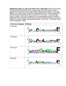
Supplementary Figure 3. Conserved domains among class III heme-peroxidases. Amino acid sequence alignment of POX12 with selected members of secreted ...
Shapiro-Wilk P= 0.597. Shapiro-Wilk P=0.685. Acetate.obs. Ethanol.obs. 0.04. 0.05. 0.00. O. O. O. Oo oo. O. -0.05. -0.04. TITI. -1.5 -0.5 0.5 1.5. Shapiro-Wilk P= ...
221. HAALSS. --CDP S. SVNV SEL HHTASPS-S. hTRNâSR1. 223 K A. DK-- N ... A HL. S D QR к ÑÑн. V. T E YD-. QYI R. SY P NEKQS VLPR-. â YQES KA SDI.
C. D. 1. 4. /1. 9. A le x a. -7. 0. 0. 0. 0. 50K. 100K. 150K. 200K. 250K. SSC-A. 85.5. 0. 10 3. 10 4. 10 5. C. D. 3. A. P. C. -H. 7. 0. 50K. 100K. 150K. 200K. 250K.
FIGURE S3 perinuclear region lamellar region. (μ m. 2. ) 10-3. 10-2. 10-1. 100. 10-3. 10-2. 10-1. 100. Time Lag, Ï (s). 10-1. 100. 101.
3. U. S-2. 4. U. S-2. 5. U. S-2. 6. Figure S3. SNP position. (in kb). 18 010. A G G G G G G G G G G G G G G G G G G G G G G G G G G G G G G G G G G A ...
PB S D. FIGURE S3. DEX/PBS DEX/rIL-21. rIL-Zl. W. N in. ETP n=3/gr0up m 2 0 .DN2 P< 0.05 a). $3â 1.5 i u. 2 1.0. 51. 0.5. 0. D 70 n=3/gr0up E 70 UDN3 n=3/ ...
Figure S3. Viral and target gene siRNAs in CaLCuV::Chl virus-infected wild type (Col-0) plants. (A) The 1961 bp ChlI-2 genomic locus is shown schematically ...
Page 1. S3 Figure. Lymphocytes. 42.6. FSC-A. S. S. C-A. Single Cells. 98.9. FSC-A. F. S. C-H. CD4+. 56.0. CD8+. 28.5. CD4 BV510. CD8 P. erCP. -Cy5.5.
3. 4 x 10. 5. 1 2 3 4. 0. 5. 10. 15. 20 x 10. 4. 1 2 3 4. â2. 0. 2 x 10. 5. Figure S3. Bar plot of Raw data (value=height of Late stage - height ofearly stage)_47peaks.
Figure S3: Analysis of proteasome composition in naive and listeria- infected WT mice. Organ lysates of liver (A) and spleen (B) of naïve and infected WT mice.
Figure S3. (A). (B). 0. 0.1. 0.9. 1. E1 tot. MAPK activity x a x b. 0. 5. 10. 15. 0. 0.2. 0.4 n. H. Density. P(n. H. >1)=0.9996. P(n. H. >2)=0.7421. P(n. H. >3)=0.5036.
Figure S3 (A)
(B)
1 0.9 Density
MAPK activity
0.4
0.1 0
xa
5
10
15
n
(D)
0.1 0
H
y2 0.1 0
2
2
1
0.5 (x −x )/(x −x ) 2
1
b
1 0 0
1
a
0.5 y −y 2
(G)
1
1
(H)
6
3
4
2
SN Density
1 0.9 y1
3
0 0
xa x1 xmx2xb E1tot
(F)
3
Density
y1
H
(E)
Density
1 0.9 y2
Density
MAPK activity
0 0
H
(C)
MAPK activity
0.2
xb
E1tot
P(n >1)=0.9996 H P(n >2)=0.7421 H P(n >3)=0.5036 H P(nH>4)=0.3196
2
1
SN xa x1x2 xb E1tot
0
0
0.5 (x −x )/|x −x | 2
1
b
a
1
0 0
0.5 y −y 1
1
2
(A), (C) and (F) Schematic plots defining variables useful in the discussion of the adjacent histograms. (B) Histogram of Hill coefficients (nH ≡ log(81)/ log(xb /xa )) for “Single-valued” bifurcation diagrams; xa and xb are inputs (E1tot ) that correspond to 10% and 90% maximum output (MAPK activity). The quantities xa and xb are similarly defined in (C) and (F). (D) and(E) Histograms for “Oscillatory” bifurcation diagram properties. The quantities x1 and x2 in (D) and (E) are defined in (C) as input concentrations at the Hopf bifurcation points. The quantity xm is defined as xm ≡ (x1 + x2 )/2 . The quantities y1 and y2 are the minimum and maximum MAPK activity along the oscillatory solution evaluated at xm . The red bar in (E) represents the bifurcation diagrams with y2 − y1 > 1 . (G) and (H) Histograms for “Hysteretic” bifurcation diagrams properties. The quantities x1 and x2 in (G) and (H) are defined in (F) as input concentrations at the Saddle-Node bifurcation points. The red bar in (G) represents bifurcation diagrams that are discarded while computing the distributions. The quantities y1 and y2 are defined as the MAPK activities at the corresponding Saddle-Node bifurcation points.