Finding NECTARs from Evolutionary Trees [Technical Report] Ling Chen1 2
Sourav S. Bhowmick2
1 L3S, University of Hannover, Germany School of Computer Engineering, Nanyang Technological University, Singapore
[email protected],
[email protected]
Abstract. Mining trees is very useful in domains like bioinformatics, web mining, mining semi-structured data, and so on. These efforts largely assumed that the trees are static. However, in many real applications, tree data are evolutionary in nature. In this paper, we focus on mining evolution patterns from historical tree-structured data. Specifically, we propose a novel approach to discover negatively correlated subtree patterns (NECTARs) from a sequence of historical versions of unordered trees.The objective is to extract subtrees that are negatively correlated in undergoing structural changes. We propose an algorithm called NECTAR-Miner based on a set of evolution metrics to extract NECTARs. NECTAR s can be useful in several applications such as maintaining mirrors of a website, maintaining XML path selectivity estimation, web advertisement placement strategy, and semantic XML search engine. Extensive experiments show that the proposed algorithm has good performance and can discover NECTARs accurately.
1
Introduction
Mining tree-structured data has gained tremendous interest in recent times due to the widespread occurrence of tree patterns in applications like bioinformatics, web mining, semi-structured data mining, and so on. Existing works on mining tree-structured data can be broadly classified into three categories: association rule mining [4], frequent substructure mining [3, 19], and classification/clustering [13, 20]. While these tree pattern mining techniques have been innovative and powerful, our initial investigation revealed that majority of the existing approaches of tree mining focus only on snapshot data, while in real life tree-structured data is dynamic in nature. For example, consider a sequence of tree-structured data in Figure 1. The black and gray circles represent the newly inserted nodes and deleted nodes, respectively. Typically, there are two types of changes to tree-structured data: changes to data content (e.g., leaf nodes in an XML tree) and changes to the structure of tree data (internal nodes). In this paper, we focus on the structural evolution of tree-structured data only. The evolutionary nature of structure of trees leads to two challenging problems in the context of data mining. The first one is to maintain the previously discovered knowledge. For instance, in frequent substructure mining, as the data source changes new frequent structures may emerge and some existing ones may not be frequent anymore. The second one is to discover novel knowledge by analyzing the evolutionary characteristics of historical tree data. Such knowledge is difficult or even impossible to discover from snapshot data efficiently due to the absence of evolution-related information. In this paper, we focus on the second issue. That is, we present techniques to discover a specific type of novel knowledge by mining the evolutionary features of tree-structured data.
S t1
St2
a b
c
d
e
g
i
l
k
m
St3
a b
g
e
o
h
j
i
l
n
j
k
b
d
h
S t4
a
g i
a
d
e
o
h
l
n
j
p
b
d r
e i
h
l p
j q
Fig. 1. Sequence of historical tree versions.
Let us elaborate informally on the types of novel knowledge one may discover by analyzing evolutionary features of trees. Consider the different versions of a tree structure in Figure 1. We may discover the following types of novel knowledge by exploiting the evolution-related information associated with the trees. Note that this list is by no means exhaustive. – Frequently Changing Structures (FCS): Different parts of a tree may evolve in different ways over time. Some parts of the tree may evolve more frequently than other parts. Some parts may change more significantly in the history compared to other parts that may only change slightly. For example, the subtree rooted at node b changes in all the four versions. On the other hand, the subtree rooted at d never changes. We refer to structures that change frequently and significantly in the history as frequently changing structures. Here, frequently refers to the large number of times the corresponding parts changed, while significantly refers to the large percentage of nodes that have changed in the corresponding subtree. – Associative Evolutionary Structures (AES): Similar to the transactional association rule, different parts of the tree may be associated in terms of their evolutionary features over time. For example, in Figure 1 one may observe that whenever subtrees rooted at i and ` change frequently and significantly, the subtree rooted at h does not change. Then, a negative association rule may be extracted between the subtrees with respect to some appropriately specified thresholds. Note that a positive association rule can similarly be discovered by discovering subtrees that change frequently and significantly together. We refer to such structures as associative evolutionary structures. We have discussed frequently changing structures in [21]. Hence, in this paper, we focus on discovering a specific type of associative evolutionary structures from historical treestructured data. Particularly, we propose a technique to discover subtrees that are negatively correlated in undergoing structural changes. That is, when a set of subtrees changes (significantly), another set of subtrees rarely changes (significantly). We refer to this type of patterns as NECTARs (NEgatively Correlated subTree pAtteRn). While this pattern can represent subtrees which may or may not be structurally related, in this paper, we focus on discovering NEC TAR s from subtrees having ancestor-descendant relationships. As we shall see in Section 5, NECTARs are useful in applications such as maintaining mirrors of Web site [10], maintaining XML path selectivity estimation, web advertisement placement, and semantic XML search engine [12]. Given a sequence of versions of a tree structure, we propose a set of evolution metrics to quantitatively measure the frequency and correlation of significant changes to subtrees. Based
on such metrics, we propose an algorithm called NECTAR-Miner to extract the NECTARs from the tree sequence. Our proposed algorithm consists of two major phases: the GDT construction phase and the NECTARs discovery phase. In the first phase, given a sequence of historical tree-structured data, the GDT (General Delta Tree) is constructed to efficiently represent evolutionary features of trees. The goal of second phase is to extract the negatively correlated subtrees by traversing the GDT. Our experimental results show that the proposed algorithm can successfully extract all the NECTARs efficiently. The rest of the paper is organized as follows. We begin by modeling structural changes to evolutionary tree data in Section 2. Next, in Section 3, we propose a set of metrics to quantitatively measure the evolutionary features of tree data and use these evolution metrics to formally define the notion of NECTARs. Section 4 describes the algorithm for mining NEC TAR s. We highlight the practical usefulness of NECTARs by discussing some applications in variety of domain in Section 5. We evaluate the performance of the NECTAR mining algorithm in Section 6. We review related work in Section 7. The last section concludes this paper.
2
Modeling Structural Changes to Trees
We first present different types of structural changes to tree-structured data and how we quantify the degree of change in the data. Next, we introduce the notion of structural delta which will be used subsequently in our discussion. We use the following notations in the sequel. Let S = hN, E, Li denotes a tree structure, T = ht1 , t2 , . . . , tn i be a sequence of time points with some particular time granularity, S ti be the version of S at time point ti , and si be a subtree of S, denoted as si ≺ S. 2.1 Types of Structural Changes An edit operation is an operation e that can be applied on a tree S1 = hN1 , E1 , L1 i to produce e another tree S2 = hN2 , E2 , L2 i, denoted as S1 → S2 . Given two versions of a tree structure, different types of edit operations have been defined in traditional change detection algorithms [8]. For instance, atomic edit operations such as insertion, deletion, and update can be defined based on nodes. Furthermore, complex operations on subtrees such as move, copy, and delete a subtree, can be defined as well. Usually, an edit operation defined on a subtree can be decomposed into a sequence of atomic edit operations defined on nodes. In our study, we consider the atomic edit operations defined on leaf nodes that cause structural changes to an unordered tree. Note that our work can easily be extended to ordered trees as well. Hence we define only two edit operations as follows: (a) INS(x(name), p): This operation creates a new leaf node x, with node label “name”, as a child node of node p in a tree. (b) DEL(x): This operation is the inverse of the insertion one. It removes leaf node x from a tree. For example, consider the first two tree versions, S t1 and S t2 , in Figure 1. The version t2 S can be produced from S t1 by applying the following structural edit operations: inserting nodes labeled n and o as a child of nodes e and b, respectively, and deleting nodes labeled c and m. Note that we do not consider the update operation because it does not incur structural changes. Certainly, depending on application the update operation can be regarded as deleting a node and inserting a node with a new label. Given two versions of a tree (subtree), edit distance is usually adopted in traditional change detection algorithms to measure the distance between the two versions. Edit distance is defined
based on edit script, which is a sequence of edit operations that converts one tree into another. Note that, in traditional change detection algorithms there may exist more than one valid edit script since the edit operations are decomposable. However, since we consider atomic structural edit operations, there exists only one valid edit script. Then, edit distance can be defined as follows. Given two versions of a trees S at time points tj and tj+1 , denoted as S tj and S tj+1 , let E(S tj → S tj+1 ) be a sequence of atomic edit operations, he1 , e2 , . . . , en i, which converts S tj to S tj+1 , then, the edit distance between the two versions, denoted as d(S tj , S tj+1 ), is the number of edit operations in the edit script. That is, d(S tj , S tj+1 ) = |E|. For instance, let the subtree a/b/e in Figure 1 be s. The following sequence of edit operations convert st1 to st2 : E(st1 → st2 ) = hDEL(m), IN S(n, e)i. Then, the edit distance between st1 and st2 , d(st1 , st2 ), is 2. 2.2
Degree of Changes
Considering that an edit distance is an absolute value which measures the difference between two tree structures, we define the Degree of Change (DoC) of a tree in two versions by normalizing the edit distance by the size of the consolidate tree of the two tree versions. Given two tree versions S tj = hN tj , E tj , Ltj i and S tj+1 = hN tj+1 , E tj+1 , Ltj+1 i, the consolidate tree of them, denoted as S tj ]S tj+1 , is hN, E, Li, where i) N = N tj ∪N tj+1 , ii) e = (x, y) ∈ E, if and only if x is the parent of y in E tj or E tj+1 . For example, the consolidate tree of a/b/e in the first two versions in Figure 1 contains the nodes e, i, k, `, m, and n. Definition 1 (Degree of Change). Given two versions of a tree S tj and S tj+1 , let d(S tj , S tj+1 ) be the edit distance between the two versions, then the Degree of Change of S from tj to tj+1 , denoted as DoC(S, tj , tj+1 ), is: DoC(S, tj , tj+1 ) = size of the consolidate tree of S tj and S tj+1 .
d(S tj ,S tj+1 ) |S tj ]S tj+1 |
where |S tj ] S tj+1 | is the
The value of DoC ranges from 0 to 1. If a tree does not change in two versions, then its DoC is zero. If a tree is totally removed or newly inserted, then the DoC of the tree is one. The greater the value of DoC, the more significantly the tree changed. For example, let the subtree a/b in Figure 1 be subtree s1 . Then the DoC of s1 in the first two versions is DoC(s1 , t1 , t2 ) = 4/12 = 0.33. 2.3 Structural Delta When a tree evolves from one version to another version, some of its subtrees change (i.e., their DoC values are greater than zero), while some of its subtrees remain unchanged (i.e., their DoC values equal to zero). We are interested in the set of changed subtrees. Particularly, we refer to the set of changed subtrees in two successive versions as the structural delta. Definition 2 (Structural Delta). Given two versions of a tree S at time tj and tj+1 , the structural delta of S from tj to tj+1 , denoted as ∆S (tj , tj+1 ), refers to the set of changed subtrees in the two versions and ∆S (tj , tj+1 ) = {s|s ≺ S tj & DoC(s, tj , tj+1 ) > 0} ∪ {s|s ≺ S tj+1 & DoC(s, tj , tj+1 ) > 0}. For example, consider the first two tree versions in Figure 1. ∆S (t1 , t2 ) = {a/b, a/b/c, a/b/e, a/b/e/l, a/b/e/l/m, a/b/e/n, a/b/o}. Note that the subscript S can be omitted if it is clear from the context.
3 Evolution Metrics We now introduce the metrics defined to measure the change frequency and change significance for a set of subtrees. Particularly, we use the following notations for the subsequent definitions. Let Σ = hS t1 , S t2 , . . . , S tn i be a sequence of versions of tree S on T , h∆(t1 , t2 ), . . . , ∆(tn−1 , tn )i be the sequence of corresponding structural deltas, Ω = ∆(t1 , t2 )∪ . . . ∪ ∆(tn−1 , tn ) be the set of all changed subtrees. 3.1 Frequency of Significant Change (FoSC) Note that DoC of a subtree measures how significantly a subtree changed in two successive versions. In order to justify whether a set of subtrees are correlated in undergoing significant changes, we need a metric to measure how frequently the set of subtrees undergoes significant changes together. Hence, we introduce the metric Frequency of Significant Change (F oSC) for a set of subtrees. Note that the metric F oSC is defined with respect to a given threshold of DoC because we say a subtree undergoes significant changes only if its DoC value is no less than the DoC threshold. Definition 3 (Frequency of Significant Change (FoSC)). Let X = {s1 , s2 , . . . , sm } be a set of changed subtrees, X ⊆ Ω, and the threshold of DoC be α. The Frequency of Significant P Change for the set X, with respect to α, denoted as F oSCα (X), is: F oSCα (X) = Qm where Dj = i=1 Dji and ½ 1, if DoC(si , tj , tj+1 ) ≥ α Dji = 1≤i≤m 0, otherwise
n−1 j=1 Dj (n−1)
That is, F oSCα of a set of subtrees is the fraction of subsequent versions (after the first version) where the set of subtrees undergoes significant changes together. The value of F oSCα ranges in [0, 1]. If all subtrees in the set undergo significant changes together in each subsequent version, then the value of F oSCα equals to one. If subtrees in the set never undergo significant changes together in subsequent versions, then the value of F oSCα is zero. For example, reconsider the sequence of historical tree versions in Figure 1. Let X = {a/b, a/b/e} and the threshold of DoC α be 1/4. Then, F oSC1/4 (X) = 2/3 as both subtrees undergo significant changes in two subsequent versions S t2 and S t4 . Let Y = {a/b/e, a/b/e/i}. Then F oSC1/4 (Y ) = 1/3 as the two subtrees undergo significant changes together only in the version S t3 . 3.2 Correlation of Change (CoC) We now define the metric to measure the correlation between subtrees in undergoing significant changes. Given a DoC threshold α, in each transition between two successive versions, a set of subtrees either undergoes significant changes together or not. This could be considered as a binary variable. Furthermore, it is a symmetric binary variable because we are interested in both the occurrences and the nonoccurrences of significant changes to subtrees. Hence, correlation measures which are suitable for analyzing symmetric binary variables can be used, such as φ-coefficient, odds ratio, and the Kappa statistic etc. [14]. In our analysis, we use the
Y
¬Y
a
∑row
b
a
b
a d
b
X
f11
f10
f1+
¬X
f01
f00
f0+
∑col
f+1
f+0
M
c
e
i
g n
l m
k
o
p
q
c
r i
l
k
m
(b) general delta tree
(a) 2X2 contingency table
e
g
o
n
h j
c
o e l
n
m (c) result tree
(d) delta tree
Fig. 2. 2 × 2 contingency table, general delta tree and delta tree.
φ-coefficient. Given the contingency table in Figure 2(a), where X (Y ) represents that a set of subtrees X (Y ) undergoes significant changes together and ¬X (¬Y ) represents subtrees in X (Y ) do not undergo significant changes together, the φ-coefficient between variables X and Y can be computed by the following equation. M f11 − f1+ f+1
φ(X, Y ) = p
f1+ (M − f1+ )f+1 (M − f+1 )
(1)
Particularly, in our mining context, the value of M in Figure 2(a) equals to n − 1, which is the total number of transitions between successive historical versions. Furthermore, f11 refers to the number of versions where all subtrees in X and Y undergo significant changes together. Hence, f11 equals to F oSCα (X ∪Y )×(n−1). Similarly, f1+ equals to F oSCα (X)×(n−1) and f+1 equals to F oSCα (Y ) × (n − 1). Thus, the Equation 1 can be transformed as the following one, which is formally defined as Correlation of Change (CoC). Definition 4 (Correlation of Change (CoC)). Let X and Y be two sets of subtrees, s.t. X ⊆ Ω, Y ⊆ Ω, and X ∩ Y = ∅. Given a DoC threshold α, the Correlation of Change of X and Y , with respect to α, denoted as CoCα (X, Y ), is: F oSCα (X ∪ Y ) − F oSCα (X) ∗ F oSCα (Y )
CoCα (X, Y ) = p
F oSCα (X)(1 − F oSCα (X))F oSCα (Y )(1 − F oSCα (Y ))
According to the definition of φ-coefficient, if CoCα (X, Y ) is greater than zero, two sets of subtrees X and Y are positively correlated in undergoing significant changes. Otherwise, they are negatively correlated in undergoing significant changes. In the following discussion, the subscript α in both F oSCα and CoCα is omitted if α is understood in the context. For example, consider the sequence of historical versions of tree S in Figure 1 again. Let the threshold of DoC α be 1/3. Let X = {a/b, a/b/e} and Y = {a/b/e/i}. CoC1/3 (X, Y ) = √ 3×0−2×1 = −1. Hence, {a/b, a/b/e} and {a/b/e/i} are negatively correlated in 2×(3−2)×1×(3−1)
undergoing significant changes. 3.3
NECTAR
Mining Problem
Based on the evolution metrics introduced above, various negatively correlated subtree patterns or NECTARs can be defined. For example, we can define the pattern as two sets of subtrees with a negative CoC value. The subtrees may or may not be structurally independent.
Particularly, in this paper, we define NECTAR on subtrees with ancestor-descendant relationships. Let si be an ancestor subtree of si+1 (conversely, si+1 be a descendant subtree of si ), denoted as si  si+1 , if there is a path from the root of si to the root of si+1 . Then, NECTARs can be defined as follows. Definition 5 (NECTARs). Given the DoC threshold α, the F oSC threshold η, and the CoC threshold ζ (0 ≤ α, η ≤ 1, ζ ≥ 0), P = hX, Y i, where X = hs1 , s2 , . . . , sm−1 i, Y = hsm i, and si  si+1 (1 ≤ i < m), is a NECTAR if it satisfies the following conditions: (i) F oSCα (X) ≥ η; (ii) F oSCα (P ) < η; (iii) CoCα (X, Y ) ≤ −ζ. Consider the sequence of historical versions of tree S in Figure 1 again. Suppose the threshold α = 1/3, η = 2/3, and ζ = 1/2. hha/b, a/b/ei, ha/b/e/iii is a NECTAR because F oSC({a/b, a/b/e}) = 2/3 ≥ η, while, F oSC ({a/b, a/b/e, a/b/e/i}) = 0 < η and CoC ({a/b, a/b/e}, {a/b/e/i}) = −1 < −ζ. Such a pattern indicates that subtrees a/b and a/b/e frequently undergo significant changes together. Whereas, when the two subtrees change significantly, the subtree a/b/i rarely change significantly. A NECTAR hhs1 , s2 , . . . , sm−1 i, hsm ii indicates that the sequence of subtrees hs1 , s2 , . . . , sm−1 i frequently undergo significant change together. Whereas, they rarely undergo significant changes together with a descendant subtree sm . Based on the inferred knowledge, we identified two types of subsumption relationships between NECTARs as follows. Definition 6. (Tail Subsumption) Given two NECTARs P1 = hX, Y1 i and P2 = hX, Y2 i, where Y1 = hsx i and Y2 = hsy i, we say P1 tail-subsumes P2 (or P2 is tail-subsumed by P1 ), denoted as P1 At P2 , if sx  sy . Definition 7. (Head Subsumption) Given a NECTARs P1 = hX1 , Y1 i and a subtree sequence X2 s.t. F oSC(X2 ) ≥ η, where X1 = hs1 s2 · · · sm i and X2 = hv1 v2 · · · vn i, we say P1 is head-subsumed by X2 , denoted as P1 @h X2 , if ∃i(1 < i ≤ m ≤ n) such that s1 = v1 , · · · , si−1 = vi−1 , and si ≺ vi . Consider example in Figure 1 again. If both hha/bi, ha/b/eii and hha/bi, ha/b/e/iii are then the former tail-subsumes the latter. If the subtree sequence S = ha/b, a/b/ei satisfies the FoSC threshold, then all NECTARs hha/b, a/b/e/ii, Y i are head-subsumed by the sequence S, where Y can be any descendant subtree of a/b/e/i. Often we observe that subsumed NECTARs add no further value to applications of NEC TAR s [10]. Hence, we exclude the subsumed NECTARs from the task of NECTAR mining. Thus, the problem of NECTAR mining can be formally defined as follows. NECTARs,
Definition 8 (NECTAR Mining). Given a sequence of historical versions of a tree structure, the DoC threshold α, the F oSC threshold η and the CoC threshold ζ, the problem of NEC TAR mining is to find the complete set of NECTARs where each satisfies the specified thresholds and is neither tail-subsumed or head-subsumed.
4
NECTAR - MINER
Algorithm
Given a sequence of historical versions of a tree structure and thresholds of DoC and F oSC, the general algorithm NECTAR Miner is shown in Figure 3(a). Note that, although it is optimized for nonsubsumed NECTARs, it can easily be extended to mine all NECTARs. Also, the
threshold of CoC does not need to be given manually. Cohen [11] discussed the strength of the φ-coefficient value. It is stated that the correlation is strong if |φ| is above 0.5, moderate if |φ| is around 0.3, and weak if |φ| is around 0.1. Based on this argument, the CoC threshold can be set automatically and progressively. In our algorithm, we set the initial threshold of CoC ζ as 0.5. If no NECTAR is discovered with respect to this value and ζ is greater than 0.3, ζ is decreased successively. With a given ζ, basically, there are two phases involved in the mining procedure: – Phase I: GDT Constructor. Given the input as a sequence of historical versions of a tree structure, the first phase has two subtasks. Firstly, structural deltas, which contain changed subtrees in each two successive versions, should be detected. Secondly, structural deltas should be organized into an appropriate data structure. Particularly, we propose a data structure, called General Delta Tree (GDT ), which not only records the changed subtrees but also preserves the ancestor-descendant relationships between subtrees. We discuss the details of this phase in the next subsection. – Phase II: NECTAR Discovery. The input of this phase is the GDT constructed in the previous phase. We mine NECTARs with respect to a set of thresholds of DoC, F oSC and CoC. NECTARs are discovered with the divide-and-conquer strategy. 4.1 Phase I: GDT Construction Given a sequence of historical versions of a tree structure, we construct a data structure, called General Delta Tree (GDT ), that is appropriate for NECTAR mining. A GDT not only registers change information of subtrees, such as their DoC values, but also preserves the structural information of subtrees, such as the ancestor-descendant relationships. Definition 9 (General Delta Tree). Given a sequence of historical tree versions Σ, a se0 quence of consolidate trees of each two successive versions can be obtained, hS1 = hN1 , E1 i, 0 0 0 S2 = hN2 , E2 i, · · · , Sn−1 = hNn−1 , En−1 ii, where Si = S ti ] S ti+1 . A General Delta Tree GDT = hN, Ei, where N = N1 ∪ N2 ∪ · · · ∪ Nn−1 and e = (x, y) ∈ E only if x is a parent of y in any Ei (1 ≤ i ≤ n − 1). Each node x is associated with a vector where the ith element t corresponds to DoC(stxi , sxi+1 ). Consider the sequence of historical tree versions in Figure 1. The constructed general delta tree is shown in Figure 2(b). Note that for clarity, we show the vector of DoC values for some of the nodes only. The node b is associated with a sequence h1/3, 2/11, 5/11i, which indicates that the DoC value of the subtree a/b in the first two versions is 1/3, DoC(a/b, t2 , t3 ) = 2/11, and DoC(a/b, t3 , t4 ) = 5/11. The algorithm of this phase is shown in Figure 3(b). At first, we initialize the root node of GDT . Then, for each two successive tree versions, we employ the algorithm X-Diff [16] to detect changes to tree structures1 . We adapt the algorithm slightly so that it directly takes generic tree structures as input. Given two tree versions, X-Diff generates a result tree which combines the nodes in both versions. For example, Figure 2(b) shows the example result tree generated by X-Diff after detecting changes between the first two tree versions in Figure 1. Here, we use gray nodes to represent the deleted nodes and black nodes to represent the inserted nodes. 1
Note that our technique is not dependent on a specific tree differencing algorithm. Hence, it can work with any tree-diff approach.
Input: Σ= Output: a general delta tree GDT Description: 1: initialize GDT 2: for ( i = 0; i < n; i++ ) do 3: result_treei = X-Diff’ (Sti, Sti+1); 4: initialize delta_treei.root with result_treei.root 5: for each child x of result_treei.root 6: Depth_Traverse(x, delta_treei.root ) 7: end for 8: delta_treei.root.descendants += x.descendants 9: delta_treei.root.changed_descendants += x.changed_descendants 10: Merge_Tree(GDT.root, delta_treei.root, i) 11: end for 12: return GDT
Input: Σ=, α, η Output: a set of NECTARs Ρ Description: ζ = 0.5 1: 2: GDT = GDT_Constructor(Σ) 3: while((| Ρ | == 0)&&(ζ > 0.3)) 4: Ρ = Ρ ∪ Total_Pattern_Miner (GDT.root, α, η, ζ) ζ -5: 6: return Ρ
(a) Algorithm: NECTAR_Miner
(b) Algorithm: GDT_Constructor
Input: x, α, η, ζ Output: total set of NECTARs P Description: 1: if(FoSCα (sx) ≥ η) then 2: P = 3: P.bitmap = Trans2Bit(x.DoCs, α) 4: P = P ∪ Part_Pattern_Miner (x, P, α, η, ζ) 5: end if 6: for(each child y of x ) do 7: Total_Pattern_Miner(y, α, η, ζ) 8: end for 9: return P
Input: x, x’, i Description: 1: the ith element of x.DoCs = x’.changed_descendants/x’.descendants 2: for ( each child y’ of x’) do 3: if (x has no matching child y) then 4: create a child y of x corresponding to y’ 5: end if 6: Merge_Tree(y, y’, i) 7: end for
(c) Algorithm: Total_Pattern_Miner
Input: nodes x, y Description: 1: Create a child x’ of y corresponding to x 2: x’.descendants = 1 3: if(x is inserted/deleted) then 4: x’.changed_descendants = 1 5: end if 6: for( each child z of x ) 7: Depth_Traverse(z, x’ ) 8: x’.descendants += z.descendants 9: x’.changed_descendants += z.changed_descendants 10: end for 11: if (x’.changed_descendants == 0) then 12: remove x’ from delta_tree 13: end if
(e) Algorithm: Depth_Traverse
(d) Algorithm: Merge_Tree Input: x, P, α, η, ζ Output: NECTARs starting from sx: Px Description: 1: for (each child y of x) do 2: if(FoSCα (P∪ sy) ≥ η) 3: then 4: P = P∪ < sy > 5: P.bitmap = P.bitmap ∩ Trans2Bit(y.DoCs, α) 6: Px = Px ∪ Part_Pattern_Miner (y, P, α, η, ζ) 7: else 8: if(CoCα(P, ) ≤ - ζ ) then 9: Px = Px ∪ P 10: end if 11: end if 12: end for 13: return Px (f) Algorithm: Part_Pattern_Miner
Fig. 3. NECTAR-miner algorithm.
For each result tree generated by X-Diff, we employ the algorithm Depth Traverse to generate a delta tree which contains change information of subtrees. The Depth Traverse algorithm is shown in Figure 3(e). Basically, Depth Traverse traverses the result tree in the depth-first order. While reaching a node x in the result tree, we create a corresponding node in the delta tree and maintain two counters for the node: descendants and changed descendants. The former records the number of descendants of x while the latter records the number of inserted/deleted descendants of x. Then, the DoC value of the subtree rooted at x can be computed by dividing changed descendants by descendants. If the DoC value equals to zero, we remove the node from the delta tree because the subtree rooted at x is not a changed subtree. Otherwise, we associate the DoC value with the node. For example, after performing Depth Traverse on the result tree in Figure 2(c), the generated delta tree is shown in Figure 2(d).
Then, for each generated delta tree, we merge it into the GDT. The algorithm is shown 0 in Figure 3(d). When merging the ith delta tree (subtree) rooted at node x with the GDT (subtree) rooted at node x, we only need to set the ith element of the DoC sequence of x with the DoC value of sx0 . Then, the algorithm iteratively merges their children with the same 0 0 label. For a child y of x , if x does not have any matching child, we create a child node of x labeled as y. We associate a DoC sequence with the new child node such that the ith element 0 of the sequence is set as the DoC value of y . Let |S| be the maximum size of the historical tree versions and |∆S| be the maximum size of the result trees. Then, the complexity of the first phase can be computed as follows. The initialization of GDT is O(|∆S|). The complexity of generating a delta tree is O(|S|2 × deg(S) × log2 (deg(S))), where deg(S) is the average out-degree of nodes in tree versions [16]. For each result tree, we traverse it to calculate the DoC for each node and then merge it to the GDT if its DoC is greater than zero. Thus, the complexity of this operation is O(2|∆S|). Hence, the dominant cost is the change detection step, which is iterated n − 1 times. Hence, the complexity of phase I is O((n − 1) × (|S|2 × deg(S) × log2 (deg(S)))). 4.2 Phase II: NECTAR Discovery The input of this phase is the GDT and the thresholds α, η and ζ of DoC, F oSC and CoC. We aim to discover all non-subsumed NECTARs satisfying the thresholds from the GDT . The complete set of NECTARs P can be divided into disjoint partitions, P = P1 ∪ P2 ∪ . . . ∪ Pm , such that each partition contains NECTARs starting from the same subtree. That is, ∀Px = hhsx sx+1 . . . sx+m i, hsx+m+1 ii ∈ P, Py = hhsy sy+1 . . . sy+n i, hsy+n+1 ii ∈ P, if sx = sy then Px , Py ∈ Pi ; otherwise, Px ∈ Pi , Py ∈ Pj (i 6= j, 1 ≤ i, j ≤ m). Therefore, the discovery of the complete set of NECTARs can be divided into subproblems of mining patterns for each partition, where each pattern begins with the same subtree. The algorithm of the second phase is shown in Figure 3(c). We mine patterns by traversing the GDT with the depth-first order. For each node x, which represents the subtree sx , if the value of F oSC(sx ) is no less than the threshold η, we call the function P art P attern M iner to discover NECTARs starting from sx . Note that, the F oSC(sx ) can be computed with the vector of DoC values associated with node x. For example, consider the GDT in Figure 2(a). Let α = 0.3 and η = 0.3. The vector of DoC values of node b is h2/5, 2/11, 5/11i ≈ h0.40, 0.18, 0.45i. Then, F oSC(a/b) = 2/3 ≈ 0.67 > η. Thus, we need to find NECTARs starting from subtree a/b. Before mining NECTARs starting from some subtree sx , we initialize a pattern P = hsx i and associate a bitmap with the pattern. In a bitmap, there is one bit for each element of the DoC sequence of node x. If the ith element is greater than α, then bit i is set to one. Otherwise, bit i is set to zero. For example, before mining NECTARs starting from a/b in the GDT in Figure 2(a), the bitmap associated with P = ha/bi is h101i if α is set as 0.3. The algorithm Part Pattern Miner is shown in Figure 3(f ). For a particular node x in GDT , it generates all non-subsumed NECTARs starting from sx . Note that, we directly mine non-subsumed NECTARs instead of performing filtering process afterwards. For this purpose, we employed the following three strategies in Part Pattern Miner. Firstly, when mining NEC TAR s starting from a subtree sx , candidate patterns are generated and examined by traversing sx with the depth-first manner. As shown in Figure 3(f ), Part Pattern Miner performs a depth-first traversal on the subtree rooted at node x. This strategy facilitates the performing of
the following two strategies. Secondly, once a sequence of subtrees satisfying the FoSC threshold is discovered, candidate patterns must be extended from this sequence. For example, as shown in the Lines 4 to 6 of Part Pattern Miner, given the subtree rooted at node x and current pattern hsx i, for each child y of x, if F oSC({sx , sy }) satisfies the threshold η, the pattern is updated as P = hsx , sy i. Simultaneously, the bitmap of P is also updated with the DoC vector of node y. Then, Part Pattern Miner is recursively called for the updated pattern. This strategy prevents generating NECTARs which are head-subsumed. Thirdly, once a NECTAR is discovered, we stop traversing nodes deeper than the current one. For example, as shown in Lines 8 and 9 of Part Pattern Miner, if CoC({sx }, {sy }) < −ζ, a NECTAR hhsx i, hsy ii is discovered. Part Pattern Miner is not recursively called any more. This strategy keeps from generating NECTARs that are tail-subsumed. For example, consider the GDT in Figure 2(a) again. Let the thresholds α = 0.3, η = 0.3 and ζ = 0.5. P art P attern M iner mines NECTARs starting from subtree a/b as follows. The initial pattern P = ha/bi and its bitmap is h101i. For the child node e of b, since DoC vector of e is h1/3, 1/3, 1/3i ≈ h0.33, 0.33, 0.33i, then F oSC({a/b, a/b/e}) = 2/3 > η. Hence, the pattern is updated as P = ha/b, a/b/ei and its updated bitmap is h101i. Then, we further find NECTARs starting from ha/b, a/b/ei. For the child node i of e, since F oSC({a/b, a/b/e, a/b/e/i}) = 0 < η and CoC0.3 ({a/b, a/b/e}, {a/b/e/i}) = −1 < −ζ, then hha/b, a/b/ei, ha/b/e/iii is discovered as a NECTAR. For the child node l of e, since F oSC({a/b, a/b/e, a/b/e/l}) = 1/3 > η, the pattern, together with its bitmap, is updated. Then, we further search NECTARs starting from ha/b, a/b/e, a/b/e/li and discover the NEC TAR s hha/b, a/b/e, a/b/e/li, ha/b/e/l/pii. The algorithm terminates when all descendants of node b are visited. Lemma 1. No subsumed NECTAR will be discovered NECTAR Miner. Proof: Suppose a NECTAR P1 = hhs1 s2 · · · sm−1 sm i, hsm+1 ii is head-subsumed by a subtree sequence X2 = hs1 s2 · · · sm−1 sn i with F oSC(X2 ) ≥ η. Since P1 @h X2 , sm ≺ sn . According the first strategy, X2 is examined earlier than hs1 s2 · · · sm i. And since F oSC(X2 ) ≥ η, according to the second strategy, candidate pattern will be extended from X2 . Hence, NECTARs starting with hs1 s2 · · · sm−1 sm i will not be generated. Otherwise, it contradicts to Strategy 2. That is, no head-subsumed NECTARs will be generated. Given a NECTAR P1 = hX, hsm ii, if there exists another NECTAR P2 = hX, hsm+1 ii s.t. P1 @t P2 , then sm ≺ sm+1 . Then, it contradicts with the third strategy. Hence, there is neither headsubsumed nor tail-subsumed NECTARs will be generated by NECTAR M iner. The complexity of the second phase can be computed as follows. We traverse each node in the GDT . For each interesting subtree rooted at node x, we call the P art P attern M iner method which needs to traverse each node in the subtree sx . Hence, each node in GDT is traversed at most m times, where m is the depth of the node. Then, let the depth of GDT be dep(GDT ), the complexity of this phase is O(|GDT | × dep(GDT )). Theorem 1. The algorithm NECTAR M iner discovers the set of non-subsumed NECTARs completely. The correctness of NECTAR M iner comes from the completeness of the GDT and the correctness of P art P attern M iner. Since GDT not only records each changed subtree and its DoC in each successive versions but also preserves the ancestor-descendant relationship between subtrees, all information in relevance to NECTAR mining is maintained. The three
Dynamic Summary
Estimator
(path table)
(Bloom histogram)
XML Data
Path /a /a/b /a/b/c ... /a/d
Count 10 500 5 ... 300
construction update
update (a) system overview
(b) path table
Fig. 4. Bloom histogram.
strategies employed by P art P attern M iner ensure that each potential pattern is either examined or skipped to avoid generate subsumed NECTARs. Hence, NECTAR M iner is complete in discovering non-subsumed NECTARs.
5
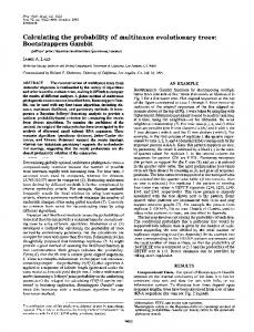
Representative Applications of NECTARs
Maintaining autonomous Web mirrors. A mirror site is a replica of an original Website and is often located in a different place throughout the Internet so that the original site can be accessed from more than one place. Web mirroring can be generally classified as internal mirroring and external mirroring. The former refers to the situation that both the original site and mirror sites are set up and maintained by the same organization. The latter means that the original site and mirror sites are autonomous. A mirror site should be updated frequently to ensure that it reflects the content of the original site. Although for internal mirroring this process can be performed efficiently by synchronizing mirror sites only if the original site evolves, for external mirroring the server holding the mirror site has to scan the original site frequently to detect the changes and update its local copy. Obviously, if the size of the Web site directory is large, such frequent scan and update may incur heavy workload. Hence, optimized mirror maintenance strategies are needed to improve the efficiency of external mirror maintenance. NECTARs can be mined from historical directory hierarchies of Web sites for more efficient mirror site maintenance [10]. When maintaining the mirror of a changed target directory, its subdirectories, which have positive evolution association with it, should not be skipped from mirroring since they frequently change significantly together. On the contrary, the mirror maintenance process can be optimized by skipping the subdirectories which have negative evolution association with it since these subdirectories rarely undergo significant changes together with the target directory. Discovered patterns are then used to design optimal strategies for autonomous Web mirror maintenance. Maintaining XML path selectivity estimation. Cost-based XML query optimization calls for accurate estimation of the selectivity of path expressions, which are commonly used in XML query languages to locate a subset of XML data. Recently, Bloom Histogram [17] has been proposed as a framework for XML path selectivity estimation in a dynamic context. There are three basic components in the system: the data file, the dynamic summary and the estimator (Figure 4). The data file refers to the XML file which is usually large. The dynamic summary keeps the necessary information of the data and the estimator is responsible for efficiently estimating the selectivity of path expression queries. The dynamic summary usually uses a
path table to record the frequency of occurrences of paths. When an XML file evolves, the system needs to rebuild the path table completely before updating the estimator. We can use NECTARs to selectively rebuild the path table rather than building it from scratch. Specifically, some paths in the path table do not need to be updated if their frequency of occurrences change insignificantly. For example, we can mine NECTARs from historical XML tree versions to discover when the support2 of some paths change significantly, the support of some path rarely undergoes significant changes together. Then, when updating the occurrence for a path, e.g., //a/b, whose support changes significantly, we check whether any child of node b forms a NECTAR with nodes on the path. Suppose a child c of b forms a NECTAR with a and b, we do not update the path //a/b/c in the path table as the support of the path may not change or change insignificantly. Intelligent web advertisement placement. It has been claimed that 99% of all web sites offer standard banner advertisements [6], underlying the importance of this form of on-line advertising. For many web-based organizations, revenue from advertisements is often the only or the major source of income (e.g., Yahoo.com, Google.com) [1]. One of the ways to maximize revenues for the party who owns the advertising space is to design intelligent techniques for the selection of an appropriate set of advertisements to display in appropriate web pages. Selection of banner advertisements is currently driven by the nature of the banner advertisement, Internet knowledge of the target market, relevance of the web page contents, and popularity of the web pages [1]. However, none of these techniques consider the evolution of web access patterns for the advertisement selection problem. As web access patterns can be modeled as unordered trees [15], NECTARs can be useful for designing more intelligent advertisement placement strategies. Intuitively, subtrees in a sequence of web access pattern trees that change together significantly represents different pages visited by users at different time points. Hence, it does not make sense to put relevant banner advertisements on these pages as they may not be visited in the future. On the other hand, subtrees that are negatively correlated and do not change significantly reflect stable collection of pages visited by web visitors over a period of time. Consequently, it makes sense to put relevant banner advertisements on these pages in order to maximize revenues. For example, suppose Figure 1 represents a sequence of web access sequences. Then using our strategy it make sense to put relevant advertisements in the subtree rooted at h as the remaining web access sequences in the subtree b are highly dynamic over time. Application to semantic search engines for XML: Recently, there has been research efforts for laying the foundations for semantic search engine over XML documents [12]. Given a set of keyword-label combinations as input, a semantic XML search engines typically returns semantically related fragments, ranked by estimated relevance. The underlying technique exploits the structural relationships of elements and does not exploit the evolutionary history of documents to extract semantic relationships to facilitate search. We believe that it is possible to predict semantic relationship between parts of documents by observing their evolutionary association among subtrees. For example, if we know that whenever a subtree s1 changes another subtree s2 do not change (NECTAR pattern) then it may indicate that the content of these two subtrees are not semantically related. Such knowledge can be used to filter search results as well as influence their estimated relevance. 2
The support of a path refers to the number of occurrences of the path in the document. The definition of DoC can be adjusted easily to measure the degree of support change.
Data Feature Parameters D1 V = 50, C = 3% D2 V = 50, C = 6%
F D
Fanout of the first tree version Depth of the first tree version
10 10
N V
Size of the first tree version Number of tree versions
1K 50
D3 D4
V = 50, C = 12% N = 1K, C = 3%
C
Change percent between tree versions
3%
D5
N = 1K, C = 6%
Data Feature Parameters D6 N = 1K, C = 12% D7 D8
N = 10K, V = 200, C = 3% N = 10K, V = 200, C = 6%
D9
N = 10K, V = 200, C = 12%
(b) Dataset List
(a) Parameter List
Fig. 5. Parameters and datasets.
6 Experimental Results The NECTAR mining algorithm is implemented in the Java programming language. All experiments are conducted on a Pentium IV 2.8GHz PC with 512 MB memory. The operating system is Windows 2000 professional. 6.1 Datasets We implemented a synthetic data generator which generates sequential tree versions. The set of parameters used by the generator are shown in Figure 5(a). At first, the generator constructs the first historical tree version, S t1 , based on parameters F , D and N . The first tree version is generated using the following recursive process. At a given node in the tree S t1 , we decide how many children to generate. The number of children is sampled uniformly at random from 0 to F . Before processing children nodes, we assign random probabilities to decide whether a child node is a leaf node, as long as tree depth is less than the maximum depth D. If a child node is not a leaf node and the total number of nodes is less than N , the process continues recursively. Once the first tree version has been created, we create as many subsequent versions as specified by the parameter V . The tree version S ti is generated based on the version S ti−1 with parameter C. For example, if the value of C is 3% and the number of nodes in the tree S ti is Ni , then the number of inserted and deleted nodes between trees S ti and S ti−1 is 3% × Ni . We randomly decide the positions of inserted and deleted nodes. Basically, there are 9 datasets used in the following experiments. The key parameter values used in generating the datasets are shown in Figure 5(b). 6.2 Scaleup Evaluation As analyzed before, the two dominant factors that affect the complexity of the algorithm are the average size of trees and the number of historical versions. Hence, we evaluate the scalability of the algorithm by varying the two parameters. We conduct the first experiment on the three data sets D1 , D2 and D3 . For each data set, we vary the size of the first tree version from 1K nodes to 16K nodes. The thresholds of DoC, F oSC and CoC are set as 0.001, 0.01, and 0.3, respectively. The experimental results are shown in Figure 6(a). It can be observed that the scale-up feature of the mining algorithm is basically linear to the size of trees. Furthermore, the smaller the change percent, the faster the mining algorithm. We conduct the second experiment on the three data sets D4 , D5 and D6 . For each data set, we vary the number of versions from 50 to 800. The thresholds of DoC, F oSC and CoC are
12% percent 4000
3000 1000
2000
4000
8000
16000
Execution Time (Sec)
Execution Time (ms)
3% percent 6% percent
5000
3%per cent 6%per cent 12%per cent
70 60 50 40 30 20 10 0 50
100
200
400
800
Number of Versions
Number of Nodes
(a) Variation on tree size
(b) Variation on version numbers
5
Phase I Phase II
4 3 2 1 0 1000
2000
4000
8000
16000
Execution Time (ms)
Execution Time (Sec)
Fig. 6. Experimental results I.
1500 1000 500 0 0.01
Number of Nodes
(a) Run time of phases
3%per cent 6%per cent 12%percent
2000
0.03
0.05
0.08
0.1
Threshold of DoC
(b) Variation on DoC Threshold
Fig. 7. Experimental results II.
set as 0.001, 0.01, and 0.3, respectively. The experimental results are shown in Figure 6(b). We observed that when the number of versions increases, the run time increases quickly because the sizes of subsequent trees increase as well. The respective scaleup feature of the two phases of the mining algorithm was studied as well on D4 with 50 versions. Figure 7(a) shows the results. Both phases take more time when the tree size increases. However, the first phase dominates the efficiency of the algorithm. 6.3 Efficiency Evaluation We now study how the thresholds of DoC, F oC, and CoC affect the efficiency of the algorithm. We show the run time of the second phase as the thresholds do not interfere the performance of the first phase. Experiments are conducted on the data sets D7 , D8 and D9 . The results of varying the threshold of DoC are shown in Figure 7(b). The F oSC threshold and CoC threshold are set as 0.01 and 0.3 respectively. It can be observed that the greater the DoC threshold value, the more efficient the algorithm. This is because when the DoC threshold value is greater, fewer subtrees are interesting enough so that we need to mine few negative evolution patterns. Figure 8(a) shows the results of the experiments on varying the threshold of F oSC. The thresholds of DoC and CoC are set as 0.001 and 0.3 respectively.
1200 1000 800 600 400 200 0 0.01
0.1
0.5
0.9
Execution Time (ms)
Execution Time (ms)
3%percent 6%percent 12%percent
3%percent 12%percent 1200 1000 800 600 400 200 0 0.3
0.4
0.5
0.6
Threshold of CoC
Threshold of FoSC (a) Variation on FoSC Threshold
6%percent
(b) Variation on CoC Threshold
Fig. 8. Experimental Results III.
We noticed that the greater the FoSC threshold, the more efficient the algorithm. Finally, Figure 8(b) shows that the variation on the CoC threshold has no affection on the performance of the mining algorithm, as illustrated by the complexity analysis.
7
Related Work
Although traditional association rule mining focuses on mining positive associations between items, it was observed that negative associations were useful as well in some situations [18]. Several work have been conducted on mining negative association rules [5][2][18]. They are different from each other in the employed correlation metrics. Consequently, the developed data mining algorithms are different as well. For example, Wu et al. [18] added on top of the support-confidence framework another measure called mininterest. They developed levelwise algorithms to find interesting itemset pairs first and then derive negative association rules. Antonie and Za¨ıane [2] used the correlation coefficient and integrated two phases to mine patterns and derive rules together. To the best of our knowledge, there exists no work on mining negative associations from changes to tree structure. Furthermore, our rules are distinguished in the way that the trees have ancestor-descendant relationships. Recently, the evolutionary feature of data was addressed by some data mining work which aim to maintain consistent mining results over time. For instance, Chakrabarti et al. [7] proposed to cluster timestamped data such that a clustering at each timestep is similar to the clustering at the previous timestep. Furthermore, each clustering should accurately reflect the data arrived during that timestep. Most of these approaches are different in the way that they cope with the dynamic nature of data by designing evolutionary approaches to update knowledge, whereas we mine the evolutionary tree data to obtain novel knowledge. In our previous work [9], we proposed a novel approach for mining structural evolution of XML data to discover FRACTURE patterns. A FRACTURE pattern is a set of subtrees that frequently change together and frequently undergo significant changes together. NECTARs are different from FRACTUREs in at least the following two aspects. First, since the former focus on the negative evolution associations while the latter capture the positive evolution associations, different evolution metrics are used. Second, the former are defined on a sequence of subtrees with ancestor-descendant relationships, while the latter are defined on subtrees which may or may not be structurally related.
8 Conclusions This work is motivated by the fact that existing tree mining strategies focus on discovering knowledge based on statistical measures obtained from the static characteristics of tree data. They do not consider the evolutionary features of the historical tree-structured data. In this paper, we proposed techniques to discover a novel type of pattern named negatively correlated subtree pattern (NECTAR) by analyzing the associations between structural evolution patterns of subtrees over time. NECTARs can be useful in several applications such as maintaining mirrors of a website, maintaining XML path selectivity estimation, web advertisement placement strategy, and semantic XML search engine. Two evolution metrics, F oSC and CoC, which measure the frequency and correlation of significant changes to historical tree-structured data, respectively, are defined to evaluate the interestingness of NECTARs. A data mining algorithm NECTAR-Miner based on divide-and-conquer strategy is proposed to discover NECTARs. Experimental results showed that the proposed algorithm has good performance and can accurately identify the NECTARs.
References 1. A. Amiri and S. Menon. Efficient scheduling of internet banner advertisements. ACM TOIT, 3(4):334–346, 2003. 2. M. Antonie and O. R. Zaiane. Mining Positive and Negative Association Rules: An Approach for Confined Rules. In PKDD, 2004. 3. T. Asai, K. Abe, S. Kawasoe, H. Arimura, H. Sakamoto, and S. Arikawa. Efficient Substructure Discovery from Large Semi-structured Data. In Proc. of SIAM DM, pp. 158–174, 2002. 4. D. Braga, A. Campi, S. Ceri, M. Klemettinen, and P. L. Lanzi. Mining Association Rules from XML Data. In Proc. of DAWAK, pp. 21–30, 2000. 5. S. Brin, R. Motwani, and C. Silverstein. Beyond Market Baskets: Generalizing Association Rules to Correlations. In SIGMOD, 1997. 6. C. Buchwalter, M. Ryan, and D. Martin. The state of online advertising: data covering 4th Q 2000. TR AdRelevance, 2001. 7. D. Chakrabarti, R. Kumar, and A. Tomkins. Evolutionary Clustering. In KDD, pages 554–560, 2006. 8. S. Chawathe and H. Garcia-Molina. Meaningful Change Detection in Structured Data. In SIGMOD, 1997. 9. L. Chen, S. S. Bhowmick, and L. T. Chia. FRACTURE Mining: Mining Frequently and Concurrently Mutating Structures from Historical XML Documents. In Data and Knowl. Eng., volume 59, pages 320–347, 2006. 10. L. Chen, S. S. Bhowmick, and W. Nejdl. Mirror Site Maintenance Based on Evolution Associations of Web Directories. In ACM WWW, Banff, Canada, 2007. Techical report available at http://www.cais.ntu.edu.sg/∼assourav/TechReports/NEAR-TR.pdf 11. J. Cohen. Statistical Power Analysis for the Behavioral Sciences (2nd ed.). In Lawrence Erlbaum, 1988. 12. S. Cohen, J. Mamou, Y. Kanza, and Y. Sagiv. XSEarch: A Semantic Search Engine for XML. In VLDB, 2003. 13. W. Lian, D. W. Cheung, N. Mamoulis, and S. M. Yiu. An Efficient and Scalable Algorithm for Clustering XML Documents by Structure. IEEE TKDE, vol.16, no.1, 2004. 14. P.-N. Tan, M. Steinbach, and V. Kumar. Introduction to Data Mining. Addison Wesley, 2006.
15. Y. Xiao, J.-F. Yao, Z. Li, and M. H. Dunham. Efficient data mining for maximal frequent subtrees. ICDM, 379–386, 2003. 16. Y. Wang, D. J. DeWitt, and J.-Y. Cai. X-diff: An Effective Change Detection Algorithm for XML Documents. In ICDE, 519–530, 2003. 17. W. Wang, H. Jiang, H. Lu, and J. X. Yu. Bloom Histogram: Path Selectivity Estimation for XML Data with Updates. In VLDB, 2004. 18. X. Wu, C. Zhang, and S. Zhang. Mining both Positive and Negative Association Rules. In ICML, 2002. 19. M. J. Zaki. Efficiently Mining Frequent Trees in a Forest. In Proc. SIGKDD, pp. 71–80, 2002. 20. M. J. Zaki and C. C. Aggarwal. XRULES: An Effective Structural Classifier for XML Data. In Proc. of SIGKDD, pp. 316–325, 2003. 21. Q. Zhao, S. S. Bhowmick, M. Mohania, and Y. Kambayashi. Discovering Frequently Changing Structures from Historical Structural Deltas of Unordered XML. In Proc. of ACM CIKM, 2004.