equations using a positive and flux-conservative (PFC) method proposed by Filbet et al. [1]. .... This behavior is avoided when the slope corrector is switched on.
Flux-conservative method for the drift-kinetic Vlasov equation M. Brunetti and G. Manfredi
1
Introduction
The purpose of this note is to give some details on the numerical resolution of Vlasov-type equations using a positive and flux-conservative (PFC) method proposed by Filbet et al. [1]. The problem we have in mind is the gyrokinetic Vlasov equation in a five-dimensional phase space (r, vk , v⊥ ), which can be written as ∂f q ∂f ∂f = 0, + ∇⊥ · (vE f ) + vk + Ez ∂t ∂z mi ∂vk
(1)
where f (r, vk , v⊥ ; t) is the ion distribution function and vE (r, t) is the divergence-free guiding-center velocity (appropriately gyro-averaged). The electric field and guidingcenter velocity depend self-consistently on the distribution function via a quasi-neutrality equation, which renders the whole problem nonlinear. Equation (1) is generally solved with a time-splitting technique, according to which each phase space co-ordinate is treated separately. The terms containing derivatives with respect to z and vk are relatively easy to treat, as they represent rigid shifts along the corresponding axis. The ∇⊥ term is more numerically challenging, because the x and y co-ordinates cannot easily be separated. Therefore, in order to test the numerical code, we shall first apply it to a simplified hydrodynamic model in 2D cartesian co-ordinates (x, y), i.e. the guiding-center equation ∂f + ∇ · (vE f ) = 0. ∂t
(2)
∂ ∂ ∂f + [u(x, y, t)f ] + [v(x, y, t)f ] = 0, ∂t ∂x ∂y
(3)
Equation (2) can be rewritten as
where we have written vE = uˆ ex + vˆ ey . Our objective is to employ a splitting scheme for the “poloidal” coordinates (x, y). When this is done, Eq. (2) can be reduced to two 1D equations of the type ∂ ∂f + [u(x)f ] = 0. ∂t ∂x 1
(4)
Figure 1: Spatial grid for the distribution function f and the flux Φ, in the case of a positive velocity u(xi+1/2 ) > 0. The co-ordinate y would only appear as a parameter in the velocity u(x, y) and has therefore been omitted. As a first test, we also neglect the self-consistency of the problem, and suppose that u(x) does not depend on the distribution function and is further constant in time. In particular, we shall use expressions of the type: u(x) = 1 + α sin(kx).
2
(5)
Numerical method
We use the double grid represented in Fig. 1. The distribution function is defined at the center of each cell i, whereas the flux Φ(x, t) = u(x)f is defined at the interface between two adjacent cells. We also define the total ”mass” contained in one cell: Mi =
Z
xi+1/2 xi−1/2
f dx.
(6)
Integrating Eq. (4) on one cell, we obtain dMi = Φi−1/2 − Φi+1/2 dt
(7)
Integrating Eq. (7) over one time-step yields: Mi (t + ∆t) = Mi (t) +
Z
t+∆t t
(Φi−1/2 − Φi+1/2 ) dt
(8)
The quantity tt+∆t Φi+1/2 dt represents the number of particles crossing the point xi+1/2 during the time interval ∆t. This is, of course, equal to the number of particles which, R
2
at time t, are located in the space interval [Xi+1/2 , xi+1/2 ]. The point Xi+1/2 (see Fig. 1) represents the location at time t of a “particle” that is found at point x i+1/2 at time t + ∆t, and it is found by solving the characteristics of Eq. (4) backwards in time: dX = u(X) (9) dt with “initial” condition: X(t + ∆t) = xi+1/2 . As the general time-splitting procedure should be second-order accurate in ∆t, we shall also need a second-order method to solve the characteristic equation (9). The same line of reasoning also applies to the flux at point xi−1/2 . In view of the above considerations, we can write Z
t+∆t t
Φi±1/2 (x, t0 ) dt0 =
Z
xi±1/2 Xi±1/2
f dx
(10)
and then Eq. (8) becomes Mi (t + ∆t) = Mi (t) +
Z
xi−1/2 Xi−1/2
f dx −
Z
xi+1/2 Xi+1/2
f dx
(11)
This is basically the same as Eq. (11) in the paper by Filbet et al. [1]. Let us note that, if u(xi+1/2 ) > 0, then Xi+1/2 < xi+1/2 and the corresponding flux Φi+1/2 > 0. Conversely, if the velocity u is negative, the flux will be negative too. Equation (11) can be put in the compact form Mi (t + ∆t) = Mi (t) + ∆Mi−1/2 − ∆Mi+1/2 .
(12)
In order to compute ∆Mi±1/2 , we need an interpolation scheme that reconstructs the distribution functions on a grid cell. Filbet et al. [1] propose both a second-order [2] and a third-order scheme, which respectively use the values of f at two or three points for the reconstruction. For the second order scheme, ∆Mi+1/2 is a function of fi and fi+1 . For the third-order scheme, ∆Mi+1/2 is a function of fi−1 , fi , and fi+1 if the velocity is positive, and a function of fi , fi+1 , and fi+2 if the velocity is negative. In other words, one always takes two points upstream and one point downstream. In all the forthcoming examples, only the third-order scheme will be used. The advantage of such PFC scheme is that, as it is based on a local detailed balance R technique, it conserves exactly the total mass f dx. In addition, a slope corrector is used in order to prevent the distribution function to become negative. CFL condition. We note that the scheme becomes unstable if the CFL condition u∆t/∆x < 1 is not satisfied. The CFL condition must be satisfied only when u(x) is space-dependent. 3
Figure 2: Boundary conditions. Boundary conditions. We take N cells, i = 0 . . . N − 1 (see Fig. 2). For periodic boundary conditions (poloidal coordinate), we thus have ΦN −1/2 = Φ−1/2 . For nonperiodic boundary conditions (radial coordinate), we impose a vanishing incoming flux at the boundaries, i.e. ΦN −1/2 = 0 if uN −1/2 < 0, and Φ−1/2 = 0 if u−1/2 > 0. Implementation. The above general results were more easily derived using a double grid: integer for the distribution function, and half-integer for the fluxes. However, in the practical implementation of the code, it is simpler to employ a single grid. This can be obtained by renaming the half-integer grid according the following transformation: i − 1/2 → i. In this way, Eq. (12) becomes Mi (t + ∆t) = Mi (t) + ∆Mi − ∆Mi+1 . (13) The quantity ∆Mi is a function of fi−2 , fi−1 , and fi if the velocity ui is positive, and a function of fi−1 , fi , and fi+1 if ui is negative. Finally, the boundary conditions become, for the periodic case, ΦN = Φ0 , and for the nonperiodic case: ΦN = 0 if uN < 0, and Φ0 = 0 if u0 > 0.
3
Tests with constant velocity
The simplest case is obtained by taking a constant velocity u = 1. The solution of Eq. (4) is then exact and is given by a constant shift along x. This case has been tested in ref. [1], and therefore we shall only treat it briefly. We take a periodic box of length L = 1 and Nx = 128 mesh points. The initial condition is a step function centered at x = 0.5. After a time t = L/u = 1, the distribution function 4
should come back to its initial location: by plotting on the same graph the initial and final distributions, one can thus estimate the numerical error introduced by the code. The only relevant numerical parameter is the shift per time step u∆t normalized to the cell grid spacing ∆x. Here, we perform two sets of test runs with, respectively, u∆t/∆x = 0.1 (Fig. 3) and u∆t/∆x = 0.01 (Fig. 4). Both simulations are then repeated with and without the slope corrector. Firstly, we observe that all simulations display some level of numerical dissipation, as the distribution function is eroded at its sharp edges. When no slope corrector is used, f becomes negative and exceeds its maximum value in the vicinity of the steep gradient zone. This behavior is avoided when the slope corrector is switched on. The level of dissipation is approximately similar for both runs. We also notice that the results are basically identical with both values of u∆t/∆x that were used, although in the first case it takes 1280 time-steps to come back to the initial condition, whereas in the second case it takes 12800. Therefore, the smoothing introduced by the scheme does not increase beyond a certain level, even when the interpolation is used very often. This result indicates that steep gradients are eroded until they are smooth enough to be dealt with appropriately by the interpolation scheme, after which the smoothing virtually stops. The slope of the final curves in Figs. 3 and 4 should therefore depend exclusively on the mesh size ∆x. This was verified (Fig. 5) by running a case with Nx = 512 mesh points, all other parameters remaining identical (in particular, we use u∆t/∆x = 0.1, which implies reducing the time-step in order to respect the CFL condition). Indeed, we observe that in this high-resolution run, the final profile is closer to the initial one
4
Tests with space-dependent velocity
A more challenging test for the PFC code makes use of a space-dependent velocity u(x). Indeed, this will be the case for the 2D guiding-center equation. Before showing some simulation results, it is interesting to derive some conserved quantities for Eq. (4). Using the definition of the flux Φ(x, t) = u(x)f (x, t), one obtains 1 ∂Φ ∂Φ + = 0. u ∂t ∂x Therefore, any function g(Φ) of the flux satisfies the same equation: 1 ∂g ∂g + = 0. u ∂t ∂x 5
(14)
(15)
Figure 3: Test runs with constant velocity, Nx = 128 and u∆t/∆x = 0.1. Left frame: without slope corrector. Right frame: with slope corrector.
Figure 4: Test runs with constant velocity, Nx = 128 and u∆t/∆x = 0.01. Left frame: without slope corrector. Right frame: with slope corrector.
Integrating over x and remembering that u is time-independent, one obtains a family of invariants: Z g(Φ) I= dx, (16) u such that dI/dt = 0. If we take g(Φ) = Φn , with n = 1, 2, 3 . . ., we have a series of invariants: Z In = un−1 f n dx. (17)
For n = 1, we simply find the total mass, which is exactly conserved for the PFC scheme. The higher order invariants are not conserved exactly, and it will be interesting to check how well they are preserved by the numerical scheme. They play the same role as Lp norms for the standard Vlasov equation. 6
Figure 5: Test runs with constant velocity, Nx = 512 and u∆t/∆x = 0.1. The slope corrector is activated.
We performed a simulation with L = 1, Nx = 500 mesh point, ∆t = 0.001, and a velocity u(x) = 1+0.6 sin(2πx/L). With these parameters, the CFL condition is satisfied: umax ∆t/∆x = 0.8. The initial condition is a Gaussian centered in the middle of the computational box: Ã ! (x − L/2)2 f (x, t = 0) = exp − , (18) 2σ 2 with a width σ = 0.03. The evolution of f is plotted in Fig. 6. Due to the space-dependent velocity, the distribution function narrows and widens during the evolution. We note that the dynamics is periodic, with a period T that can be obtained from the characteristic equation (9): T =
Z
T 0
dt =
Z
L 0
dx . u(x)
(19)
For our example, we have T = 1.25, which is rather well recovered in the evolution shown in Fig. 6. Figure 7 shows the time evolution of several invariants of the form given in Eq. (17), for n = 2, 3 and 4. The total mass (invariant with n = 1) is conserved exactly (the error is of the order of the floating-point precision). The run with the slope corrector is slightly more dissipative than the one without slope corrector.
7
Figure 6: Test runs with space-dependent velocity u(x) (dotted line), Nx = 500 and u∆t/∆x = 0.8. The dashed line represents the initial condition. The slope corrector is activated.
5
Tests with a “self-consistent” 1D model
It is possible to construct a “toy” self-consistent 1D model in the following way. We take the same continuity equation (4) and add the following “Poisson” equation ∂u = f − hf i, ∂x
(20)
where hf i = L1 0L f dx. By using Eq. (4), it is easy to show that the above “Poisson” equation implies the following “Amp`ere’s equation”: R
∂u = −Φ, ∂t
8
(21)
Figure 7: Time-evolution of the invariants In , with n = 2 (solid line), n = 3 (dotted line), and n = 4 (dashed line), for the same case of Fig. 6. The invariants are normalized to their initial values. Left frame: with slope corrector; Right frame: without slope corrector.
where we have made use of the flux Φ = uf . We now multiply Eq. (4) by un and Eq. (21) by nf un−1 and add them together. Upon using Eq. (20), one obtains the relation ∂(un Φ) ∂ n [u (f − hf i)] = − , ∂t ∂x which implies the existence of a family of invariants: Jn =
Z
un (f − hf i) dx.
(22)
(23)
A “physical” interpretation can be attached to these invariants: n = 0 is the total mass; n = 1 is the linear momentum; n = 2 is the energy . . . . The self-consistent system constituted of Eq. (4) and either Poisson’s equation (20) or Amp`ere’s equation 21 can be used as a relevant test for the numerical scheme. The next goal, of course, will be to apply the method to the 2D guiding-center equation (2).
5.1
Numerical scheme
We propose a scheme to integrate numerically the system of continuity and Amp`ere’s equations: ∂f ∂t
+
∂(uf ) = 0, ∂x 9
(24)
∂u = −uf . ∂t
(25)
We use a leap-frog method, according to which the distribution function f is defined at times tn−1 , tn , tn+1 . . ., whereas the velocity u is defined at times tn−1/2 , tn+1/2 . . .. Then, we obtain, by dividing Eq. (25) by u and using ln u as a variable: ln un+1/2 − ln un−1/2 = ∆tf n ,
(26)
un+1/2 = un−1/2 exp(∆tf n ).
(27)
which yields: To integrate the continuity equation (24), we solve the characteristics equation (9) [3]: xn+1 − xn = ∆t u(xn+1/2 , tn+1/2 ),
(28)
where we have defined, using the notation of Fig. 1, xn+1 = xi+1/2 , xn = Xi+1/2 , and xn+1/2 = (xn+1 + xn )/2. This problem can be solved iteratively using a second-order Newton-Raphson algorithm. After solving the characteristics, the PFC algorithm allows us to find the distribution function f n+1 at time tn+1 . Initial conditions The initial condition is generally given for f (x, t = 0). The initial velocity should be found by solving the Poisson equation (20). Amp`ere’s equation then guarantees that the Poisson equation is satisfied for all subsequent times (although this may not be true for the numerical scheme). One will also need to advance initially u of ∆t/2 in order to start the leap-frog algorithm. Like for most leap-frog schemes, there is a danger of decoupling subsequent time-steps. One possibility would be to apply the following procedure every, say, M = 100 timesteps: (i) stop solution at tm , f m being known; (ii) solve the Poisson equation to obtain um ; (iii) advance u of half a timestep until tm+1/2 ; (iv) continue leap-frog.
6
2D guiding-center equation
As we have seen, a second-order scheme can be devised for the toy self-consistent 1D problem described in the previous section. This is based on the use of Amp`ere’s equation instead of Poisson’s equation. This procedure can also be applied to the self-consistent 2D problem: ∂f + ∇ · (vE f ) = 0, ∂t ∇2 Ψ = f ; vE = zˆ × ∇Ψ. 10
(29) (30)
Ψ is a scalar quantity that is proportional to the electrostatic potential. By taking the time derivative of Eq. (30) and using Eq. (29), one obtains: ∇ · (∂t ∇Ψ + vE f ) = 0,
(31)
which yields ∂(∇Ψ) + vE f = ∇ × H, (32) ∂t where H(x, y, t) is an arbitrary vector field. By taking H = H(x, y, t)ˆ z , one finds that zˆ × ∇ × H = ∇H. Then, by taking the vector product zˆ× of both sides of Eq. (32), it is found that: ∂vE = −ˆ z × vE f + ∇H, ∂t
(33)
which represents “Amp`ere’s” equation in 2D. Multiplying each side of Eq. (33) by vE ·, one has ∂ ∂t
Ã
vE 2 2
!
= ∇ · (vE H),
whiwh immediately yields the well-known invariant Developing each component of Eq. (33), one has:
RR
(34)
vE 2 dxdy.
∂H ∂vEx = vEy f + , ∂t ∂x ∂H ∂vEy = −vEx f + . ∂t ∂y
(35) (36)
References [1] F. Filbet, E. Sonnendrucker, and P. Bertrand, Conservative numerical schemes for the Vlasov equation. J. Comput. Phys. 172 (2001), 166–187. [2] E. Fijalkow, Comp. Phys. Comm. 116, 319 (1999). [3] E. Sonnendrucker, J. Roche, P. Bertrand, and A. Ghizzo, J. Comput. Phys. 149 (1999), 201–220.
11