´ INVESTIGACION
REVISTA MEXICANA DE F´ISICA 52 (2) 163–171
ABRIL 2006
Force constants and dispersion relations for the zincblende and diamond structures revisited D.G. Santiago-P´erez Centro Universitario “Jos´e Mart´ı P´erez”, Avenida de los M´artires 360, Sancti Spiritus, Cuba. e-mail:
[email protected] F. de Le´on-P´erez Departamento de F´ısica de la Materia Condensada, Universidad de Zaragoza, E-50009 Zaragoza, Spain. e-mail:
[email protected] ´ R. P´erez-Alvarez Facultad de F´ısica, Universidad de la Habana, 10400 Habana, Cuba. e-mail:
[email protected] Recibido el 23 de noviembre de 2005; aceptado el 17 de enero de 2006 The bulk atomic equations of motion are revisited in order to show explicitly, for high symmetry directions, the transformation of this threedimensional problem into decoupled one-dimensional problems. The force constants of the corresponding one-dimensional equations are related to a larger number of force constants of the bulk problem. We illustrate how the three-dimensional force constants (and consequently the whole dynamical matrix) can be estimated from a few either experimental or theoretical points for semiconductors in the zincblende and diamond structures. Keywords: Force constants; zincblende; diamond. Las ecuaciones del movimiento en materiales masivos son retomadas para mostrar expl´ıcitamente, para direcciones de alta simetr´ıa, las transformaciones de este problema tridimensional en problemas unidimensionales desacoplados. Las constantes de fuerza de las correspondientes ecuaciones unidimensionales son relacionadas a un n´umero mayor de constantes de fuerzas en el material masivo. Se ilustra como las constantes de fuerza tridimensionales (y consecuentemente la matriz din´amica) pueden ser estimadas a partir de unos pocos puntos experimentales o te´oricos, para semiconductores de las estructuras blenda de zinc y diamante. Descriptores: Constantes de fuerza; blenda de zinc; diamante. PACS: 63.10.+a; 63.20.Dj
1.
Introduction
Many properties of solids depend on the dynamics of the crystal lattice. Though the current interest of most researchers is mainly focused on phonons in heterostructures, some problems still demand an appreciable knowledge of the bulk atomic oscillations. Examples are phonon imaging [1,2] and the reduction of thermal conductivity in superlattices in comparison to bulk materials [3–5]. It is worth recalling that, along high symmetry directions such as either the [001] or the [111] direction, and for semiconductors with both the zincblende and diamond structures, the three-dimensional (3D) equations of motion are decoupled into one longitudinal and two transverse oscillations which are described by linear chain models (see [6] and references therein). This exact result for the bulk is useful for the study of heterostructures. In fact, for heterostructures grown along high symmetry directions, it is usually assumed that the force constants in each constituent layer are equal to the bulk force constants. These bulk values are estimated either from experimental dispersion relations or from theoretical calcu-
lations, and linear chain models are employed in studying the phonon modes of this more complex system. Early works considered only interaction with a few neighbors [7–9]. More elaborate linear models were later developed, such as the planar bond-charge model [10]. Other authors simply take the bulk force constants from first principles calculations [11,12]. For less symmetric directions, there is no simple treatment at hand. From the theoretical viewpoint, even though atomic equations of motion have been known for a long time [13], the huge number of atoms in bulk materials makes their numerical solution an unaffordable task. Thus, the above-mentioned examples demand simpler phonon models. Among these we find, for example, phenomenological models like the rigid-ion model [13, 14], the shell model [15, 16], and the bond-charge model [17, 18]. However, the numerical implementation of these is not straightforward; therefore, analytical results are always of interest. In this paper the phonon equations of motion for bulk semiconductors are revisited. Instead of finding the irreducible representation for a given direction, as for example in Ref. 6, we consider a given number of atoms and assume
´ ´ ´ ´ ´ D.G. SANTIAGO-PEREZ, F. DE LEON-P EREZ, AND R. PEREZALVAREZ
164
harmonic interaction between a limited number of neighbors. The dynamical matrix is then constructed, taking into account the symmetry of the underlying lattice. Interesting properties of the equations are found in this way. In particular, we check explicitly how the 3D problem reduces to decoupled linear chain equations for high symmetry directions, with the aim of obtaining the relation between the 3D and one-dimensional (1D) force constants. To the best of our knowledge, this relation has not been explored so far. Our study helps to understand better the richness of the linear chain models. We also show how to fit the 3D bulk force constants (and consequently the whole dynamical matrix) from a few points, either experimental or theoretical. We focus our study on both the zincblende and diamond structures, which are examples of a diatomic basis in a crystal lattice. We also find it useful to consider the monatomic face-centered-cubic (fcc) lattice, for it is an illustrative example where analytical calculations are easier than in the rest of the treated problems dealt with. This paper is organized as follows: in the next section we enumerate the properties of the equations of motion that are needed in this paper. In Sec. III, we consider the facecentered-cubic (fcc) lattice with a monatomic basis. In Sec. IV, we study both the diamond and zincblende structures. At the end, our main conclusions are summarized.
2. Atomic equations of motion In the harmonic approximation the crystal hamiltonian reads [13] X p2 (lκ) α H= 2Mκ
i.e., the force constants are functions of the relative position of lth and l0 th cells. The equations of motion in the reciprocal space are of the form X Dαβ (κκ0 , q) eβ (κ0 ) , (5) ω 2 eα (κ) = κ0 β
where eα (κ) is the polarization vector and D is the dynamical matrix given by Dαβ (κκ0 , q) = √
X 1 Φαβ (lκ, l0 κ0 ) Mκ Mκ0 l0
× exp (−iq · [x (l) − x (l0 )]) ,
(6)
where x (l) is the vector position of the elementary cell. The dynamical matrix is hermitian ∗ (κ0 κ, q) , Dαβ (κκ0 , q) = Dβα
(7)
and has the property ∗ Dαβ (κκ0 , −q) = Dαβ (κκ0 , q) .
(8)
The invariance of the force constants under a symmetry operation S (S is represented by a unitary matrix) is written in matrix form as SΦS † = Φ. (9) From this relation, the dependence between the matrix elements of the force constant matrix can be established. The dagger (†) means the hermitian conjugate.
lκα
+
1 X Φαβ (lκ, l0 κ0 ) uα (lκ) uβ (l0 κ0 ) , (1) 2 0 0 lκα,l κ β
where l, l0 =1, 2, . . . , N label the elementary cells, κ, κ0 =1, 2, . . . , r label the atoms in the basis, α, β = x, y, z represent the coordinate axis, Mκ is the mass of the κatom, pα (lκ) is the linear momentum of the lκ-atom in the α direction, uα (lκ) represents the displacement from the equilibrium position of the lκ-atom in the α direction, and Φαβ (lκ, l0 κ0 ) are the force constants. The force constants are symmetric in the indices l, κ, α Φαβ (lκ, l0 κ0 ) = Φβα (l0 κ0 , lκ) .
(2)
The hamiltonian is invariant under an infinitesimal translation of the whole crystal; this yields the following relation between the force constants X X Φαβ (lκ, l0 κ0 ) = Φβα (l0 κ0 , lκ) = 0. (3) lκ
l0 κ0
From the crystal invariance under translations in a lattice vector, we find that Φαβ (lκ, l0 κ0 ) = Φαβ ((l − l0 )κ, 0κ0 ) ,
(4)
3.
Monatomic crystal
We first consider a fcc lattice with a monatomic basis. This simple case helps to understand the properties of the force constants in more complicated situations. For our purpose it is sufficient to consider the [100] direction. The structure has a fourth-order symmetry axis in this direction [19]. The C4 symmetry operation can be represented by the matrix 1 0 0 C4 = 0 0 −1 . (10) 0 1 0 Employing (9), the force constant matrix is written as Φ11 0 0 Φ22 Φ23 . Φ= 0 (11) 0 −Φ23 Φ22 Considering also the symmetry properties (2) and (4), the matrix is reduced to the diagonal form Φ11 0 0 Φ22 0 . Φ= 0 (12) 0 0 Φ22
Rev. Mex. F´ıs. 52 (2) (2006) 163–171
165
FORCE CONSTANTS AND DISPERSION RELATIONS FOR THE ZINCBLENDE AND DIAMOND STRUCTURES REVISITED
TABLE I. Position and distance from the origin of the first 14th neighbors for the monatomic fcc lattice. |n|
neighbor
n
1
(±a/2, 0, ±a/2) ; (±a/2, ±a/2, 0) ; (0, ±a/2, ±a/2)
2
(±a, 0, 0) ; (0, ±a, 0) ; (0, 0, ±a)
3
(±a, ±a/2, ±a/2) ; (±a/2, ±a, ±a/2) ; (±a/2, ±a/2, ±a)
4
(±a, ±a, 0) ; (0, ±a, ±a) ; (±a, 0, ±a)
5
(±a, ±a, ±a)
6
(±3a/2, ±a/2, ±a/2) ; (±a/2, ±3a/2, ±a/2) ; (±a/2, ±a/2, ±3a/2)
7
(±3a/2, ±a, ±a/2) ; (±a, ±3a/2, ±a/2) ; (±a/2, ±a, ±3a/2) ;
√ 2 a 2
a
√ 6 a 2
√ 2a √ 3a
√ 11 a 2 √ 14 a 2
(±3a/2, ±a/2, ±a) ; (±a/2, ±3a/2, ±a) ; (±a, ±a/2, ±3a/2) 8
(±2a, 0, 0) ; (0, ±2a, 0) ; (0, 0, ±2a)
9
(±2a, ±a/2, ±a/2) ; (±a/2, ±2a, ±a/2) ; (±a/2, ±a/2, ±2a) ; (±3a/2, 0, ±3a/2) ; (±3a/2, ±3a/2, 0) ; (0, ±3a/2, ±3a/2) (±2a, ±a, 0) ; (0, ±2a, ±a) ; (±2a, 0, ±a) ;
10
(±a, ±2a, 0) ; (0, ±a, ±2a) ; (±a, 0, ±2a) 11
(±2a, ±a, ±a) ; (±a, ±2a, ±a) ; (±a, ±a, ±2a)
12
(±2a, ±3a/2, ±a/2) ; (±2a, ±a/2, ±3a/2) ; (±3a/2, ±2a, ±a/2) ; (±a/2, ±2a, ±3a/2) ; (±a/2, ±3a/2, ±2a) ; (±3a/2, ±a/2, ±2a)
13
(±2a, ±2a, 0) ; (0, ±2a, ±2a) ; (±2a, 0, ±2a)
14
(±2a, ±2a, ±2a)
TABLE II. Relation between the number of force constants (number of neighbors) in the linear chain and in the 3D problem. linear chain
Bulk (3D)
1
1
2
2
3
6
4
8
5
15
2a
√ 3 2 a 2
√ 5a √ 6a
√
26 a 2
√ 2 2a √ 2 3a
where Km are the force constants of the linear chain. We computed the dynamical matrix (14) considering the first 14th neighbors. In Table I, the position of these atoms and their distance from the origin are presented. Replacing the values of n from the table in the expression (14), substituting the resulting expression in (13), and comparing with (15), we obtain the following relation between the 3D force constants and the linear chain force constants. Note that for the linear chain the lattice constant a0 /2 should be employed. K1 = − (4Φ1 + 8Φ3 + 8Φ6 + 16Φ7 + 8Φ9 + 8Φ12 )
Thus, the motion is decoupled into a longitudinal (L) and two degenerate transverse (T) oscillations. The dynamical matrix (6) has also this property. For the sake of simplicity we limit our study to the longitudinal phonons. The dispersion relation (5) is quite simple in this case: ω 2 = D11 (q) .
(13)
In the rest of this section we omit the coordinate axis label. Employing (2), (3), and (4) the following expression for the dynamical matrix D is obtained: ³q · n´ 2 X Φ (n) sin2 , (14) D (q) = − M n 2 where n = x (l)−x (l0 ). Thus equation (13) yields the known dispersion relation for the monatomic linear chain [20] f ³ mqa ´ 4 X , (15) Km sin2 ω2 = M m>0 2
K2 = − (Φ2 + 4Φ3 + 4Φ4 + 4Φ5 + 4Φ10 + 8Φ11 ) K3 =− (4Φ6 +8Φ7 +4Φ∗9 +8Φ12 ) K4 =−(Φ8 + 4Φ9 + 4Φ10 + 4Φ11 + 8Φ12 + 4Φ13 + 4Φ14 ) .. .
(16)
Table II shows that few neighbors in the linear chain correspond to a larger number of neighbors in the 3D case. Of course, in the bulk there is a larger number of neighbors at some distance from an arbitrary atom. This simple case illustrates why the linear chain with interaction with a few neighbors fits well with the experimental results in a variety of situations.
Rev. Mex. F´ıs. 52 (2) (2006) 163–171
´ ´ ´ ´ ´ D.G. SANTIAGO-PEREZ, F. DE LEON-P EREZ, AND R. PEREZALVAREZ
166
TABLE III. Position and distance from the origin of the first three nearest neighbors for both the diamond and zincblende structures. x (l)
Neighbor
|r|
√ 3 a0 4
l0 = (0, 0, 0) ; l1 = (a0 /2, −a0 /2, 0) ;
1
l2 = (0, −a0 /2, −a0 /2) ; l3 = (a0 /2, 0, −a0 /2)
√ 2 a0 2
L0 = (a0 /2, a0 /2, 0) ; L1 = (−a0 /2, a0 /2, 0) ;
2
L2 = (−a0 /2, −a0 /2, 0) ; L3 = (a0 /2, −a0 /2, 0) ; L4 = (0, a0 /2, a0 /2) ; L5 = (0, −a0 /2, a0 /2) ; L6 = (0, −a0 /2, −a0 /2) ; L7 = (0, a0 /2, −a0 /2) ; L8 = (a0 /2, 0, a0 /2) ; L9 = (−a0 /2, 0, a0 /2) ; L10 = (−a0 /2, 0, −a0 /2) ; L11 = (a0 /2, 0, −a0 /2)
√ 11 a0 4
L00 = (0, a0 /2, −a0 /2) ; L01 = (a0 /2, 0, a0 /2) ; L02 = (a0 /2, a0 /2, 0) ;
3
L03 = (0, −a0 /2, a0 /2) ; L04 = (−a0 /2, 0, −a0 /2) ; L05 = (−a0 /2, −a0 /2, 0) ; L06
= (a0 , −a0 /2, −a0 /2) ; L07 = (a0 /2, −a0 , −a0 /2) ; L08 = (a0 /2, −a0 /2, −a0 ) ; L09 = (a0 , 0, 0) ; L010 = (0, −a0 , 0) ; L011 = (0, 0, −a0 )
4. Diatomic crystal: zincblende and diamond structures We consider here the elementary cell of a fcc structure with lattice constant a0 and a two-atom basis. The basis atom located at the lattice point is labeled κ, and the other one is shifted x (κ0 ) = (−a0 /4, a0 /4, a0 /4), and labeled κ0 . If the two atoms are different, we have the zincblende structure, whereas if the two basis atoms are equal we have the diamond structure. We study the equations of motion with thirdnearest neighbors interaction, and then we consider some particular directions. We should note that the first and third neighbors are κ0 atoms, located at r = x (l) + x (κ0 ). Second neighbors are κ atoms, located at r = x (l). Only the coordinates x (l) are needed to compute D (κκ0 , q) after (6). The position of all the atoms (x (l)) and their distance from the origin are found in Table III. We first compute D (κκ0 , q). The first nearest neighbors are 4 atoms, which are invariant under the operations of the group C3υ [19]. For example, we have the following representation for the combined operation of third order rotation and inversion acting on the atom located at l0 + x (κ0 ) (see Table III). 0 0 −1 0 −1 0 C3 = −1 0 0 , συ = −1 0 0 . (17) 0 1 0 0 0 1 The force matrix Φ is invariant under this transformation (9), i.e. συ C3 ΦC3t συt = Φ. (18)
following. Note that only two independent force constants are needed. α11 α12 α12 (1) (19) Φl0 = α12 α11 −α12 , α12 −α12 α11 α11 α12 −α12 (1) Φl1 = α12 α11 α12 , (20) −α12 α12 α11 α11 −α12 −α12 (1) Φl2 = −α12 α11 −α12 , (21) −α12 −α12 α11 α11 −α12 α12 (1) α11 α12 . Φl3 = α12 (22) −α12 α12 α11 Using these expressions in (6), we obtain the dynamical matrix for the first neighbors· µ ¶ 1 a0 (qx − qy ) (1) (1) D(1) (κκ0 , q) = √ Φl0 + Φl1 exp i 2 Mκ Mκ0 µ ¶ a0 (qy + qz ) (1) + Φl2 exp −i 2 µ ¶¸ a0 (qx − qz ) (1) + Φl3 exp i . (23) 2 The force constant matrices are invariant under translation x (κ0 ). Then the difference between the first and third neighbors is just a labeling convention, as can be seen in the following: (3) (3) (3) ΦL0 = ΦL010 = ΦL0 = Φl0 ,
In this way we find the independent elements. For the other three first neighbors, we use the symmetry operations which transform the matrix Φl0 at the point l0 into matrices Φli at the points li , i = 1, 2, 3, i.e. C4z for Φl1 , σvxy C4z for Φl2 and σvxy C4z for Φl3 . The results are summarized in the Rev. Mex. F´ıs. 52 (2) (2006) 163–171
9
(3) ΦL0 2
11
=
(3) ΦL 0 5
=
(3) ΦL0 8
(3)
(3)
(3)
0
3
6
(3)
(3)
(3)
1
4
7
(3)
= Φl 1 , (3)
ΦL0 = ΦL0 = ΦL0 = Φl2 , (3)
ΦL0 = ΦL0 = ΦL0 = Φl3 .
(24)
FORCE CONSTANTS AND DISPERSION RELATIONS FOR THE ZINCBLENDE AND DIAMOND STRUCTURES REVISITED
And we have for the corresponding dynamical matrix (6), h 1 a0 (3) 2Φl1 cos (qx +qy ) 2 Mκ Mκ0 a0 a0 (3) (3) +2Φl2 cos (qy − qz ) +2Φl3 cos (qx +qz ) 2 2 ³ ³ a0 ´´ (3) (3) + exp (iqx a0 ) Φl0 +Φl2 exp −i (qy +qz ) 2 ³ ³ ´´ a 0 (3) (3) + exp (−iqy a0 ) Φl0 +Φl3 exp i (qx −qz ) 2 ³ ³ a0 ´´ i (3) (3) . (25) + exp (−iqz a0 ) Φl0 +Φl1 exp i (qx −qy ) 2 D(3) (κκ0 , q) = √
To calculate D (κκ, q), we only need in our case the second neighbors. These atoms are invariant under operations of the group C2υ [19]. Following the same method as before, we arrive at the representation β11 β12 0 (2) 0 , ΦL0 = β12 β11 (26) 0 0 β33 β11 −β12 0 (2) 0 , (27) ΦL1 = −β12 β11 0 0 β33 (2) ΦL2 (2)
=
(2) ΦL0 ,
(28)
(2)
ΦL3 = ΦL1 , β33 (2) ΦL4 = 0 0 β33 (2) ΦL5 = 0 0 (2)
(2)
(2)
(2)
(29) 0 β11 β12 0 β11 −β12
0 β12 , β11
(30)
0 −β12 , β11
ΦL6 = ΦL4 ,
(32)
ΦL7 = ΦL5 , β11 0 −β12 (2) β33 0 , ΦL8 = 0 −β12 0 β11 β11 0 β12 (2) 0 , ΦL9 = 0 β33 β12 0 β11 (2)
(2)
(2)
(2)
ΦL10 = ΦL8 , ΦL11 = ΦL9 ,
(31)
(33) (34)
(35) (36) (37)
where we use the symmetry operations which transform the matrix ΦL0 at the point L0 into the matrices ΦLi at the points Li , i = 1, 2, · · · , 11, i.e. C4z for ΦL1 , C2z for ΦL2 , C4−z for ΦL3 , C4−y for ΦL4 , C4x C4−y for ΦL5 , C2x C4−y for ΦL6 , C4−x C4−y for ΦL7 , C4x for ΦL8 , C4−y C4x for ΦL9 , C2y C4x for ΦL10 , and C4y C4x for ΦL11 .
167
Property (3) helps to obtain the diagonal elements of the force constant matrix ˆ Φ (lκ, lκ) = −4 (α11 + 3γ11 + 2β11 + β33 ) I,
(38)
where Iˆ is the identity matrix of order 3. We obtain D (κκ, q) from (6): 1 (Φ (lκ, lκ) + 4A) , Mκ Axx −β12 Sx Sy Ayy A = −β12 Sx Sy β12 Sx Sz −β12 Sy Sz
D (κκ, q) =
(39) β12 Sx Sz −β12 Sy Sz , Azz
Axx = β11 Cx (Cy + Cz ) + β33 Cy Cz , Ayy = β11 Cy (Cx + Cz ) + β33 Cx Cz , Azz = β11 Cz (Cx + Cy ) + β33 Cx Cy , where Cx = cos (qx a0 /2), Sx = sin (qx a0 /2), etc. . . Given that κ and κ0 have the same symmetry, we could write for D (κ0 κ0 , q) 1 (Φ (lκ0 , lκ0 ) + 4A) , Mκ Axx −δ12 Sx Sy Ayy A = −δ12 Sx Sy δ12 Sx Sz −δ12 Sy Sz
D (κ0 κ0 , q) =
(40) δ12 Sx Sz −δ12 Sy Sz . Azz
In order to estimate the 3D force constants, we proceed as follows. We consider the decoupled L and T modes in the [100] direction, and the decoupled T modes in the [110] direction. The equations of motion in these directions are equivalent to linear chains, as in the preceding section. We fit the linear chain dispersion relation to the experimental values reported for Ge in Ref. 21. As we only need a few constants, we calculate the analytical expressions for frequencies both at the edge and at the center of the BZ for the linear chain model (for the acoustical branch, we calculate the expression of the sound velocity). From the expressions obtained, we compute the values of the linear chain force constants. For these decoupled oscillations, planes of atoms are oscillating with the same frequency. For this reason, it is usual to speak about planar vibrations. We will use this terminology below. With the help of the planar force constants, we compute the 3D force constants. We will see that, for Ge, all the 3D force constants up to the third-neighbor approximation are estimated straightforwardly. We first study the L and T modes in the [100] direction, and then the decoupled T modes in the [110] direction. Employing (23), (25), (39), and (40), it is possible to write the equation of motion in the [001] direction. In this direction, the structure has C2υ symmetry [19]. It is straightforward enough to compute the irreducible representation for the atomic oscillations along this direction:
Rev. Mex. F´ıs. 52 (2) (2006) 163–171
0
u D∆ = ∆1 ⊕ ∆2 ⊕ 2∆5 ,
(41)
´ ´ ´ ´ ´ D.G. SANTIAGO-PEREZ, F. DE LEON-P EREZ, AND R. PEREZALVAREZ
168
where we use the notation from [19]. We find the longitudinal oscillations are decoupled from the transverse ones. For the longitudinal case, the equations of motion are ω 2 e1 (κ) =− +√
4 ³ qa0 ´ α11 +2γ11 +γ11 +4β11 sin2 e1 (κ) Mκ 4
1 ((2α11 + 4γ11 ) (1 + exp (iqa0 /2)) Mκ Mκ0
+ 2γ11 (exp (−iqa0 /2) + exp (iqa0 ))) e1 (κ0 ) , (42) ³ ´ 4 qa0 α11 +2γ11 +γ11 +4δ11 sin2 e1 (κ0 ) ω 2 e1 (κ0 ) =− Mκ0 4 1 +√ ((2α11 + 4γ11 ) (1 + exp (iqa0 /2)) Mκ Mκ0 + 2γ11 (exp (−iqa0 /2) + exp (iqa0 ))) e1 (κ) ,
In Table VII, the planar force constants fitted to [21] are presented. The results from the first principles calculations of Ref. 11 are shown in parentheses. The dispersion relation in this direction is represented in Fig. 1 with a solid line. The experimental values of Ref. 21 are also included in this figure. A good agreement is found. Employing the relations presented in Table IV, it is possible to estimate the values of the 3D force constants α11 , β11 and γ11 , which are reported in Table VII. In the [100] direction we have the following characteristic equations for the transverse oscillations: ω 2 (e2 (κ)) − e3 (κ)) = −
¢ × sin2 qa0 /4 (e2 (κ) − e3 (κ))
(43) +√
These expressions are equivalent to a diatomic linear chain with second-neighbor interactions (See [20] and Appendix 5.). The substitutions presented in Table IV are needed.
4 (α11 + 3γ11 + 2(β11 + β33 ) Mκ
1 ((2α11 + 4γ11 + 4γ12 − 2α12 ) Mκ Mκ0
+ (2γ11 − 2γ12 ) exp(−iqa0 /2) + (2α11 + 4γ11 + 2α12 − 4γ12 ) exp(iqa0 /2) + (2γ12 + 2γ11 ) exp(iqa0 )) (e2 (κ0 ) − e3 (κ0 )) ,
TABLE IV. Relation between the 3D bulk and the linear chain with second neighbor interaction for the [001] direction: longitudinal oscillations. For the diamond structure, β11 = δ11 (γa = γc ), and Mκ = Mκ0 . Bulk (3D) a0
linear chain →
2a
ω 2 (e2 (κ0 ) − e3 (κ0 )) = −
(44)
4 (α11 + 3γ11 + 2(δ11 + δ33 ) Mκ0
¢ × sin2 qa0 /4 (e2 (κ0 ) − e3 (κ0 )) +√
1 ((2α11 + 4γ11 + 4γ12 − 2α12 ) Mκ Mκ0
− (2α11 + 4γ11 )
→
γca
−2γ11
→
γca1
−4β11
→
γa
+ (2α11 + 4γ11 + 2α12 − 4γ12 ) exp(iqa0 /2) + (2γ12
−4δ11
→
γc
+ 2γ11 ) exp(iqa0 ))(e2 (κ) − e3 (κ)).
+ (2γ11 − 2γ12 ) exp(−iqa0 /2)
(45)
This problem is again equivalent to a diatomic linear chain, and the replacements shown in Table VI are needed. However, in this case, the force between neighboring atoms depends on whether they are in the same cell or in different cells, as shown in Appendix A. This situation is also discussed in Ref. 20. TABLE V. Relation between the 3D bulk and the linear chain for the [001] direction: transverse modes. For the diamond structure, β11 + β33 = δ11 + δ33 (γa = γc ), and Mκ = Mκ0 . Bulk (3D)
linear chain
e2 (κ) − e3 (κ)
→
e (κ)
e2 (κ ) − e3 (κ )
→
e (κ0 )
0
F IGURE 1. Calculated bulk Ge frequencies (in cm−1 ) as a function of the normalized wave vector for the [100] and [110] directions are represented with solid lines. Experimental values from [21] for [100] longitudinal modes (circles), [100] transverse modes (up triangles), and [110] transverse modes (down triangles) are given for comparison. See text for details.
0
a0
→
2a
−(2α11 + 4γ11 + 4γ12 − 2α12 )
→
γca
−(2α11 + 4γ11 + 2α12 − 4γ12 )
→
γca1
−(2γ11 − 2γ12 )
→
γca2
−(2γ11 + 2γ12 )
→
γca3
−(2β11 + 2β33 )
→
γa
−(2δ11 + 2δ33 )
→
γc
Rev. Mex. F´ıs. 52 (2) (2006) 163–171
169
FORCE CONSTANTS AND DISPERSION RELATIONS FOR THE ZINCBLENDE AND DIAMOND STRUCTURES REVISITED
Given the C2v symmetry for the direction [110], it is straightforward to compute the irreducible representation for the atomic oscillations along this direction: u DΣ = 2Σ1 ⊕ Σ2 ⊕ 2Σ3 ⊕ Σ4 ,
(46)
where one of the transverse oscillations is decoupled from the other, with the following equations of motion: ω 2 (e1 (κ) − e2 (κ)) = −
4 [α11 + 3γ11 Mκ
+ 2(β11 + β33 ) sin2 qa0 /2) + (β11 − β12 ) sin2 qa0 /4](e1 (κ) − e2 (κ)) −√
1 [2α11 − 2α12 + 2γ11 − 2γ12 Mκ Mκ0
+(α11 +α12 +3γ11 +3γ12 )(exp(iqa0 /2)+ exp(−iqa0 /2)) + (2γ11 − 2γ12 )(exp(iqa0 ) + exp(−iqa0 ))](e1 (κ0 ) − e2 (κ0 )), ω 2 (e1 (κ0 ) − e2 (κ0 )) = −
4 [α11 + 3γ11 Mκ0
+ (δ11 − δ12 ) sin2 qa0 /4](e1 (κ0 ) − e2 (κ0 )) 1 [2α11 − 2α12 + 2γ11 − 2γ12 Mκ Mκ0
+(α11 +α12 +3γ11 +3γ12 )(exp(iqa0 /2)+ exp(−iqa0 /2)) + (2γ11 − 2γ12 )(exp(iqa0 ) + exp(−iqa0 ))] × (e1 (κ) − e2 (κ)).
Bulk (3D)
linear chain
e1 (κ) − e2 (κ)
→
e (κ)
e1 (κ0 ) − e2 (κ0 )
→
e (κ0 )
a0
→
2a
−(2α11 + 4γ11 − 2α12 )
→
γca
−(α11 + 2γ11 + α12 + 2γ12 )
→
γca1 = γca2
−(2γ11 − 2γ12 )
→
γca3 = γca4
−(β11 − β12 )
→
γa
−(δ11 − δ12 )
→
γc
−(2β11 + 2β33 )
→
γa1
−(2δ11 + 2δ33 )
→
γc1
(47)
+ 2(δ11 + δ33 ) sin2 qa0 /2)
−√
TABLE VI. Relation between the 3D bulk and the linear chain with fourth neighbor interaction for the [110] direction: transverse modes. For the diamond structure, β11 − β12 = δ11 − δ12 (γa = γc ), β11 + β33 = δ11 + δ33 (γa1 = γc1 ), and Mκ = Mκ0 .
(48)
These equations are equivalent to those obtained for the linear chain with fourth-neighbor interaction, shown in Appendix A. The substitutions shown in Table VI are needed. Employing the relations presented in both Tables V and VI, it is possible to fit the remaining bulk force constants. The numerical values are presented in Table VII. The calculated dispersion relation (solid line) and the experimental points of Ref. 21 are shown in Fig. 1. The agreement with the experimental values for almost all the BZ could be used as an additional check of the calculations. Note that some 1D force constants are fixed by previous fitted 3D force constants, reducing the freedom to fit some experimental points with the linear chains. For this reason, a good agreement with the experimental results for some T modes in the [001]
TABLE VII. Planar and 3D force constants for Germanium (in 105 din cm −1 ). In parentheses, the value reported in Ref. 11 for the planar force constants. Bulk (3D) α11
linear chain -0.4928
L [100]
γca
-0.9867 (-0.941)
β11 = δ11
-0.0305
γa = γc
-0.1221 (-0.130)
γ11
-0.0002
γca1
-0.0005 (0.000)
α12
0.3682
γca
-1.72546
T [100]
β33 = δ33
0.0582
γa = γc
0.05537
γ12
-0.0005
γca1
-0.24806
β12 = δ12
-0.0195
γca2
0.00066
γca3
-0.00162
T [110]
γca
-1.7232
γa = γc
-0.0109
γca1 = γca2
-0.1263
γca3 = γca4
0.00066
γa1 = γc1
0.05537
Rev. Mex. F´ıs. 52 (2) (2006) 163–171
´ ´ ´ ´ ´ D.G. SANTIAGO-PEREZ, F. DE LEON-P EREZ, AND R. PEREZALVAREZ
170
direction of the BZ is not observed. In order to improve this calculation, more neighbors should be considered; but this is beyond the scope of the present work.
problem. We report for the first time the explicit relationships between 3D and 1D parameters. 3D force constants can then be estimated from a few either experimental or theoretical points, which in general are most frequently available for high symmetry directions. At this stage, the frequency at a general point of the Brillouin Zone can be found. We illustrate the calculation for Ge which crystallizes in the diamond structure, and excellent agreement is found with the experimental data.
5. Conclusions
Acknowledgements
We have explicitly shown the transformation of the 3D bulk oscillation equations of motion into 1D problems for high symmetry directions for diamond and zincblende lattices. Instead of following the more traditional way of finding the irreducible representation for a given direction, we consider a given number of atoms and limit ourselves to the harmonic interaction between a limited number of neighbors. The dynamical matrix is then constructed taking into account the symmetry of the underlying lattice. In this way, we found that the force constants in these decoupled 1D equations are related to a larger number of force constants in the whole 3D
We thank Leonor Chico for useful discussions.
F IGURE 2. A representation of a diatomic linear chain with 4 neighbor interaction.
Appendix A: Linear chains The most general linear chain we consider for the fcc structure has an interaction with up to 4 neighbors. The force constants are sketched in Fig. 2. Simpler linear chains are obtained as a particular case, when the right force constants tend to zero. To fit the experimental values, only the frequencies at the center and edge of the Brillouin zone, and the sound velocity of the acoustic phonons are needed. These expressions are written as
s ω(Γ) =
Λ , µ
v q u u m (2γ + Λ) + m (2γ + Λ) + 2m m Υ2 + (m (2γ + Λ) − m (2γ + Λ))2 t c a a c a c c a a c ωop (X) = , ma mc v q u u m (2γ + Λ) + m (2γ + Λ) − 2m m Υ2 + (m (2γ + Λ) − m (2γ + Λ))2 t c a a c a c c a a c ωac (X) = , ma mc r i a20 q 2 h 2 vs = Λ (γa + γc + 4γa1 + 4γc1 ) − 2 (γca1 − γca2 + 2γca3 − 2γca4 ) , MΛ
(49)
where µ = (ma + mc )/ma mc is the reduced mass, M = ma + mc is the total mass, Λ = γca + γca1 + γca2 + γca3 + γca4 , and Υ = γca − γca1 − γca2 + γca3 + γca4 .
1. V. Narayamurti, H.L. St¨ormer, M.A. Chin, A.C. Gossard, and W. Wiegmann, Phys. Rev. Lett. 43 (1979) 2012; G.A. Northrop and J.P. Wolfe, Phys. Rev. B 22 (1980) 6196; J.P. Wolfe, Phys. Today 33 (1980) 44; Phys. Today 48 (1995) 34; R.L. Weaver, M.R. Hauser, and J.P. Wolfe, Z. Phys. B 90 (1993) 27.
3. T. Yao, Appl. Phys. Lett. 51 (1987) 1798; X.Y. Yu, G. Chen, A. Verma, and J.S. Smith, Appl. Phys. Lett. 67 (1995) 3554; W.S. Capinski et al., Physica B 263, 264 (1999) 530; W.S. Capinski et al., Phys. Rev. B 59 (1999) 8105; S.M. Lee, D.G. Cahill, and R. Venkatasubramanian, Appl. Phys. Lett. 70 (1997) 2957.
2. S. Tamura, Phys. Rev. B 25 (1982) 1415; Phys. Rev. B 27 (1983) 858; Phys. Rev. B 28 (1983) 897; Phys. Rev. B 30 (1984) 849; Phys. Rev. B 43 (1991) 12646; S. Tamura and T. Harada, Phys. Rev. B 32 (1985) 5245; S. Tamura and J. P. Wolfe, Phys. Rev. B 35 (1987) 2528; S. Tamura, D. C. Hurley, and J.P. Wolfe, Phys. Rev. B 38 (1988) 1427; S. Mizuno and S. Tamura, Phys. Rev. B 50 (1994) 7708.
4. L.D. Hicks and M.S. Dresselhaus, Phys. Rev. B 47 (1993) 12727; M.A. Weilert, M.E. Msall, J.P. Wolfe, and A.C. Anderson, Z. Phys. B 91 (1993) 179; M.A. Weilert, M.E. Msall, A.C. Anderson, and J.P. Wolfe, Phys. Rev. Lett. 71 (1993) 735; G.D. Mahan and H.B. Lyon, Jr., J. Appl. Phys. 76 (1994) 1899; J.O. Sofo and G.D. Mahan, Appl. Phys. Lett 65 (1994) 2690; D.A. Broido and T.L. Reinecke, 51 (1995) 13797.
Rev. Mex. F´ıs. 52 (2) (2006) 163–171
FORCE CONSTANTS AND DISPERSION RELATIONS FOR THE ZINCBLENDE AND DIAMOND STRUCTURES REVISITED
5. P. Hyldgaard and G.D. Mahan, Phys. Rev. B 56 (1997) 10754; S. Tamura, Y. Tanaka, and H.J. Maris, Phys. Rev. B 60 (1999) 2627; M.V. Simkin and G.D. Mahan, Phys. Rev. Lett. 84 (2000) 927. 6. A. Fasolino, E. Molinari, and K. Kunc, Phys. Rev. B 41 (1990) 8302. 7. A.S. Barker, Jr., J.L. Merz, and A.C. Gossard, Phys. Rev. B 17 (1978) 3181. 8. C. Colvard et al., Phys. Rev. B 31 (1985) 2080. 9. B. Jusserand, D. Paquet, and A. Regreny, Phys. Rev. B 30 (1984) 6245. 10. P. Molin`as Mata and M. Cardona, Phys. Rev. B 43 (1991) 9799; Superl. Microstr. 10 (1991) 39; P. Molin`as Mata, A. J. Shields, and M. Cardona, ibidem B 47 (1993) 1866. 11. A. Qteish and E. Molinari, Phys. Rev. B 42 (1990) 7090. 12. S. de Gironcoli, E. Molinari, R. Shorer, and G. Abstreiter, Phys. Rev. B 48 (1993) 8959. 13. M. Born and K. Huang, Dynamical Theory of Crystal Lattices (Oxford University Press, Oxford, 1956).
171
14. K. Kunc, M. Balkanski, and M.A. Nusimovici, Phys. Rev. B 12 (1975) 4346; Phys. Status Solidi B 72 (1975) 229. 15. B.G. Dick Jr. and A.W. Overhauser, Phys. Rev. 112 (1958) 90. 16. G. Dolling and J.L.T. Waugh, in Lattice Dynamics, edited by R.F. Wallis (Pergamon, London, 1965), p.19; K. Kunc and H. Bilz, Solid State Commun. 19 (1976) 1927 ; in Proceedings of the International Conference on Neutron Scattering, Gatlinburg, 1976, edited by R.M. Moon (Oak Ridge National Laboratory, Oak Ridge, 1976), p. 195. 17. W. Weber, Phys. Rev. Lett. 33 (1974) 371. 18. K.C. Rustagi and W. Weber, Solid State Commun. 18 (1976) 673. 19. G.F. Koster, Solid State Physics, edited by F. Seitz and D. Turnbull (Academic Press, New York, 1957) Vol. 5. 20. N.W. Ashcroft and N.D. Mermin, Solid State Physics (Saunders College, Philadelphia, 1976). 21. G. Nilson and G. Nelin, Phys. Rev. B 3 (1971) 364.
Rev. Mex. F´ıs. 52 (2) (2006) 163–171