Jun 25, 2014 - Keywords: Tourism demand forecasting; city tourism; monthly data; ..... The variable measuring international tourism demand for the city of Paris ...
1
2
3
Forecasting international city tourism demand for Paris: accuracy of uni- and multivariate models employing monthly data
Abstract The purpose of this study is to compare the predictive accuracy of various uni- and multivariate models in forecasting international city tourism demand for Paris from its five most important foreign source markets (Germany, Italy, Japan, UK and US). In order to achieve this, seven different forecast models are applied: EC-ADLM, classical and Bayesian VAR, TVP, ARMA, and ETS, as well as the na¨ıve-1 model serving as a benchmark. The accuracy of the forecast models is evaluated in terms of the RMSE and the MAE. The results indicate that for the US and UK source markets, univariate models of ARMA(1,1) and ETS are more accurate, but that multivariate models are better predictors for the German and Italian source markets, in particular (Bayesian) VAR. For the Japanese source market, the results vary according to the forecast horizon. Overall, the na¨ıve-1 benchmark is significantly outperformed across nearly all source markets and forecast horizons.
4
Keywords: Tourism demand forecasting; city tourism; monthly data; econometric models.
5
1. Introduction
6
The perishable nature of tourism products makes forecasting an important subject for future success. The
7
hotel room that is not sold tomorrow will be lost revenue. A destination also needs to know about how
8
many tourists are expected so that the number of flights to the destination can be adjusted, new hotels
9
can be built and additional employees can be hired. Thus planning for the future and forecasting what is
10
likely to happen next, is crucial to the success of the whole tourism industry. Long-term and short-term
11
forecasting are both important for different managerial purposes. For instance, long-term forecasting
12
predicting tourism demand for the next couple of years helps a destination to plan infrastructure, whereas
13
short-term forecasting of the demand prediction for the next two or three months can help the destination Preprint submitted to Tourism Management
June 25, 2014
14
to have more operational flexibility, e.g. in terms of the number of buses from the airport to the city center.
15
On the supply side of tourism planning, additional tourism investments such as public infrastructure and
16
equipment, as well as hotels and resorts are costly and require a long time to develop (Frechtling , 2001).
17
All these characteristics of tourism products make forecasting an important issue for both academics
18
and practitioners. Moreover, from a destination’s perspective, tourism forecasts serve multiple purposes
19
including setting marketing goals for the following year, determining staffing, supplies and capacity, and
20
predicting the economic impact of visitors to the destination (Frechtling , 2001). This is important for a
21
destination not only at the national or regional level, but also at the city level.
22
City tourism in particular is pertinent to investigate since European city tourism has outperformed EU-27
23
national tourism in terms of bednight growth rates in the last 5 years: +2.9% vs.+1.3% (ECM and MU ,
24
2013). Despite its increasing importance, not many studies have investigated city tourism demand fore-
25
casting. According to Song and Li (2008), there is only one out of 121 tourism demand forecast studies
26
published between 2000 and 2007 that deals with tourism demand forecasting at the city level apart from
27
the city states of Hong Kong and Singapore: Vu and Turner (2006) who deal with tourism demand for
28
cities in Thailand. This finding is also supported by a more recent survey study by Kim and Schwartz
29
(2013). Only one recent article, the study of Vienna by Smeral (2014), deals with forecasting city
30
tourism demand and supply. Bauernfeind, Arsal, Aubke, and W¨ober (2010) indicate that the reasons for
31
the absence of city level tourism demand studies are data availability and comparability.
32
The dominant time series in tourism forecasting studies is annual data. Previous research utilizing
33
monthly time series for tourism forecasting is limited in comparison to those using annual time series.
34
According to Song, Witt, and Li (2009), less than 10% of tourism demand forecast articles have used
35
data with monthly frequency, even though the use of monthly data increases the number of observations,
36
and despite the fact that accurate forecasts of tourist arrivals for the coming months are important from a
37
short-term or operational tourism management perspective.
38
The most frequently used models for forecasting with monthly data are univariate or time-series models.
39
Time-series models use historical data to explain a variable and predict the future of the series. The most
40
commonly used technique from this type of forecasting are (seasonal) autoregressive (integrated) moving-
2
41
average models ((S)AR(I)MA). However, previous research has yielded contradicting results regarding
42
the performance of these methods (Song and Li , 2008), which are often used as benchmarks for other
43
models. A relatively novel time-series model class in the tourism demand forecasting literature is the
44
Error-Trend-Seasonal or ExponenTial Smoothing (ETS, Hyndman, Koehler, Snyder, and Grose, 2002;
45
Hyndman, Koehler, Ord, and Snyder, 2008) model class, which proved to forecast tourism demand well
46
based on monthly data as shown in a recent tourism demand forecasting competition
47
(Athanasopoulos, Hyndman, Song, H., and Wu, 2011).
48
On the other hand, multivariate or econometric models, which “analyze the causal relationships between
49
the tourism demand (dependent) variable and its influencing factors (explanatory variables)” (Song and Li ,
50
2008, p. 8) have not yet become frequently employed on monthly data (Song and Li , 2008), even
51
though it is thought that common explanatory variables such as a city destination’s own price, prices of
52
competing European city destinations, as well as tourist income should have predictive power. Some
53
of the commonly used modern econometric models besides static linear regression analysis are re-
54
duced versions of the autoregressive distributed lag model (ADLM, e.g., Dritsakis and Athanasiadis ,
55
2000; Ismail, Iverson, and Cai, 2000), the error correction model (ECM, e.g., Kulendran and Witt , 2003;
56
Rosell´o, Font, and Rosell´o, 2004), the vector autoregressive model (VAR, e.g., Shan and Wilson , 2001;
57
Will, Song, and Wanhill, 2003), and the time-varying parameter model (TVP, e.g., Li, Song, and Witt,
58
2006; Song and Witt , 2006).
59
Different studies comparing various forecasting methods have generated different and even conflicting
60
results when it comes to tourism demand forecasting. In other words, there is not one single tourism
61
forecasting method or model that outperforms all of the others all of the time (Li, Song, and Witt, 2005).
62
According to Oh and Morzuch (2005), the length of forecast horizon and the type of accuracy measures
63
can have an effect while choosing the best performing forecast model. Witt and Witt (1995), on the
64
other hand, indicate that choices of the destination and origin country used in the study, forecast horizon
65
and time interval of the data influence forecasting performance. In a meta analysis of approximately
66
2,000 published forecasting articles, Kim and Schwartz (2013) find that the accuracy of tourism demand
67
forecasting depends on data characteristics and that this relationship varies according to the forecast
68
model. From a managerial perspective, e.g. at a city’s destination management organization (DMO), it 3
69
is therefore important to know which forecast model should be applied to which source market and to
70
which forecast horizon to be able to adequately manage tourist arrivals in the short run and to plan ahead
71
accordingly in the longer run.
72
The purpose of this study is to compare the predictive accuracy of various uni- and multivariate methods
73
in forecasting international tourism demand. In order to achieve this, seven different forecast models
74
are applied that were deemed most useful after preliminary data analysis. These are the error-correction
75
formulation of the ADLM (EC-ADLM), the classical VAR, the Bayesian VAR, and the TVP models
76
(multivariate or econometric models), the ARMA and the ETS models (univariate or time-series models),
77
as well as the na¨ıve-1 model serving as a natural benchmark. The forecasting accuracy is assessed by
78
using monthly international tourist arrivals to Paris, which was the leading European city destination
79
both in terms of tourist arrivals and bednights in 2012 (ECM and MU , 2013) and has been since 2004
80
(ECM and MU , 2010).
81
Each model is estimated for the five major source markets of Germany, Italy, Japan, United Kingdom and
82
United States, which together made up 48.1% of the total foreign arrivals to Paris in 2012 according to
83
TourMIS data. In the econometric models, the city destination’s own price, the price of competing Euro-
84
pean city destinations, and tourist income are used as explanatory variables. After preliminary data treat-
85
ment, the models are re-estimated on a monthly basis using the expanding windows technique. The first
86
estimation window for each forecast horizon ranges from January 2004 until the end of December 2008
87
and is then extended by one observation at a time according to the forecast horizon (h = 1, 2, 3, 6, 12, 24
88
months ahead): until November 2012 for h = 1, October 2012 for h = 2 and so forth. The forecast
89
accuracy is evaluated in terms of the root mean squared and the mean absolute forecast errors. Finally,
90
statistically significant outperformance of the na¨ıve-1 benchmark is evaluated in terms of the Hansen test
91
on superior predictive accuracy whose loss function is based on squared forecast losses (Hansen , 2005).
92
This study bridges a gap in the existing literature by combining the topics of city tourism, monthly data,
93
and multivariate models. In addition, the Bayesian VAR model has rarely been used in tourism demand
94
forecasting studies so far (Song, Smeral, Li, and Chen, 2013; Wong, Song, and Chon, 2006, are two ex-
95
amples). However, in other forecasting disciplines such as macroeconomics, Bayesian VAR models are
4
96
found to be successful in comparison to far more complex structural models and are therefore frequently
97
used (e.g. Rubaszek and Skrzypczy´nski , 2008, among many others).
98
The results of this study indicate that the accuracy of the forecast models varies depending on the forecast
99
horizon as well as the source market, which has become a traded wisdom in the tourism demand fore-
100
casting literature. In the case of forecasting tourism demand to Paris, ARMA(1,1) and ETS(A, N, N) are
101
acceptable models to predict visitors from the US and the UK. However, for the German and the Italian
102
source markets – and also for shorter horizons in case of the Japanese – more comprehensive forecast
103
models such as BVAR(12), VAR(1), TVP and ETS(A, N, N) models should be used to obtain accurate
104
forecasts. The na¨ıve-1 benchmark is outperformed by other models across nearly all source markets and
105
forecast horizons, which is worth noting as these results are not common and are therefore discussed in
106
more detail in the forecast evaluation section of this paper.
107
The plan of this paper is as follows: Section 2 describes the data and presents the results of preliminary
108
data analysis, Section 3 introduces the six rival forecast models and summarizes their properties, and
109
Section 4 lays out the forecast evaluation procedure and discusses the evaluation results from a managerial
110
perspective. Finally, Section 5 discusses the findings and draws conclusions.
111
2. The data
112
The variable measuring international tourism demand for the city of Paris originating from its five major
113
source markets (Germany, Italy, Japan, United Kingdom and United States), for which the accuracy
114
of several uni- and multivariate forecast models is evaluated, is defined as (the natural logarithm of)
115
monthly arrivals of tourists in hotels or similar accommodation establishments in the city area of Paris.
116
It is denoted by qi,t = ln(Qi,t ) with i ∈ {DE, IT, JP, UK, US } at time point t = 2003M1, ..., 2012M12,
117
thus resulting in 120 observations per source market. The data are taken from the TourMIS database
118
(tourmis.info), which is a publicly accessible online marketing information system designed for use
119
by tourism managers.
120
Concerning the definitions of the additional variables that are employed in the multivariate models, this 5
121
study largely follows Song, Wong, and Chon (2003b) and Song et al. (2009). These authors reaffirm
122
that, according to microeconomic theory, the most important variables influencing demand for a specific
123
destination are its own price, the price of competing destinations, as well as tourist income.
124
The destination’s own price variable, measuring the costs of living in Paris relative to the price level
125
in the respective source market adjusted by the relevant exchange rates (while neglecting transportation
126
cost), is denoted by pi,t = ln(Pi,t ) with Pi,t = (CPIFR,t /EXRFR,t )/(CPIi,t /EXRi,t ), where CPI represents
127
the monthly consumer price index (2005 = 100) of France and the respective source markets and EXR
128
the monthly nominal exchange rate indices calculated based on monthly average nominal exchange rates
129
(2005 = 100) of the relevant local currencies relative to the USD, which cancel out for the German
130
and Italian source markets. Since there is no separate consumer price index available for the city of
131
Paris, the consumer price index for France is employed as a proxy. The data are taken from OECD
132
(stats.oecd.org).
133
The competing destination price variable is defined as a weighted sum over the costs of living in five al-
134
ternative European city destinations relative to the price level in the respective source market adjusted by
135
136
137
the relevant exchange rate (while neglecting transportation cost). It is denoted by pci,t = ln(Pci,t ) with P Pci,t = 5j=1 (CPI j,t /EXR j,t )/(CPIi,t /EXRi,t )w ji,t , j ∈ {Barcelona, Budapest, Helsinki, Lisbon, Vienna}, P and w ji,t = Q ji,t /( 5j=1 Q ji,t ).1 The weights w ji,t are calculated as the number of monthly tourist arrivals
138
from source market i to competing destination j divided by the number of monthly tourist arrivals from
139
source market i to all of the competitors of Paris. Similar to the case of Paris, no separate consumer
140
price indices are available for the competing cities, such that the consumer price indices of Spain, Hun-
141
gary, Finland, Portugal and Austria, respectively, are employed as proxies. It is important to mention
142
that comparing Paris only with competing European city destinations implicitly assumes that potential 1
The cities were chosen as competitors based on the availability of monthly data and on theoretically motivated reasons. First, all cities used as competitors have common characteristics: they are all European cities and therefore have similar cultural characteristics as well as a similar geographic distance to both the short-haul and the long-haul source markets, they are all situated in the European Union and therefore embedded in the European Union’s single market, and apart from Barcelona they are all national capitals. Second, Paris, Barcelona, Budapest and Vienna have been ranging among the top-15 cities in terms of international bednights for several consecutive years (ECM and MU , 2013). Third, all cities mentioned are members of the so-called European Premier League, which comprises a number of 43 European cities with more than 1.5 mn annual bednights defining itself as a benchmark group of “cities of equal competitive standing in terms of tourism brand value and tourism infrastructure” (ECM and MU , 2013, p. 15).
6
143
tourists have already made the decision to travel to Europe, thus making destination prices in alternative
144
non-European city destinations and transportation cost differentials extraneous.
145
Finally, tourist income is defined as monthly real GDP at constant USD prices (2005 = 100) since the
146
tourism demand variable not only comprises leisure but also business trips (Song et al. , 2003b), and is
147
denoted by yi,t = ln(Yi,t ). Since only quarterly data were available, the following simplifying assumption
148
was made in order to be able to disaggregate the time series for the income variable: the first third of
149
real GDP of each quarter is accumulated in its first month, the second third in its second, and the final
150
third in its third month. The data are taken from Eurostat (ec.europa.eu/eurostat) and were already
151
seasonally and working-day adjusted upon retrieval, thus precluding the presence of quarterly seasonality.
152
Although transportation cost is an important explanatory variable for tourism demand, it has been ex-
153
cluded from the study since at the aggregate level there is no generally accepted definition, consistent
154
data for a desired set of destinations and source markets may be hard to retrieve, and the inclusion
155
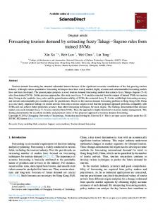
of transportation cost may introduce multicolinearity when employed jointly with overall price indices
156
(Song et al. , 2009).
157
Taking a look at Figure 1, which displays the evolution of tourism demand to Paris for the five source
158
markets, one can infer the following. Tourism demand from all source markets features a distinct seasonal
159
pattern. Whereas the German, Italian, UK and US markets are characterized by clear beginning-of-the-
160
year troughs, this phenomenon is not as prominent for the Japanese market. The US market shows a
161
single summer peak followed by a smaller fall peak, whereas the other source markets display multiple
162
peaks alternating with smaller troughs throughout the year. The Italian source market features a distinct
163
holiday-season peak at the end of the year, which is followed immediately by the beginning-of-the-year-
164
trough. All source markets besides the UK market are characterized by an upswing at the beginning of
165
the sample. The Japanese, the UK and the US markets are further characterized by a slight recovery at the
166
end of the sample, thereby reversing a temporary downward trend, which was amplified in the financial
167
crisis years of 2008 and 2009. The same is true also for the German market, albeit to a lesser extent.
168
The Italian market features the most pronounced downward trend, which is still present at the end of the
169
sample.
7
170
Concerning the various explanatory variables (which are not shown here for reasons of brevity but which
171
are available on request), all own and competing destination price variables are characterized by trend-
172
ing and seasonal behavior as well, although the seasonality effects are not as prominent as they are for
173
tourism demand. The tourist income variable, which by construction is only trending but not affected by
174
seasonality, shows the well-known troughs in real GDP in the crisis years of 2008 and 2009. Except for
175
Italy, where real GDP levels at the end of 2012 are lower than those at the beginning of 2003, all other
176
economies seem to have gradually recovered from the crisis, at least in terms of real GDP. This suggests
177
that Italy remains in “(euro) crisis mode” until the end of the sample.
Figure 1: Evolution of tourism demand Q_DE
Q_IT
11.4
11.6
11.2 11.4 11.0 10.8
11.2
10.6
11.0
10.4 10.8 10.2 10.6
10.0 03
04
05
06
07
08
09
10
11
12
03
04
05
06
Q_JP
07
08
09
10
11
12
09
10
11
12
Q_UK
11.4
12.0
11.2
11.8
11.0
11.6
10.8 11.4 10.6 11.2
10.4 10.2
11.0
10.0
10.8 03
04
05
06
07
08
09
10
11
12
09
10
11
12
03
04
05
06
07
08
Q_US 12.4
12.0
11.6
11.2
10.8
10.4 03
04
05
06
07
08
Source: TourMIS. All values are given in natural logarithms.
178
Since the variables are characterized by time trends and seasonal patterns (apart from the income vari-
8
179
ables which are retrieved already deseasonalized), in addition to non-stationarity, attention has to be
180
given to the possibility of stochastic seasonality. This means that seasonal and non-seasonal means of
181
the data may not be time-constant in the original data. Employing seasonal dummies to capture sea-
182
sonal patterns without proper differencing, thereby mistakenly treating seasonality as deterministic, may
183
decrease a model’s forecasting performance (Shen, Li, and Song, 2009). Consequently, tests on (sea-
184
sonal) unit roots are employed: the Augmented Dickey-Fuller (ADF) test for the non-seasonal unit root
185
in case of tourist income and the monthly version of the Hylleberg-Engel-Granger-Yoo (HEGY) test
186
(Hylleberg, Engle, Granger, and Yoo, 1990), which was developed by Beaulieu and Miron (1993), for
187
seasonal and non-seasonal unit roots in case of all other variables.
188
The null hypothesis of the monthly HEGY test is that all unit roots (the non-seasonal unit root at fre-
189
190
quency 0 and the seasonal unit roots at frequencies π, ± π2 , ∓ 2π , ± π3 , ∓ 5π , ± π6 ) are present. The correspond3 6 √ √ √ √ ing (seasonal) unit roots are 1, −1, ±i, − 12 (1± 3i), 12 (1± 3i), − 21 ( 3±i), 12 ( 3±i), thereby corresponding
191
to j = 0, 6, 3, 9, 8, 4, 2, 10, 7, 5, 1, 11 cycles per year (Beaulieu and Miron , 1993).
192
As can be seen from Table 1, the null hypothesis of the presence of a unit root at frequency 0 cannot be
193
rejected for any of the variables (ADF and HEGY test results). Furthermore, apart from qU K,t , p JP,t , pcJP,t ,
194
the HEGY test results indicate that for all other variables the null hypothesis of the presence of seasonal
195
unit roots cannot be rejected for at least one seasonal frequency. Consequently, some type of filtering has
196
to be applied to the data to assure stationarity. Since filtered data has to remain interpretable, applying the
197
seasonal differencing filter D12 = (1− L12 ) (with D12 , L12 denoting the seasonal differencing and backshift
198
operators, respectively) is proposed as it transforms all the logged variables in conveniently interpretable
199
approximate year-on-year growth rates with the caveat that both trending behavior and seasonal patterns
200
of the original data and the information contained therein are lost after this procedure. Altogether, apply-
201
ing the seasonal differencing filter leaves 108 observations from 2004M1 − 2012M12 per variable and
202
source market for further analysis. Additional ADF tests on the seasonally differenced data lead to the
203
rejection of the null hypothesis of the presence of the non-seasonal unit root for all variables rendering
204
them integrated of order zero (I(0)) so that no further non-seasonal differencing is necessary to obtain
205
stationarity.
9
Table 1: ADF and HEGY test results Variable
Lag order pˆ
Frequencies 0
∓ 2π 3
∓ 5π 6
π
± π2
7.7759∗∗ 9.2701∗∗∗ 4.6757 10.1364∗∗∗ 5.5863∗ 8.5254∗∗∗ 7.6777∗∗ 14.2864∗∗∗ 3.4610 6.7004∗∗ ∗∗∗ ∗ ∗∗∗ 9.1881 5.5868 8.3356 4.9100 7.1646∗∗ ∗∗ ∗∗∗ ∗∗∗ ∗∗ 5.4259 12.1052 10.7560 7.9995 12.1657∗∗∗ 4.5735 5.1729 6.0398∗ 5.3333∗ 3.2441
qDE,t qIT,t q JP,t qUK,t qUS ,t
3 1 1 1 1
−2.9323 −2.4051 −1.8156 −2.1285 −1.4348
−2.6427∗ −1.6783 −2.2008 −2.8694∗∗ −1.5593
pDE,t pIT,t p JP,t pUK,t pUS ,t
2 3 1 2 2
−1.9145 −2.0376 −1.2883 −1.6496 −1.1373
−0.7007 4.8085 −3.6780∗∗∗ 4.8925 −3.7180∗∗∗ 8.9048∗∗∗ −1.5101 4.2734 −2.0444 9.1181∗∗∗
pcDE,t pcIT,t pcJP,t pcUK,t pcUS ,t
2 1 1 2 2
−2.5834 −1.7377 −1.3211 −1.3814 −1.1603
−2.0998 7.2904∗∗ 9.0492∗∗∗ −2.9360∗∗ 9.4948∗∗∗ 11.5519∗∗∗ −3.4785∗∗∗ 8.6557∗∗∗ 6.3527∗∗ −1.3157 4.5844 5.0345 −1.9908 8.9883∗∗∗ 6.3006∗∗
yDE,t yIT,t y JP,t yUK,t yUS ,t
3 3 0 3 3
−2.5402 −1.9836 −2.1040 −2.3264 −2.5207
4.0047 6.1822∗ 5.9112∗ 4.6289 6.2261∗
± π3
± π6
4.1569 4.1690 6.7142∗∗ 5.5869∗ 8.6488∗∗∗ 5.6253∗ 6.4946∗∗ 4.5013 8.6092∗∗∗ 11.7039∗∗∗
4.7124 5.8611∗ 5.5586∗ 7.3134∗∗ 9.1474∗∗∗
7.8776∗∗ 7.3353∗∗ 4.7823 6.7934∗∗ ∗∗∗ 8.8417 5.7265∗ ∗∗ 6.5692 5.4382∗ ∗∗ 7.6666 12.3072∗∗∗
5.8003∗ 7.0001∗∗ 5.7257∗ 7.9948∗∗ 9.0480∗∗∗
Source: TourMIS, OECD, Eurostat, own calculations. All individual tests (HEGY and ADF) include an intercept term and a time trend (estimated coefficients not shown here). In addition, the HEGY tests include seasonal dummy variables (estimated coefficients not shown here). (∗∗∗ ) denotes statistical significance at the 1%, (∗∗ ) at the 5% and (∗ ) at the 10% level. The critical values for the monthly HEGY test (individual t-statistics for frequency π, joint F-statistics for frequencies other than 0 or π) have been tabulated, e.g., by Beaulieu and Miron (1993). The optimal lag order pˆ for each test is determined by BIC.
10
206
Since all variables for all source markets are integrated of order one (I(1)) in levels, it is worthwhile to test
207
whether there are cointegration relationships (CR) between the variables per source market, as planners at
208
DMOs and policy makers may also be interested in the long-run behavior of tourists (Song et al. , 2009).
209
If CRs are found to be present, the long-run equilibrium relationship between the I(1) variables in levels
210
can be estimated by OLS, delivering consistent estimates for the long-run coefficients, yet with distorted
211
standard errors. The short-run dynamics, in turn, can then be modeled by an appropriate (vector) ECM
212
(VECM), which can also be used for forecasting.
213
With the destination’s own price, competing destination prices and tourist income, there are more than
214
two explanatory variables per source market. Therefore, the Johansen maximum likelihood (JML) coin-
215
tegration method is applied (Johansen , 1991, 1995; Song et al. , 2009). As can be seen from Table 2,
216
for the source markets of Germany, Japan, the United Kingdom and the United States, the trace statistics
217
reject the null hypothesis of no cointegration at least at the 5% significance level and one CR per source
218
market is confirmed. However, no CR can be found for the Italian source market and a separate test at
219
the 10% significance level for Italy (not shown here) does not alter this result.
220
3. Rival forecast models
221
The na¨ıve-1 or absolute no change model, which assumes that the forecast value of a variable in period t
222
223
is equal to its realized value in period t − 1 (one-step-ahead forecasting), serves as a natural benchmark forecast model: D12 qˆ i,t = D12 qi,t−1 ,
(1)
224
where the “hatted” variable corresponds to the forecast value. Concerning univariate or pure time-
225
series forecast models, members of the ARIMA and the ETS (Error-Trend-Seasonal or ExponenTial
226
Smoothing, Hyndman et al. , 2002, 2008) model classes are employed. Those have been chosen since
227
Athanasopoulos et al. (2011) find that based on 366 monthly tourism time series, SARIMA and ETS
228
models are able to outperform the seasonal na¨ıve benchmark in terms of predictive accuracy. As the
229
data employed in this study are deseasonalized and I(0) after having applied seasonal differencing, only
11
Table 2: JML cointegration test results Source market
Hypothesized no. of CRs
Eigenvalue
Trace statistic
5% critical value
1% critical value
Germany
Indicated no. of CRs
Lag order pˆ (level eq.)
None At most 1 At most 2 At most 3
0.2912 0.1029 0.0514 0.0098
60.8039 20.1970 7.3859 1.1616
47.21 29.68 15.41 3.76
54.46 35.65 20.04 6.65
1∗∗∗
2
Italy
None At most 1 At most 2 At most 3
0.1854 0.0897 0.0798 0.0000
44.3369 20.5566 9.6517 0.0048
47.21 29.68 15.41 3.76
54.46 35.65 20.04 6.65
0
4
Japan
None At most 1 At most 2 At most 3
0.4007 0.0535 0.0392 0.0005
72.2840 11.3490 4.8063 0.0539
47.21 29.68 15.41 3.76
54.46 35.65 20.04 6.65
1∗∗∗
1
United Kingdom
None At most 1 At most 2 At most 3
0.1938 0.1260 0.0596 0.0187
51.2197 25.5791 9.5564 2.2435
47.21 29.68 15.41 3.76
54.46 35.65 20.04 6.65
1∗∗
1
United States
None At most 1 At most 2 At most 3
0.1703 0.1356 0.0541 0.0145
47.9121 25.6979 8.3565 1.7376
47.21 29.68 15.41 3.76
54.46 35.65 20.04 6.65
1∗∗
1
Source: TourMIS, OECD, Eurostat, own calculations. All JML cointegration tests include orthogonalized sesonal dummy variables as suggested by Johansen (1995) to capture seasonal patterns in the data while not distorting the trace test statistics. In line with Song and Witt (2000) it is assumed that the data are subject to a linear deterministic trend while the cointegration equation itself only includes an intercept. The number of CRs as indicated by the trace statistics per source market is given in column no. 7. (∗∗∗ ) denotes rejection of the null hypothesis of no cointegration at the 1% and (∗∗ ) at the 5% level. The critical values have been tabulated by Osterwald-Lenum (1992). The optimal lag order pˆ for the vector-autoregressions in first differences for each cointegration test is determined by BIC.
12
230
ARMA and ETS models suited for non-seasonal and stationary data are relevant in this study.
231
The (S)AR(I)MA model class as proposed by Box and Jenkins (1970) has been extensively employed in
232
the tourism demand forecasting literature. Pertaining to the numerous studies that employ these models
233
published in 2000 and thereafter (Song et al. , 2009), the majority has used them as benchmark models
234
when assessing the forecast accuracy of more complex multivariate models (e.g. Kulendran and Witt ,
235
2001; Li et al. , 2006; Song, Romilly, and Liu, 2000; Witt, Song, and Louvieris, 2003). A standard ARMA
236
(p, q) reads as follows: ϕ(L)D12 qi,t = α + ϑ(L)υi,t ,
(2)
237
where ϕ(L), ϑ(L) denote lag polynomials of lag orders p and q respectively, α an intercept term, and
238
υi,t denotes an error term to be i.i.d. ∼ N(0, σ2υi ). Eq. (2) can be estimated by using OLS. In a first
239
step, an attempt is made to determine the optimal lag orders p, ˆ qˆ for the single source markets by visual
240
inspection of the autocorrelation and partial autocorrelation functions of D12 qi,t . For the source markets
241
of Italy and Japan, this inspection suggests the use of AR(1) specifications in both cases, which is also
242
backed by automatic model selection based on the Bayesian information criterion (BIC). However, visual
243
inspection for the remaining three source markets reveals a somewhat more complex ARMA structure,
244
where a clear AR(p) or MA(q) specification is not clearly distinguishable. Therefore, automatic model
245
selection based on BIC is employed, thereby suggesting an ARMA(2,1) specification for the source
246
markets of Germany and the United States and an ARMA(1,1) specification for the source market of the
247
United Kingdom.
248
The ETS model class was developed by Hyndman et al. (2002, 2008) and encompasses various ex-
249
ponential smoothing methods such as single or double exponential smoothing or variants of the Holt
250
and Holt-Winters methods within a theoretically founded state-space framework which is estimated re-
251
cursively by employing maximum-likelihood methods. With the exception of Athanasopoulos et al.
252
(2011), this model class has not been applied to tourism demand forecasting very often. Examples for
253
tourism forecasting studies employing traditional exponential smoothing methods published in 2000 and
254
thereafter include Cho (2001); Law (2000); Veloce (2004), where, similar to the AR(I)MA(X) mod-
255
els, expontential smoothing models have been mostly used as benchmarks when assessing the forecast
13
256
accuracy of more complex multivariate models. The ETS framework consists of a signal equation for
257
the forecast variable and a number of state equations for the components that cannot be observed (level,
258
trend, seasonal, Hyndman and Athanasopoulos , 2013, section 7/7). Since the present data are given in
259
logs and have been deseasonalized and stationarized, the appropriate ETS model is ETS(A, N, N) with
260
Additive error, No trend component and No seasonal component, thereby corresponding to classical
261
single-exponential smoothing. In state-space form, ETS(A, N, N) reads: D12 qi,t = li,t−1 + υi,t , li,t = li,t−1 + γυi,t ,
262
263
(3) (4)
with Eq. (3) representing the signal equation, Eq. (4) the state equation, lt denoting the unobservable level component, γ with 0 ≤ γ ≤ 1 the smoothing parameter, and υi,t denoting an error term to be i.i.d.
264
∼ N(0, σ2υi ) appearing in both the signal and the state equation (Hyndman and Athanasopoulos , 2013,
265
section 7/7, so-called single-source-of-error model). The estimation of the system of Eqs. (3) and (4) is
266
undertaken by employing maximum-likelihood methods.
267
According to Song and Li (2008), most studies in forecasting tourism demand based on monthly data
268
only employ univariate models. Table 3 suggests, however, that for the present dataset the use of addi-
269
tional variables can be useful in terms of an increase in predictive accuracy for all source markets based
270
on block Granger causality tests. The test results are based on unconstrained vector autoregressions
271
(VAR) with intercepts estimated by OLS with optimal lag orders of pˆ = 1 as determined by BIC and
272
pˆ = 12 as determined by Akaike’s information criterion (AIC), respectively (L¨utkepohl , 2006). The
273
null hypothesis of the block Granger causality test with tourism demand as dependent variable is that
274
all explanatory variables jointly do not Granger cause tourism demand and hence are not beneficial to
275
its prediction. This hypothesis is rejected across source markets, albeit only for the VAR(1) in the case
276
of Italy. In conclusion, employing explanatory variables may generally prove worthwhile in terms of
277
increasing predictive accuracy.
278
Given that monthly data are employed, an impact of past realizations of the explanatory variables on
279
current realizations of tourism demand is also likely since potential tourists usually observe prices and 14
280
exchange rates and receive income before they decide to travel, at least in case of private visitors. Further-
281
more, the inclusion of past realizations of the dependent variable itself allows behavioral patterns such as
282
habit persistence or tourism expectations to be taken into account (Song et al. , 2003b).
283
One multivariate model that allows for past realizations of the dependent variable as well as current and
284
past realizations of the explanatory variables is ADLM. As noted by Song et al. (2009), Engle and Granger
285
(1987) show that for cointegrated variables every ADLM can be rewritten as an ECM, which means
286
that formulating an ADLM or an ECM are just two different ways of formulating the same model.
287
Song et al. (2009) even present further advantages estimating this so-called error-correction formula-
288
tion of the ADLM (EC-ADLM) has relative to estimating the model in traditional ADLM notation. For
289
the present article, this is particularly convenient since the ADLM can then also be written in terms of
290
seasonally differenced variables, which is the same way the remaining forecast models have been formu-
291
lated. Apart from the Italian source market, one CR per source market could be confirmed by the JML
292
method so that applying EC-ADLM is justifiable for the given data (see Table 2). The first author to
293
employ an ECM for tourism demand forecasting was Kulendran (1996). In the past ten years this model
294
class has become more popular in tourism demand forecasting (Li et al. , 2006; Song et al. , 2003a,b,
295
2013, are some recent examples). Allowing for seasonal lags of the dependent and explanatory variables
296
in levels only results in the subsequent reduced ADLM: qi,t = α0 + α1 pi,t + α2 pci,t + α3 yi,t + β1 pi,t−12 + β2 pci,t−12 + β3 yi,t−12 + ϕqi,t−12 + υi,t .
(5)
297
Subtracting qi,t−12 from both sides of Eq. (5) and some further manipulation yields the following EC-
298
ADLM: D12 qi,t = α0 + α1 D12 pi,t + α2 D12 pci,t + α3 D12 yi,t + (α1 + β1 )pi,t−12 + (α2 + β2 )pci,t−12 + (α3 + β3 )yi,t−12 − (1 − ϕ)qi,t−12 + υi,t ,
299
(6)
where α j for j ∈ {1, 2, 3} are called impact parameters, −(1−ϕ) with −1 < −(1−ϕ) < 0 is called coefficient
300
of the error correction term (Song et al. , 2009), and υi,t denotes an error term to be i.i.d. ∼ N(0, σ2υi ).
301
Eq. (6) can be estimated by using OLS and is employed as one of the rival forecast models. For all five 15
302
source markets, the estimated coefficients of the error correction terms feature the expected negative sign
303
(not shown here) so that convergence to the long-run equilibrium relationships between the variables in
304
levels is ensured.
305
Another conclusion that can be drawn from Table 3 is that none of the explanatory variables should be
306
regarded as exogenous, except for tourist income in Germany, competing destination prices for the UK
307
market, as well as own and competing destination prices for the US market. This assumption is sup-
308
posed to hold when either static regression or (EC-) ADLM are employed as forecast models. Moreover,
309
preliminary recursive estimation of multivariate regression models employing the Kalman (1960) filter
310
algorithm has revealed that the assumption of time-constant parameters, which is one of the additional
311
assumptions to be fulfilled for static regression or (EC-) ADLM estimation (e.g. Song et al. , 2003a),
312
does not hold for any of the income elasticities for all source markets, as can be seen from Figure 2.2
313
This is why static regression, which is neither able to capture the dynamics (unlike (EC-) ADLM) nor
314
the somewhat more complex mutual causality structure and variability of the parameter estimates in the
315
data, was discarded as potential rival forecast model. Employing it nonetheless, most likely, would have
316
resulted in a non-satisfactory forecasting performance (Song et al. , 2009).
317
Fluctuations of elasticities are stronger at the beginning of the sample than at the end of the sample (even
318
stronger fluctuations during 2004 are omitted for legibility reasons. After about 2010, the elasticities for
319
the German, Italian and Japanese markets usually hover between 1 and 2 and for the UK market around
320
3, thereby indicating that a trip to Paris can be deemed a luxury good. In the case of the US market,
321
after being characterized by a positive tourist income elasticity at the beginning of the sample, slightly
322
negative values are attained from 2010 onward. However, these values are not significantly different from
323
zero.
324
As a consequence, multivariate models that relax the assumptions of parameter constancy and exogeneity 2 Graphs showing the time-varying elasticities of the remaining explanatory variables are not shown here for reasons of brevity but are available on request; apart from the elasticity with respect to the own price variable on the Italian source market, all elasticities are characterized by the expected sign for the major part of the sample.
16
Figure 2: Time-varying elasticities of tourism demand with respect to tourist income ALPHA_3_DE
ALPHA_3_IT
4
12 10
0
8 -4 6 -8 4 -12
2 0
-16 2005
2006
2007
2008
2009
2010
2011
2012
2005
2006
2007
ALPHA_3_JP
2008
2009
2010
2011
2012
2010
2011
2012
ALPHA_3_UK
4
5
3
4
2
3
1
2
0
1
-1
0
-2
-1 -2
-3 2005
2006
2007
2008
2009
2010
2011
2012
2010
2011
2012
2005
2006
2007
2008
2009
ALPHA_3_US 16
12
8
4
0
-4 2005
2006
2007
2008
2009
Source: TourMIS, OECD, Eurostat, own calculations.
17
Table 3: Block Granger causality test results Dependent variable
Excluded variables
D12 qDE,t D12 pDE,t D12 pcDE,t D12 yDE,t
All other German All other German All other German All other German
D12 qIT,t D12 pIT,t D12 pcIT,t D12 yIT,t
All other Italian All other Italian All other Italian All other Italian
D12 q JP,t D12 p JP,t D12 pcJP,t D12 y JP,t
pˆ = 1 (BIC)
pˆ = 12 (AIC)
7.0934∗ 11.0720∗∗ 2.7188 0.9224
54.4666∗∗ 62.0689∗∗∗ 68.2511∗∗∗ 40.7788
7.9035∗∗ 5.4747 2.5520 8.6926∗∗
27.4169 80.9547∗∗∗ 90.7958∗∗∗ 87.4107∗∗∗
All other Japanese All other Japanese All other Japanese All other Japanese
8.4853∗∗ 15.2051∗∗∗ 17.4947∗∗∗ 8.1227∗∗
60.7593∗∗∗ 98.1206∗∗∗ 94.2001∗∗∗ 172.3678∗∗∗
D12 qUK,t D12 pUK,t D12 pcUK,t D12 yUK,t
All other UK All other UK All other UK All other UK
8.9780∗∗ 8.0423∗∗ 5.9536 11.6779∗∗∗
72.5357∗∗∗ 45.4485 42.9208 39.2774
D12 qUS ,t D12 pUS ,t D12 pcUS ,t D12 yUS ,t
All other US All other US All other US All other US
7.0092∗ 0.3482 0.3265 4.4071
85.8122∗∗∗ 40.6233 35.7715 53.4686∗∗
Source: TourMIS, OECD, Eurostat, own calculations. (∗∗∗ ) denotes statistical significance of the χ2 statistics at the 1%, (∗∗ ) at the 5% and (∗ ) at the 10% level. The optimal lag order is determined by BIC ( pˆ = 1, degrees of freedom: 3) and AIC ( pˆ = 12, degrees of freedom: 36), respectively.
18
325
of the explanatory variables are employed as well. A multivariate model which relaxes the assumption of
326
exogeneity of the explanatory variables is the VAR(p) approach favored by Sims (1980) and first intro-
327
duced to tourism demand forecasting by Kulendran and King (1997); Kulendran and Witt (1997). Re-
328
cent examples of VAR(p) application in tourism demand forecasting include Lim and McAleer (2001);
329
Oh (2005); Shan and Wilson (2001); Song and Witt (2006), whereby Shan and Wilson (2001) employ
330
monthly data. In its general form it reads: Xi,t = Ai,t + Φ1 Xi,t−1 + Φ2 Xi,t−2 + ... + Φ p Xi,t−p + Υi,t ,
(7)
331
where Ai,t is a k×1 vector of intercept terms, Xi,t a k×1 vector of the observed variables per source market
332
(D12 qi,t , D12 pi,t , D12 pci,t , D12 yi,t ), Φ a k × k coefficient matrix, and Υi,t a k × 1 vector of error terms to be
333
i.i.d ∼ N(0, ΣΥi ). Since the error terms are assumed to be contemporaneously but not serially correlated,
334
Eq. (7) can be estimated using OLS (e.g. Song et al. , 2003a). As indicated above, the optimal lag order
335
pˆ is selected by BIC ( pˆ = 1) and AIC ( pˆ = 12). While the advantage of a higher lag order as selected
336
by AIC is that the dynamics of the data-generating process may be better captured, its disadvantage – at
337
least concerning unconstrained VAR estimation by OLS or pure maximum likelihood – is that highly or
338
even over-parameterized models would have to be estimated, which in turn would be detrimental to their
339
forecasting performance. This indeed was the case during a preliminary forecast evaluation based on an
340
unconstrained VAR(12) model estimated by OLS, which was only seldom able to outperform the na¨ıve-1
341
benchmark, while the VAR(1) model performed quite well. Since the dynamics of the VAR(1) and the
342
VAR(12) models differ quite substantially, as can be seen from Table 3, the questions remains of how to
343
cope with this issue.
344
One way to circumvent the relatively poor forecasting performance of a VAR with a high lag order, is
345
to employ Bayesian methods rather than pure maximum likelihood or OLS. In doing so, the so-called
346
Minnesota or Litterman prior for Bayesian VAR (BVAR) estimation and forecasting is employed. The
347
Minnesota prior is an informative prior developed by and specified in Doan, Litterman, and Sims (1984)
348
on an otherwise unconstrained VAR with intercept, which imposes restrictions on the more distant lags
349
of a VAR rather than eliminating them. In the tourism demand forecasting literature, this model was first
19
350
introduced by Wong et al. (2006), but has been only rarely employed thereafter (e.g. Song et al. , 2013).
351
As laid out, e.g., in L¨utkepohl (2006), for Bayesian estimation it is assumed that non-sample informa-
352
tion on a generic parameter vector ψ available prior to estimation is summarized in its prior probability
353
density function (PDF) g(ψ). The sample information on ψ, however, is summarized in its sample PDF
354
given by f (y|ψ), which is algebraically identical to the likelihood function l(ψ|y). The distribution of the
355
parameter vector ψ conditional on the sample information contained in y can be summarized by g(ψ|y),
356
which is known as posterior PDF. The posterior distribution, which contains all information available
357
for the parameter vector ψ, is proportional to the likelihood function times the prior PDF and has to be
358
obtained numerically. For the present case, the parameter vector ψ mainly consists of the three BVAR
359
hyperparameters: overall tightness (set to 0.1, denoting a relatively tight value as recommended for small
360
BVAR systems), relative cross-variable weight (set to 0.5, reflecting symmetric characteristics of the
361
BVAR model), and lag decay (set to 1, representing linear decay), which are meant to obtain a model
362
that is referred to as a “standard BVAR” in Wong et al. (2006). Consequently, VAR(1), BVAR(1) and
363
BVAR(12) models are employed as forecast models for all five source markets.
364
Another multivariate model which in turn relaxes the assumption of parameter constancy, and was there-
365
fore suggested by Engle and Watson (1987) for use in the presence of structural instability, is the TVP
366
model which was first introduced to tourism demand forecasting by Riddington (1999). In recent years,
367
the TVP approach has been employed, e.g., by Li et al. (2006); Song et al. (2003a,b); Song and Wong
368
(2003). However, the TVP model treats all explanatory variables as exogenous and by construction does
369
not permit past realizations of both the dependent and the explanatory variables to have an impact on the
370
current realization of the dependent variable. In its general form it reads: D12 qi,t = α0,i,t + α1,i,t D12 pi,t + α2,i,t D12 pci,t + α3,i,t D12 yi,t + υi,t , α j,i,t = α j,i,t−1 + ε j,i,t ,
(8) (9)
371
where Eq. (8) denotes the signal equation and Eq. (9) the j = 0, ..., 3 state equations of the TVP model,
372
one for each of the four time-varying parameters (Song and Wong , 2003). The form of the state equation
373
is a random walk, thereby corresponding to the most commonly used specification of a state equation in 20
374
TVP estimation (Song et al. , 2003a). υi,t and ε j,i,t are error terms to be i.i.d. ∼ N(0, σ2υi ) and ∼ N(0, σ2εi )
375
and not to be correlated with each other. The estimation of the system of Eqs. (8) and (9) is taken out by
376
employing the Kalman (1960) filter algorithm.
377
An additional feature of the TVP model is that its recursive estimation technique, where more recent
378
information has a higher impact than information from the distant past, is able to capture structural
379
changes in the data such as the onset of the financial crisis in the US in late 2007, which started fully
380
unfolding in the US, Europe and other parts of the world in 2008 only (Song et al. , 2003a).
381
One possibility to accommodate such structural changes within EC-ADLM and (Bayesian) VAR ap-
382
proaches would be the inclusion of dummy variables. For the present case, however, the addition of a
383
crisis dummy attaining the value 1 from 2008M4 onward and 0 otherwise (since in this month the year-
384
on-year real GDP growth rates of Italy and Japan turned negative for the first time, soon after followed
385
by the three remaining source markets) would lead to a marginal improvement over a BVAR(1) model
386
without the crisis dummy only in the case of the Italian source market, which may be due to Italy still
387
being in “(euro) crisis mode” at the end of the sample (see Section 2).
388
Since preliminary inclusion of a crisis dummy has almost always led to a deterioration of forecasting
389
accuracy for the remaining vector autoregressive specifications and the other source markets, and for
390
reasons of consistency among model specifications across source markets, crisis dummy variables were
391
discarded from the rival forecast models. Concerning EC-ADLM, apart from the US source market, the
392
crisis dummy turned out to be statistically insignificant in the first place.
393
4. Forecast evaluation
394
The forecast evaluation procedure is carried out as follows. The forecasting performance of the seven ri-
395
val forecast models is evaluated with respect to the na¨ıve-1 benchmark for each source market in terms of
396
ex-post out-of-sample predictive means of total arrivals for forecast horizons h = 1, 2, 3, 6, 12, 24 months
397
ahead while using expanding windows. The expanding windows (or recursive) forecasting technique,
398
which expands the estimation window by one observation for each forecast roll, introduces another di21
399
mension of variability to the forecast evaluation procedure for the different forecast models in addition to
400
different source markets and forecast horizons. In addition, using expanding windows also corresponds
401
to a “natural” practitioner’s situation, where all information available up to the forecast origin is used
402
for forecasting. In case of multivariate models, actual values of the explanatory variables are employed
403
(ex-post forecasting). This means the multivariate models incorporate extra information, which could
404
potentially boost predictive ability, that is not available to time-series models.
405
406
Each forecast model is re-estimated on a monthly basis starting with sub-sample 2004M1 − 2009M12 (72 observations) up to 2004M1 − 2012M11 (107 observations for h = 1), ..., 2004M1 − 2010M12 (90
407
observations for h = 24), respectively. Altogether, this delivers T 1 = 36 (for h = 1), ..., T 24 = 13 (for
408
h = 24) counterfactual observations per model and source market since the forecast window is set to the
409
period 2010M1 − 2012M12.
410
As measures of forecasting accuracy, the traditional root mean squared error (RMSE) and mean absolute
411
error (MAE) are employed, of which the latter is more sensitive to small deviations from zero, but less
412
sensitive to large deviations since it is not computed based on squared losses. Calculating the RMSE
413
and MAE for logged variables, as done in the present research, has the additional property that these
414
measures approximately correspond to the RMSPE and MAPE of the untransformed variables. The
415
RMSE and MAE values per source market, forecast model and forecast horizon including rankings from
416
1 (best model) to 8 (worst model) are given in Tables 4 (shorter horizons: h = 1, 2, 3) and 5 (longer
417
horizons: h = 6, 12, 24). The respective best-performing models are given in boldface.
418
In addition, the Hansen test on superior predictive accuracy is employed to investigate if the na¨ıve-1
419
benchmark is statistically significantly outperformed by at least one of the seven competing forecast
420
models (Hansen , 2005). The null hypothesis of the Hansen test is that a benchmark forecast model
421
(in the present case: the na¨ıve-1 model) is not outperformed by any other forecast model. The Hansen
422
consistent p-values, which are also reported in Tables 4 and 5, are consistent insofar as the Hansen
423
test procedure asymptotically prevents all forecast models that are worse than the benchmark model
424
from having an impact on the estimated distribution of the Hansen test statistic itself. Boldface Hansen
425
consistent p-values indicate a statistically significant outperformance of the na¨ıve-1 benchmark at least at
22
426
the 10% level. Due to the limited number of observations available, these tests have not been evaluated
427
for the forecast horizon h = 24. All calculations are performed with the MulCom package for Ox
428
(Hansen and Lunde , 2010) while assuming squared forecast losses to be minimized in the loss function.
429
Table 4 shows the results of accuracy tests for the short forecast horizons. The accuracy of the forecast
430
models differs according to the source market. For instance, for Germany VAR(1), Italy BVAR(12),
431
Japan AR(1), the United Kingdom ARMA(1,1), and the United States ETS(A, N, N) are most frequently
432
the models with the smallest errors across forecast horizons and error measures.
433
The results for longer term forecasting are given in Table 5. Visitors from Italy are best forecast with
434
BVAR(12), from the UK with VAR(1), and from the US with ETS(A, N, N) in general. For the German
435
and Japanese source markets, however, the results are mixed and for each forecast horizon a different
436
model performs best.
437
Pertaining to the significant outperformance of the na¨ıve-1 benchmark according to the Hansen test, it
438
can be seen from Tables 4 and 5 that apart from three exceptions (the German market for h = 3, and
439
the Japanese and UK markets for h = 1) the outperformance of the na¨ıve-1 benchmark is statistically
440
significant across nearly all source markets and forecast horizons. As stated, the test statistics have not
441
been calculated for forecast horizon h = 24 due to the limited number of observations available.
442
For forecasting German tourist arrivals to Paris, the VAR(1) model is generally more accurate than other
443
models applied in this study, followed by BVAR(1). To predict two or three months ahead, VAR(1) can
444
be used, whereas to predict longer term forecasting of German tourists such as six to twelve months
445
ahead, BVAR(1) and VAR(1) are both better than other models. For forecasting two years ahead, TVP is
446
more accurate than its competitors.
447
For predicting Italian tourist arrivals in the short term, BVAR(12) outperforms all the other models in
448
terms of having the smallest RMSE over all forecast horizons from one to three months ahead. For longer
449
term forecasting (six, twelve and twenty-four months ahead), BVAR(12) and ETS(A, N, N) outperform
450
the other models.
23
451
Japanese tourists seem to be hard to predict concerning their tourism demand to Paris. Overall, VAR(1)
452
performs well for both short and longer term forecasting. However, there are some exceptions to this. For
453
predicting one month ahead, AR(1) or ETS(A, N, N) work best and for predicting twelve months ahead
454
AR(1) outperforms others.
455
UK tourists are easier to predict in the short term, since ARMA(1,1) outperforms all the others for
456
forecasting up to six months ahead. In the longer term (forecasting twelve months and two years ahead),
457
VAR(1) is the most accurate forecast model. For forecasting six months ahead, ARMA(1,1) performs
458
best.
459
For predicting US tourist arrivals to Paris in general, ETS(A, N, N) performs better than the other models
460
both in the short and in the longer term. However, when predicting two years ahead, VAR(1) outperforms
461
all the other models.
462
The significant outperformance of the na¨ıve-1 benchmark in many occasions is worth noting since this is
463
a non-standard result, especially because all rival forecast models perform similarly well in most cases.
464
One possible explanation for this could be common features in the data, such as trends and seasonal
465
patterns, which the na¨ıve-1 benchmark is not able to capture. However, since all variables had been
466
detrended and deseasonalized (stationary data) before they entered the forecasting competition, this ex-
467
planation does not hold.
468
A more likely explanation is the use of the expanding windows (or recursive) forecasting technique.
469
Based on Monte Carlo simulations, Pesaran and Pick (2011) find that averaging forecasts over different
470
estimation windows almost always leads to a lower RMSE relative to forecasts that are based on single
471
estimation windows, even in the presence of structural breaks. The authors confirm this general result by
472
an application to financial data. Since the na¨ıve-1 benchmark cannot benefit from the information gained
473
from using expanding estimation windows by construction, it is believed that this forecasting techniques
474
is one likely source for statistically significant outperformance of the benchmark.
475
Concerning the overall good performance of multivariate models even if outperformed by univariate
476
models for the US and UK source markets, it is believed that the employed multivariate forecast models, 24
477
(B)VAR and TVP, are the ones that are able to capture best important characteristics of the data such as
478
mutual causality between dependent and explanatory variables and time-varying elasticities, respectively.
25
Table 4: RMSE, MAE values and Hansen test results (h = 1, 2, 3) Source market
Forecast model
h=1 RMSE
Rank
MAE
Rank
h=2 RMSE
Rank
MAE
Rank
h=3 RMSE
Rank
MAE
Rank
26
Germany
ARMA(2,1) ETS(A, N, N) EC-ADLM VAR(1) BVAR(1) BVAR(12) TVP Na¨ıve-1 Hansen consistent p-value
0.1370 0.1274 0.1396 0.1233 0.1238 0.1201 0.1346 0.1925 0.0173
6 4 7 2 3 1 5 8
0.1096 0.0983 0.1177 0.0943 0.0934 0.0941 0.0981 0.1488
6 5 7 3 1 2 4 8
0.1241 0.1248 0.1382 0.1199 0.1202 0.1249 0.1313 0.1504 0.0936
3 4 7 1 2 5 6 8
0.0967 0.0978 0.1191 0.0893 0.0927 0.0982 0.0979 0.1203
3 4 7 1 2 6 5 8
0.1308 0.1300 0.1439 0.1198 0.1215 0.1283 0.1366 0.1611 0.1151
5 4 7 1 2 3 6 8
0.1036 0.1022 0.1234 0.0896 0.0935 0.1012 0.0985 0.1251
6 5 7 1 2 4 3 8
Italy
AR(1) ETS(A, N, N) EC-ADLM VAR(1) BVAR(1) BVAR(12) TVP Na¨ıve-1 Hansen consistent p-value
0.0944 0.0955 0.0971 0.0944 0.1081 0.0934 0.1044 0.1213 0.0467
3 4 5 2 7 1 6 8
0.0775 0.0797 0.0826 0.0799 0.0868 0.0773 0.0805 0.0943
2 3 6 4 7 1 5 8
0.0955 0.0988 0.1008 0.1019 0.0980 0.0948 0.1095 0.1214 0.0332
2 4 5 6 3 1 7 8
0.0776 0.0827 0.0839 0.0845 0.0796 0.0782 0.0844 0.0963
1 4 5 7 3 2 6 8
0.0979 0.1014 0.1038 0.1006 0.0998 0.0934 0.1154 0.1245 0.0104
2 5 6 4 3 1 7 8
0.0800 0.0858 0.0844 0.0871 0.0817 0.0765 0.0893 0.1056
2 5 4 6 3 1 7 8
Japan
AR(1) ETS(A, N, N) EC-ADLM VAR(1) BVAR(1) BVAR(12) TVP Na¨ıve-1 Hansen consistent p-value
0.1114 0.1195 0.1443 0.1145 0.1119 0.1126 0.1218 0.1225 0.1610
1 5 8 4 2 3 6 7
0.0942 0.0925 0.1126 0.0953 0.0957 0.0947 0.0974 0.1014
3 1 8 4 5 3 6 7
0.1362 0.1488 0.1432 0.1380 0.1375 0.1477 0.1453 0.1638 0.0764
1 7 4 3 2 6 5 8
0.1106 0.1174 0.1220 0.1003 0.1190 0.1246 0.1153 0.1311
2 4 6 1 5 7 3 8
0.1393 0.1588 0.1505 0.1373 0.1408 0.1567 0.1586 0.1792 0.0376
2 7 4 1 3 5 6 8
0.1166 0.1251 0.1286 0.1056 0.1226 0.1307 0.1301 0.1431
2 4 5 1 3 7 6 8
United Kingdom
ARMA(1,1) ETS(A, N, N) EC-ADLM VAR(1) BVAR(1) BVAR(12) TVP Na¨ıve-1 Hansen consistent p-value
0.0787 0.0790 0.0922 0.0847 0.0902 0.0920 0.0832 0.0889 0.1360
1 2 8 4 6 7 3 5
0.0604 0.0605 0.0689 0.0647 0.0719 0.0710 0.0631 0.0683
1 2 6 4 8 7 3 5
0.0818 0.0834 0.0878 0.0914 0.0991 0.0965 0.0856 0.0997 0.0193
1 2 4 5 7 6 3 8
0.0619 0.0628 0.0691 0.0720 0.0806 0.0757 0.0636 0.0789
1 2 4 5 8 6 3 7
0.0810 0.0830 0.0849 0.0941 0.1027 0.0996 0.0847 0.1015 0.0120
1 2 4 5 8 6 3 7
0.0660 0.0650 0.0648 0.0756 0.0824 0.0787 0.0635 0.0862
4 3 2 5 7 6 1 8
United States
ARMA(2,1) ETS(A, N, N) EC-ADLM VAR(1) BVAR(1) BVAR(12) TVP Na¨ıve-1 Hansen consistent p-value
0.0783 0.0724 0.1051 0.0741 0.0707 0.0722 0.0772 0.0827 0.0488
6 3 8 4 1 2 5 7
0.0593 0.0570 0.0881 0.0608 0.0586 0.0588 0.0590 0.0638
5 1 8 6 2 3 4 7
0.0749 0.0711 0.1123 0.0742 0.0846 0.0825 0.0802 0.0829 0.0075
3 1 8 2 7 5 4 6
0.0594 0.0578 0.0959 0.0575 0.0707 0.0681 0.0630 0.0694
3 2 8 1 7 5 4 6
0.0794 0.0684 0.1204 0.0748 0.0953 0.0899 0.0817 0.0816 0.0020
3 1 8 2 7 6 5 4
0.0608 0.0535 0.1034 0.0625 0.0796 0.0758 0.0617 0.0656
2 1 8 4 7 6 3 5
Source: TourMIS, OECD, Eurostat, own calculations. Minimum RMSE and MAE values per forecast horizon and source market are given in boldface. Boldface Hansen consistent p-values denote rejection of the null hypothesis of no outperformance of the na¨ıve-1 benchmark by at least one competing forecast model at the 10% level or higher. Squared forecast losses are assumed to be minimized when calculating the Hansen statistics.
Table 5: RMSE, MAE values and Hansen test results (h = 6, 12, 24) Source market
Forecast model
h=6 RMSE
Rank
MAE
Rank
h = 12 RMSE
Rank
MAE
Rank
h = 24 RMSE
Rank
MAE
Rank
27
Germany
ARMA(2,1) ETS(A, N, N) EC-ADLM VAR(1) BVAR(1) BVAR(12) TVP Na¨ıve-1 Hansen consistent p-value
0.1311 0.1343 0.1483 0.1252 0.1241 0.1299 0.1344 0.1951 0.0044
4 5 7 2 1 3 6 8
0.1029 0.1050 0.1297 0.0902 0.0938 0.1010 0.0975 0.1507
5 6 7 1 2 4 3 8
0.1394 0.1361 0.1615 0.1342 0.1337 0.1379 0.1460 0.2249 0.0236
5 3 7 2 1 4 6 8
0.1078 0.1047 0.1392 0.0992 0.1016 0.1064 0.1053 0.1581
6 3 7 1 2 5 4 8
0.1345 0.1429 0.1761 0.1192 0.1187 0.1309 0.1176 0.1492
5 6 8 3 2 4 1 8
0.1013 0.1096 0.1525 0.0915 0.0916 0.0991 0.0832 0.1245
5 6 8 2 3 4 1 8
Italy
AR(1) ETS(A, N, N) EC-ADLM VAR(1) BVAR(1) BVAR(12) TVP Na¨ıve-1 Hansen consistent p-value
0.0962 0.1014 0.1025 0.1017 0.0977 0.0932 0.1109 0.1387 0.0007
2 4 6 5 3 1 7 8
0.0784 0.0819 0.0822 0.0840 0.0798 0.0745 0.0876 0.1179
2 4 5 6 3 1 7 8
0.0973 0.0852 0.0952 0.0961 0.0999 0.0882 0.1147 0.1255 0.0038
5 1 3 4 6 2 7 8
0.0770 0.0665 0.0751 0.0757 0.0793 0.0726 0.0893 0.1027
5 1 3 4 6 2 7 8
0.0961 0.0904 0.1016 0.0975 0.0978 0.0896 0.1400 0.1458
3 2 6 4 5 1 7 8
0.0754 0.0630 0.0733 0.0780 0.0768 0.0721 0.1175 0.0958
4 1 3 6 5 2 8 7
Japan
AR(1) ETS(A, N, N) EC-ADLM VAR(1) BVAR(1) BVAR(12) TVP Na¨ıve-1 Hansen consistent p-value
0.1446 0.1724 0.1368 0.1231 0.1467 0.1584 0.1453 0.1893 0.0105
3 7 2 1 5 6 4 8
0.1269 0.1386 0.1147 0.0975 0.1292 0.1356 0.1176 0.1601
4 7 2 1 5 6 3 8
0.1368 0.2126 0.1437 0.1598 0.1368 0.1436 0.1527 0.2385 0.0002
1 7 4 6 2 3 5 8
0.1212 0.1855 0.1277 0.1406 0.1215 0.1255 0.1285 0.2023
1 7 4 6 2 3 5 8
0.1407 0.1199 0.2581 0.1595 0.1448 0.1592 0.1925 0.1428
2 1 8 6 4 5 7 3
0.1273 0.0854 0.2319 0.1446 0.1317 0.1451 0.1787 0.1141
3 1 8 5 4 6 7 2
United Kingdom
ARMA(1,1) ETS(A, N, N) EC-ADLM VAR(1) BVAR(1) BVAR(12) TVP Na¨ıve-1 Hansen consistent p-value
0.0924 0.0949 0.1018 0.1075 0.1119 0.1159 0.1094 0.1113 0.0035
1 2 3 4 7 8 5 6
0.0729 0.0753 0.0779 0.0860 0.0926 0.0970 0.0854 0.0917
1 2 3 5 7 8 4 6
0.1126 0.1301 0.1223 0.1021 0.1230 0.1241 0.1567 0.1423 0.0919
2 6 3 1 4 5 8 7
0.0926 0.1012 0.0969 0.0878 0.1027 0.1030 0.1334 0.1066
2 4 3 1 5 6 8 7
0.1439 0.1998 0.1282 0.1011 0.1503 0.1398 0.2357 0.2103
4 6 2 1 5 3 8 7
0.1336 0.1887 0.1106 0.0802 0.1409 0.1303 0.2293 0.1667
4 7 2 1 5 3 8 6
United States
ARMA(2,1) ETS(A, N, N) EC-ADLM VAR(1) BVAR(1) BVAR(12) TVP Na¨ıve-1 Hansen consistent p-value
0.0931 0.0743 0.1376 0.0920 0.1052 0.1056 0.0897 0.0854 0.0021
5 1 8 4 6 7 3 2
0.0769 0.0617 0.1181 0.0789 0.0889 0.0898 0.0745 0.0726
4 1 8 5 6 7 3 2
0.1231 0.1014 0.1707 0.1057 0.1163 0.1237 0.1079 0.1149 0.0160
6 1 8 2 5 7 3 4
0.1099 0.0746 0.1546 0.0890 0.1017 0.1100 0.0796 0.0880
6 1 8 4 5 7 2 3
0.1670 0.1568 0.2136 0.1144 0.1401 0.1523 0.1911 0.1623
6 4 8 1 2 3 7 5
0.1595 0.1397 0.2082 0.0986 0.1344 0.1467 0.1624 0.1287
6 4 8 1 3 5 7 2
Source: TourMIS, OECD, Eurostat, own calculations. Minimum RMSE and MAE values per forecast horizon and source market are given in boldface. Boldface Hansen consistent p-values denote rejection of the null hypothesis of no outperformance of the na¨ıve-1 benchmark by at least one competing forecast model at the 10% level or higher. Squared forecast losses are assumed to be minimized when calculating the Hansen statistics.
479
5. Conclusions
480
The purpose of this study was to compare the predictive accuracy of various uni- and multivariate models
481
in forecasting international city tourism demand for Paris, which has been Europe’s number one city des-
482
tination in terms of tourist arrivals and bednights since 2004, from its five most important foreign source
483
markets (Germany, Italy, Japan, United Kingdom and United States). In order to achieve this, seven dif-
484
ferent forecast models were applied that were deemed most useful after preliminary data analysis. These
485
were the EC-ADLM, the classical VAR, the Bayesian VAR, and the TVP models (multivariate or econo-
486
metric models), the ARMA and the ETS models (univariate or time-series models), as well as the na¨ıve-1
487
model serving as a natural benchmark. Ex-post out-of-sample forecasts for horizons h = 1, 2, 3, 6, 12, 24
488
months ahead were obtained by using expanding windows. The accuracy of the rival forecast models was
489
evaluated in terms of the RMSE and the MAE.
490
In general, the present study proves worthwhile since, to the best of the authors’ knowledge, it is among
491
the first to combine the topics of city tourism, monthly data and multivariate models within a tourism
492
demand forecasting framework. City tourism deserves special consideration due to the fact that, at least
493
in Europe, recent growth rates in this category have outstripped national figures. The use of monthly data
494
is advantageous due to the higher number of observations available and due to the additional operational
495
interest a city’s DMO may have in accurate forecasts in the course of the year. The ex-post forecasting
496
results obtained here are also in favor of the use of multivariate models in ex-ante city tourism demand
497
forecasting based on monthly data, meaning that a city destination’s own price, prices of competing
498
European city destinations, as well as tourist income indeed have predictive power. In addition, across
499
nearly all source markets and forecast horizons the na¨ıve-1 benchmark model was outperformed by other
500
models in terms of the Hansen test on superior predictive accuracy due to the reasons discussed in Section
501
4.
502
For the US and UK source markets, univariate models of ARMA(1,1) and ETS(A, N, N) dominate. On the
503
other hand, multivariate models are preferred for the German and Italian source markets across forecast
504
horizons, in particular the (Bayesian) VAR models that relax the strict assumption of exogeneity of the
505
explanatory variables. Japanese tourists are harder to forecast in general and especially in the longer 28
506
term, since for each forecast horizon a different model outperforms the others.
507
From a practitioner’s point of view, it is important to know which source markets are growing and to
508
predict the number of tourists coming to the destination accurately in order to sustain tourism demand. If
509
DMOs have a good estimate of the number of visitors coming from a specific country, they can efficiently
510
plan to accommodate them. For instance, if the number of German tourists visiting Paris is noted to
511
increase, the Parisian DMO can make more information available in German such as information booklets
512
or a German version of their website. The results of this study are therefore invaluable to assisting the
513
Parisian DMO in forecasting future tourism demand, especially at the source market level. In addition,
514
the forecast models and the forecasting technique, as well as the procedures of data analysis and data
515
treatment can, in principle, be applied to various European and non-European cities to forecast tourism
516
demand in their cities on a source market basis.
517
Overall, the results are in line with the existing literature on tourism demand forecasting, namely that
518
there is not one single tourism forecast model that outperforms all others on all occasions. Rather, results
519
differ across source markets and forecast horizons. In line with Witt and Witt (1995), the results obtained
520
in the present study may also vary for the source markets that were not included as well as for other city
521
destinations, e.g. the causality structure between dependent and explanatory variables may differ for other
522
city destinations and/or source markets, thus causing multivariate models other than the ones employed
523
in this study to be more appropriate. This constitutes the main limitation of the present research. To
524
overcome this limitation, it is therefore recommended that this study is replicated using different (foreign)
525
source markets and other city destinations.
526
References
527 528
529 530
Athanasopoulos, G., Hyndman, R. J., Song, H., & Wu, D. C. (2011). The tourism forecasting competition. International Journal of Forecasting, 27, 822–844. Bauernfeind, U., Arsal, I., Aubke, F., & W¨ober, K. (2010). Assessing the significance of city tourism in Europe. In Mazanec, Karl (Ed.), Analyzing International City Tourism (pp. 43–58). Wien, New York: Springer.
29
532
Beaulieu, J. J., & Miron, J. A. (1993). Seasonal unit roots in aggregate U.S. data. Journal of Econometrics, 55, 305–328.
533
Box, G. E. P., & Jenkins, G. M. (1970). Time series analysis, forecasting and control. San Francisco: Holden Day.
531
534 535
536 537
538 539
540 541
542 543 544
545 546
547 548
549 550
551 552
553 554
555 556
557 558
559 560
561 562
563 564
Cho, V. (2001). Tourism forecasting and its relationship with leading economic indicators. Journal of Hospitality and Tourism Research, 25, 399–420. Doan, T. A., Litterman, R. B., & Sims, C. A. (1984). Forecasting and conditional projections using realistic prior distributions. Econometric Reviews, 1, 1–100. Dritsakis, N., & Athanasiadis, S. (2000). An econometric model of tourist demand: The case of Greece. Journal of Hospitality and Leisure Marketing, 7, 39–49. Engle, R. F., & Granger, C. W. J. (1987). Cointegration and Error Correction: Representation, Estimation and Testing. Econometrica, 55, 251–276. Engle, R. F., & Watson, M. W. (1987). The Kalman filter: applications to forecasting and rational expectation models. In Bewley, T. F. (Ed.), Advances in econometrics: Fifth World Congress, Vol. 1. Cambridge: Cambridge University Press. European Cities Marketing (ECM) & MODUL University Vienna (MU) (2010). The European Cities Marketing Benchmarking Report, 6th Official Edition 2009-2010. European Cities Marketing (ECM) & MODUL University Vienna (MU) (2013). The European Cities Marketing Benchmarking Report, 9th Official Edition 2012-2013. Frechtling, D., C. (2001). Forecasting Tourism Demand: Methods and Strategies. Burlington, MA: Butterworth Heinemann. Hansen, P. R. (2005). A test for superior predictive ability. Journal of Business and Economic Statistics, 23, 365– 380. Hansen, P. R., & Lunde, A. (2010). MULCOM 2.00 – Econometric Toolkit for Multiple Comparisons. URL: http://mit.econ.au.dk/vip_htm/alunde/mulcom/mulcom.htm. Accessed on 08/26/2013. Hylleberg, S., Engle, R. F., Granger, C. W. J., & Yoo, B. S. (1990). Seasonal integration and cointegration. Journal of Econometrics, 44, 215–238. Hyndman, R. J., & Athanasopoulos, G (2013). Forecasting: principles and practice, Section 7/7. URL: http://otexts.com/fpp/7/7. Accessed on 08/26/2013. Hyndman, R. J., Koehler, A. B., Ord, J. K., & Snyder, R. D. (2008). Forecasting with exponential smoothing: the state space approach. Berlin, Heidelberg: Springer-Verlag. Hyndman, R. J., Koehler, A. B., Snyder, R. D., & Grose, S. (2002). A state space framework for automatic forecasting using exponential smoothing methods. International Journal of Forecasting, 18, 439–454. Ismail, J. A., Iverson, T. J., & Cai, L. A. (2000). Forecasting Japanese arrivals to Guam: An empirical model. Journal of Hospitality and Leisure Marketing, 7, 51–63.
30
565 566
567 568
569 570
571 572
573 574
575 576
577 578
579 580
581 582
583 584
585 586
587 588 589
Johansen, S. (1991). Estimation and Hypothesis Testing of Cointegration Vectors in Gaussian Vector Autoregressive Models. Econometrica, 59, 1551–1580. Johansen, S. (1995). Likelihood-based Inference in Cointegrated Vector Autoregressive Models. Oxford: Oxford University Press. Kalman, R. E. (1960). A new approach to linear filtering and prediction problems. Transactions ASME Journal of Basic Engineering D, 82, 35–45. Kim, N., & Schwartz, Z. (2013). The Accuracy of Tourism Forecasting and Data Characteristics: A MetaAnalytical Approach. Journal of Hospitality Marketing & Management, 22, 349–374. Kulendran, N. (1996). Modelling Quarterly Tourism Flows to Australia Using Cointegration Analysis. Tourism Economics, 2, 203–222. Kulendran, N., & King, M. L. (1997). Forecasting international quarterly tourism flows using error correction and time series models. International Journal of Forecasting, 13, 319–327. Kulendran, N., & Witt, S. F. (1997). Modelling UK Outbound Tourism Demand. Paper presented at the 17th International Symposium on Forecasting. Bridgetown, Barbados. Kulendran, N., & Witt, S. F. (2001). Cointegration versus least squares regression. Annals of Tourism Research, 28, 291–311. Kulendran, N., & Witt, S. F. (2003). Forecasting the demand for international business tourism. Journal of Travel Research, 41, 265–271. Law, R. (2000). Back-propagation learning in improving the accuracy of neural network-based tourism demand forecasting. Tourism Management, 21, 331–340. Li, G., Song, H., & Witt, S. F. (2005). Recent Developments in Econometric Modeling and Forecasting. Journal of Travel Research, 44, 82–99. Li, G., Song, H., & Witt, S. F. (2006). Forecasting Tourism Demand Using Econometric Models. In Buhalis, D. & Costa, C. (Eds.), Tourism Management Dynamics: Trends, Management and Tools (pp. 219–228). Oxford: Elsevier.
591
Lim, C., & McAleer, M. (2001). Cointegration analysis of quarterly tourism demand by Hong Kong and Singapore for Australia. Applied Economics, 33, 1599–1619.
592
L¨utkepohl, H. (2006). New Introduction to Multiple Time Series Analysis. Berlin, Heidelberg: Springer-Verlag.
590
593 594
595 596
597 598
Oh, C. O. (2005). The contribution of tourism development to economic growth in the Korean economy. Tourism Management, 26, 39–44. Oh, C. O, & Morzuch, B. J. (2005). Evaluating time-series models to forecast the demand for tourism in Singapore: Comparing within-sample and postsample results. Journal of Travel Research, 43, 404–413. Osterwald-Lenum, M. (1992). A Note with Quantiles of the Asymptotic Distribution of the Maximum Likelihood Cointegration Rank Test Statistics. Oxford Bulletin of Economics and Statistics, 54, 461–472.
31
599 600
601 602
603 604
605 606
607 608
Pesaran, M. H. & Pick, A. (2011). Forecast Combination Across Estimation Windows. Journal of Business and Economic Statistics, 29, 307–318. Riddington, G. (1999). Forecasting ski demand: comparing learning curve and time varying parameter approaches. Journal of Forecasting, 18, 205–214. Rosell´o, J., Font, A. R., & Rosell´o, A. S. (2004). The economic determinants of seasonal patterns. Annals of Tourism Research, 31, 697–711. Rubaszek, M. & Skrzypczy´nski, P. (2008). On the forecasting performance of a small-scale DSGE model. International Journal of Forecasting, 24, 498–512. Shan, J., & Wilson, K. (2001). Causality between trade and tourism: Empirical evidence from China. Applied Economics Letters, 8, 279–283.
610
Shen, S., Li, G., & Song, H. (2009). Effect of seasonality treatment on the forecasting performance of tourism demand models. Tourism Economics, 15, 693–708.
611
Sims, C. (1980). Macroeconomics and reality. Econometrica, 48, 1–48.
612
Smeral, E. (2014). Forecasting the City Hotel Market. Tourism Analysis, forthcoming.
609
613 614
615 616
617 618 619
620 621
622 623
624 625
626 627
628 629
630 631
Song, H., & Li, G. (2008). Tourism demand modelling and forecasting: A review of recent research. Tourism Management, 29, 203–220. Song, H., Romilly, P., & Liu, X. (2000). An Empirical Study of Outbound Tourism Demand in the UK. Applied Economics, 32, 611–624. Song, H., Smeral, E., Li, G., & Chen, J. L. (2013). Tourism Forecasting Using Econometric Models. In Costa, C., Panyik, E., & Buhalis, D. (Eds.), Trends in European Tourism Planning and Organisation (pp. 289–309). Bristol: Channel View. Song, H., & Witt, S. F. (2000). Tourism demand modelling and forecasting: Modern econometric approaches. Oxford: Pergamon. Song, H., & Witt, S. F. (2006). Forecasting international tourist flows to Macau. Tourism Management, 27, 214– 224. Song, H., Witt, S. F., & Jensen, T. C. (2003a). Tourism forecasting accuracy of alternative econometric models. International Journal of Forecasting, 19, 123–141. Song, H., Witt, S. F., & Li, G. (2009). The Advanced Econometrics of Tourism Demand. New York, London: Routledge. Song, H., & Wong, K. K. F. (2003). Tourism demand modeling: A time-varying parameter approach. Journal of Travel Research, 42, 57–64. Song, H., Wong, K. K. F., & Chon, K. S. (2003b). Modelling and forecasting the demand for Hong Kong tourism. International Journal of Hospitality Management, 22, 435–451.
32
632 633
634 635
636 637
638 639
640 641
642 643
Veloce, W. (2004). Forecasting inbound Canadian tourism: An evaluation of error corrections model forecasts. Tourism Economics, 10, 263–280. Vu, J. C., & Turner, L. W. (2006). Regional Data Forecasting Accuracy: The Case of Thailand. Journal of Travel Research, 45, 186–193. Witt, S. F., Song, H., & Louvieris, P. (2003). Statistical Testing in Forecasting Model Selection. Journal of Travel Research, 42, 151–158. Witt, S. F., Song, H., & Wanhill, S. P. (2004). Forecasting tourism-generated employment: The case of Denmark. Tourism Economics, 10, 167–176. Witt, S. F., & Witt, C. A. (1995). Forecasting Tourism Demand: A Review of Empirical Research. International Journal of Forecasting, 11, 447–475. Wong, K. K. F., Song, H., & Chon, K. S. (2006). Bayesian models for tourism demand forecasting. Tourism Management, 27, 773–780.
33