Forecasting International Demand for Philippine Tourism

DLSU Business & Economics Review 21.1 (2011), pp. 61-76

Forecasting International Demand for Philippine Tourism Dr. Cesar C. Rufino School of Economics De La Salle University, Manila, Philippines [email protected] / [email protected]

Time series forecasting models for tourist arrivals to the Philippines from the top 12 source countries are empirically developed in this paper. Together with a reliable procedure of modeling background noise, this study employed a modeling framework which took into account influential events that impact on the level and direction of arrival series. From this framework, the study was able to establish twelve time series models for the monthly incoming tourism traffic from the top tourists sending countries to the Philippines for use in predicting future visitor arrivals scenarios. Keywords: ARIMA, SARIMA, time series forecasting, tourism, seasonality

Introduction The positive contribution of tourism to economic development has been generally recognized and is well documented in the literature [see Sinclair (1998) for a survey and Egan & Nield (2003) for a critical review]. More and more people are traveling outside their countries for leisure and other non-work related activities now than ever before. Statistics from the World Tourism Organization (UNWTO) reveal that tourist arrivals to international destinations in 2010 was estimated to have reached a historic high of 935 million, 6.7% higher than that of 2009 and 2.4% better than the previous record established in 2008 (UNWTO January 2011). Worldwide earnings on international tourism are also expected to reach record levels but are seen to lag behind arrival growth. These worldwide tourism results in 2010 show a continuation of the long term positive trend of the previous years (except for the crisis year 2009 when figures

dropped from erstwhile record highs in 2008). Indeed, tourism is now one of the fastest growing industries in the world. Among the world’s regional country groupings, South-East Asia (SEA), to which the Philippines belong, registered the highest growth of 12.7 % in international tourist arrivals in 2010 compared to the pre-crisis peak year 2008. Based on the available country statistics in 2009, out of the 61.65 million international tourists who arrived in SEA countries in 2009, only 3.02 million were registered by the Philippines. This figure represents a very small market share of only 4.90 % out of the eight tourism countries in the region. Malaysia (38.4%), Thailand (23.0%), Singapore (12.2%) and Indonesia (10.25%) came ahead of the Philippines. Even the newcomer Vietnam (6.08%), despite coming from decades of isolation and devastating wars has a higher share of the SEA tourism market than the Philippines (UNWTO 2010). The discouraging market share performance of the country in 2009, despite a record high of

Copyright © 2011 De La Salle University, Philippines

62

DLSU BUSINESS & ECONOMICS REVIEW

3.14 million arrivals achieved in 2008 (which was eclipsed subsequently by the 3.52 million arrivals in 2010), shows that the country is yet to exploit its considerable potential as a premier tourist destination in the South East Asia region. Cognizant of this potential, the UNWTO has been providing technical assistance to the Department of Tourism (DOT) since 2003. It assists in assessing the state of the industry and conducting policy reviews to revitalize the current national tourism policy. The aim of this collaboration is to facilitate the long-term development of tourism in the Philippines through human resource development, regional planning, local governance, infrastructure, and research/development. The initiatives of the Philippine government to develop the tourism industry require the creation of short, medium and long term action-oriented plans and programs. All of these plans should be based on reliable forecasts of visitor arrivals from traditional patron countries. The importance of generating accurate geographically segmented forecasts for the main tourism demand variable need not be over emphasized. Decisions on such elements as infrastructure, accommodations, transportation, attractions, tax breaks, promotions and focused marketing depend upon reasonably accurate forecasts of how many tourists from the major origins will be served, as well as the timing and seasonality of their arrivals. Short-to medium-term marketing decisions concerning price, distribution and staff development are also based upon these types of forecasts. This study is concerned with the development of reasonably accurate forecasting models of visitor arrivals from the top 12 tourist generating countries for Philippine tourism. The main motivation of doing this study is to contribute to the growing literature on country-specific tourism demand forecasting, and to feature the Philippines as a subject destination country. Data Used The data base of the study consist of Department of Tourism (DOT) - sourced statistics on the

VOL. 21 NO. 1

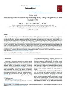
main variable of interest - the monthly number of international tourists from the top 12 origin countries over the period January 1991 to December 2010. Inbound tourist arrivals is deemed a better demand proxy than tourism receipts since arrival data are more accurately measured and monitored through airlines/shipping manifests and related documents, while receipts are often estimated through sample surveys. An overwhelming majority of empirical forecasting studies surveyed in the literature use arrival data to represent tourism demand (Lim, 1997). The ranking of countries based on the 2010 data are presented in Table 1. It shows that the top three countries – South Korea, USA, and Japan - captured almost half (48.28 %) of the Philippines’ total international tourism market. Closer scrutiny of the table will further reveal that about one in five tourists who arrived in 2010 was a Korean, while about one in every four arrivals was either an American or Japanese. Doubledigit rate of growth was registered by most of the 12 countries relative to their respective figures during the crisis year 2009. Curiously, short-haul tourism source countries South Korea, Taiwan, Singapore, Malaysia, Japan and Hong Kong turned in double-digit growth figures with rates of 48.74 %, 39.29 %, 23.17 %, 16.04 %, 10.39 % and 10.39 % respectively. Furthermore, it is also interesting to note that all long-haul countries in the top twelve, registered single-digit growth rates, while other countries outside the top 12 recorded a disappointing drop of 16.82 % from their collective total in 2009. Statistical Properties of MontHly Tourist Arrivals Presented in Figure 2 are the line graphs of the different arrival series over the sample period January 1991 to December 2010. The graphs depict the somewhat erratic movements of the primary demand variable of the study. One may surmise that these variables are highly sensitive to a host of factors, that to develop structural models

FORECASTING INTERNATIONAL DEMAND FOR PHILIPPINE TOURISM

RUFINO, C.C.

63

Table 1 Top 12 Origin Countries of Philippine International Tourism 2009-2010 Rank in 2010

Visitors from

Arrivals in 2010

Market Share

Arrivals in 2009

Growth Rate

1

Korea

740,622

21.04%

497,936

48.74%

2

USA

600,165

17.05%

582,537

3.03%

3

Japan

358,744

10.19%

324,980

10.39%

4

China

187,446

5.32%

155,019

20.92%

5

Australia

147,469

4.19%

132,330

4.08%

6

Taiwan

142,455

4.05%

102,274

39.29%

7

Hong Kong

133,746

3.80%

122,786

10.39%

8

Singapore

121,083

3.44%

98,305

23.17%

9

Canada

106,345

3.02%

99,012

7.41%

10

United Kingdom

96,925

2.75%

91,009

6.50%

11

Malaysia

79,694

2.26%

68,679

16.04%

12

Germany

58,725

1.67%

55,912

5.03%

Other Countries

52,066

62,597

-16.82%

(Source:www.tourism.gov.ph)

for them in aid of forecasting may prove to be a formidable task. Most of the series display regular upward and downward spikes during specific months of each year. This is specially so for Australia, Canada, United Kingdom and United States. The same tendency is recognizable but less pronounced in the graphs of other countries. Various parts of the series also exhibit the tendency of steadily up-trending behavior after encountering a local trough in the year 2002. Although this is not a general characteristic for all series, the appearance of this inflection point can be observed in about half of the cases. Interestingly, most of the series demonstrate tendencies to spike abruptly or shift vertically during or after certain periods. To an inexperienced observer, extracting meaning from the mechanisms that brought

about the observed visitor arrivals across time may seem to be extremely difficult. However, for a seasoned analyst, some indications are recognizable about their statistical regularity. Hopefully, these can be extracted to assist in forecasting. On the other hand, a causal model builder may have different ideas about the appearance of the observed peaks and troughs in the series. In this study, we take the point of view of an a-theoretic (non-causal) analyst who wants to dig up predictive information from historical time series to gain insights on the data-generating process underlying each series without having to lean on any rigid theoretical structure (see Song and Li (2008) and Witt and Witt (1995) for detailed reviews of tourism forecasting approaches). Furthermore, it is crucial to accommodate in the modeling process

64


calendar variations and unexpected events (e.g. travel advisories, epidemics, natural calamities, terrorist attacks, changes in government policies, among others) in predicting the potential impacts of these one-off occurrences on tourism demand. Our choice of the non-structural modeling strategy is motivated by the growing body of evidence in the literature on the non-suitability of static econometric models in forecasting future magnitudes of the dependent variable (Witt & Witt, 1995; Li, Song & Witt 2005, Song & Li, 2008). Their comparative advantage, however, is in estimating coefficients of economic relationships useful in policy formulation such as elasticities, multipliers, marginal propensities and other decision-making parameters. These structural models, when used for forecasting, will require forecasts or policy values of the explanatory variables. At times, such values may only be extrapolated with substantial error. Furthermore, most econometric models also suffer from the “Lucas Critique” or the model’s inability to predict the future when the future is anchored on a structural change brought about by the adoption of a new policy (Lucas, 1976). Isolating the Secular Trend To make a systematic attempt in figuring out the unknown data-generating mechanism for each visitor arrival series, we have to assume that each of the observed value of the series is a composite of four distinct components: (1) the secular trend; (2) the seasonality; (3) the cyclical oscillation; and (4) the irregular variation or the background noise. The secular trend is the general direction the series is taking. Isolating this component offers clues on the long-term trajectory of the observed series. The seasonality of the series pertains to its recurring behavior during specific times, year after year. The cyclical component is that particular part of any time series linked to the general economic and business cycles of

VOL. 21 NO. 1

growth and decline, and is longer in periodicity than one full seasonal movement. Finally, the irregular component is that portion which has no assignable causes, and is usually assumed as a random noise component. In visualizing the secular trend of an economic series, macroeconomists typically resort to certain smoothing techniques to trim away smaller fluctuations in the series in order to highlight the straightforward direction of the variable over time. Most analysts use some form of mechanical moving average procedures. Others just outline a free-hand straight or curved line in forming the secular trend. The Hodrick-Prescott filter is considered by many to be the current state of the art tool (Hodrick & Prescott, 1997) in isolating the secular trend. The Hodrick-Prescott trend (HP) st is determined by minimizing the variance of the time series yt around this trend. Mathematically, the objective is to choose st such that the following expression is minimized: T

∑ ( yt − st )2 + l t =1

T

∑ {( s t =2

t +1

− st ) − ( st − st −1 )}

2

Where l is an arbitrary constant, which represent the penalty of trend fluctuations, expressed by the second-order differences. The greater l is, the smoother the trend series st becomes. Hodrick and Prescott (1997) suggested a penalty of l = 14400 for monthly series, which we adopt in this study. The HP trend st for each of the monthly visitor arrival series is computed through the Eviews 5.0 software. The resulting secular trend series are graphically presented in Figure 3 below. The graphs of the HP secular trends of the series confirm our initial observation from the line graphs of the original series in Figure 2 - most of the countries appear to form turning points in their graphs sometime in 2002 and subsequently achieved all-time high visitor arrivals. Using the graphs of HP trends in Figure 3, clearer insights can be drawn regarding the general direction of the demand of each of the 12 countries for Philippine international tourism.


From the different HP graphs, it is clear that based on the nationalities of visitors, all countries are generally on the uptrend. The steepest ascent is posted by China, Australia, Singapore, United Kingdom and Malaysia which have been on an exponentially upward trend since the later part of 2002. South Korea also displayed remarkable performance, as its secular trend registered steep gradient, and is seen to be on this mode longer than the other countries. South Korea’s fairly linear up trending behavior started sometime in the second half of 1998. Seasonality Analysis Seasonality of tourism demand is a central theme in tourism literature which carries wideranging implications in policymaking and practical tourism management (Koenig & Bischoff, 2003). Although the importance of seasonality in tourism research is well recognized, this phenomenon is, at the same time, one of the

RUFINO, C.C.

least understood (Hingham & Hirsch, 2002). This intra-year regularity of the observed time series, in the context of tourism demand analysis, is caused by a host of factors. Among these factors, weather is the most dominant. In a country such as the Philippines whose tourism attractions are mostly “climate dependent” outdoor recreation facilities (e.g. beaches, resorts, countryside attractions, etc.), the extent of tourism activities is wholly dependent on weather conditions or climate. Destinations relying on such outdoor facilities are more likely to experience pronounced seasonality in the conduct of their tourism businesses. Our initial observation of the regularly occurring spikes and bottoms for most graphs in Figure 1 may be explained by the phenomenon of seasonality. This observation is not surprising since tourists from affluent countries like Australia, Canada, United Kingdom and United States of America mostly visit the Philippines for holiday merry-making, rest and recreation during specific months of any year.

Table 2 Seasonality Testing of International Tourist Arrivals Source Country

Moving Seasonality

Stable Seasonality

K-W Seasonality

F-Value

p-value

F-Value

p-value

Chi-Square

p-value

Australia

1.186

0.2951

87.086

0.0000

102.158

0.0000

Canada

1.352

0.1903

104.513

0.0000

141.069

0.0000

China

1.684

0.0703

2.425

0.0820

25.990

0.0610

Germany

1.865

0.0388

48.047

0.0000

140.014

0.0000

Hong Kong

3.214

0.0030

6.6639

0.0000

57.643

0.0000

Japan

1.279

0.2320

27.798

0.0000

112.598

0.0000

Korea

5.607

0.0000

27.592

0.0000

110.068

0.0000

Malaysia

2.058

0.0201

9.178

0.0000

53.933

0.0000

Singapore

2.494

0.0042

10.316

0.0000

64.293

0.0000

Taiwan

3.215

0.0030

4.249

0.0000

47.572

0.0018

United Kingdom

1.857

0.0400

18.023

0.0000

134.498

0.0000

United States

1.014

0.4415

48.638

0.0000

138.082

0.0000

(Source:www.tourism.gov.ph)

65

66


Formal statistical tests for both stable and moving form of seasonality were done to empirically verify the presence of seasonality in the twelve tourism demand series. Stable seasonality implies the presence of regularly occurring peak and lean periods during specific months of any year. Moving seasonality, on the other hand, is a form of seasonality when intrayear shifting of peak and lean months occur over time. Table 2 summarizes the results of the tests for both the moving and stable seasonality of the visitor arrival series via the seasonality diagnostics (F-tests and Kruskall-Wallis test) feature of Census X12 routine of Eviews 5.0. Conclusions drawn from the results of the tests confirm our initial suspicion that pronounced seasonality of tourism arrivals exists. Under the null hypothesis of no stable seasonality, statistically significant results are noted for all countries. This means that stable seasonality exists for the visitor arrival series of all countries. Absence of moving seasonality at the one percent significance level is noted in eight countries - Australia, Canada, China, Germany, Japan, Malaysia, UK, and USA. For the other four countries, moving seasonality is present. The foregoing tests give us the indication that seasonality will have to be considered in the modeling process. Modeling Framework The ARIMA model-based approach will be used in depicting the monthly visitor arrival time series for each of the top twelve tourists sending countries to the Philippines. It is postulated in this study that the observed visitor time series for each country is generated by a stochastic process driven by a host of deterministic factors and a Seasonal Auto Regressive Integrated Moving Average (SARIMA) type noise element. These factors, known as calendar effects are mainly classified into two categories: trading day (TD) effects caused by the different distribution of weekdays in different months and captured by the number

VOL. 21 NO. 1

of trading days of the month and the Easter effect (EE), which captures the moving dates of Easter in different years. The other deterministic factors are called outliers – events which happen on certain months capable of shifting levels or directions of the time series. Outliers are further categorized into three different types – Additive Outliers (AO), Transitory Change outliers (TC) and Level Shift (LS) outliers. AO outliers are events that cause one-time spikes in the series; TC outliers create transitory changes, while Level shifters are shocks with permanent effects. Symbolically, if Yit is the number of tourist arrivals from the ith tourist sending country to the Philippines during month t and Dsjit is a dummy variable that indicates the position of the sth event of the category jth outlier (i.e. AO, TC and LS, for the ith country during month t and TDt is the number of trading days in month t and DEEt = 1 if Easter occurs during month t, zero otherwise), the model can be specified as follows: Yit = j i + y

TDt TDt + y

EEt DEEt +

LS

nj

∑ ∑y

j = AO s =1

sjit

D(1.1) sjit + X it

for the ith country (i=1 for South Korea, i=2 for U.S, …, i=12 for Malaysia) and t = January 1991, …, December 2010. The parameter y sjit is the effect of the sth event of the jth outlier type on the arrivals from the ith country during time t and n j = number of j type outlier. The variable X it is a stochastic noise element (random error) that follows an ARIMA( p, d , q )( P, D, Q )12 process for each country over time. Algebraically, the noise X it is represented in lag polynomial form as: f p ( L)Φ P ( L)d ( L) X it = qq ( L)ΘQ ( L)eit (1.2) Where eit is a white noise innovation (i.e. i.i.d. with mean zero and constant variance), f p ( L), Φ P ( L), qq ( L) and ΘQ ( L) are finite lag polynomials in L (lag notation with the property Ln yt = yt − n ). The first two contain respectively the p stationary regular AR roots and the P seasonal AR roots of X it , the last two contain the


q invertible regular MA roots and Q invertible seasonal MA roots of X it respectively. These lag polynomials are specified as: f p ( L) = 1 − f 1 L − f 2 L2 − ... − f p Lp autoregressive lag polynomial

→ regular

Φ P ( L) = 1 − Φ1 Ls − Φ 2 L2 s − ... − Φ P LPs → seasonal autoregressive lag polynomial qq ( L) = 1 + q1 L + q2 L2 + ... + qq Lq → moving average lag polynomial

regular

Φ Q ( L) = 1 + Φ1 Ls + Φ 2 L2 s + ... + Φ Q LQs → seasonal moving average The lag polynomial d ( L) = (1 − L) d (1 − Ls ) D = ∇ d ∇ sD contains the d non-seasonal unit roots and the D seasonal unit roots of X t . This transformation converts the series into stationary stochastic process. The parameter j i represents the intercept for the ith country. Summary of the Estimation and Inference Procedure The standard procedure implemented by well known softwares for signal extraction in univariate time series (e.g. the reg-ARIMA component of Census X-12 and the TRAMO component of TRAMO-SEATS) is adopted in this study to establish the estimated models (1.1) and (1.2) for the stochastic noise of each tourist arrivals series. The procedure assumes initially that the background noise for each series follows the parsimonious default model known as the Airline Model ( ARIMA(0,1,1)(0,1,1)12 ). The Airline Model is well suited for a large number of real-world time series (Box, G. & Jenkins, G, 1970) and has become a benchmark model in modern time series analysis. The Airline Model1∗ is initially applied to the series and then pre-tested for the log-level specification using the Schwarz Information Criterion (SIC) as basis of choice. Once the

RUFINO, C.C.

67

decision to use either the level or log transformed version of the series is reached, regressions are then run for the residuals of the default model to test for Trading Day (TD) and Easter (EE) Effects, after which an iterative procedure is implemented to identify the various outliers. This procedure iterates between the following two stages - (1) outlier detection and correction and (2) identification of an improved model. To maintain model’s parsimony, model identification is confined within the following narrow ranges: 0 ≤ p, q ≤ 3 and 0 ≤ P, Q ≤ 2 for the regular/ seasonal autoregressive/moving average orders, and 0 ≤ d ≤ 2 , 0 ≤ D ≤ 1 for the number of regular and seasonal unit roots respectively. Pre-testing for the presence of deterministic mean mi of X it is also embedded in the procedure, in which case, the X it in (1.1) and (1.2) is to be replaced by its de-meaned value xit = X it − mi . Aside from testing the statistical adequacy of the parameters, the following diagnostic procedures will be implemented to handle the models adequacy: the Ljung-Box (Q) test for residual autocorrelation, the Jarque-Bera (JB) test for normality of residuals, the SK and Kur t-tests for skewness and kurtosis of the residuals, the Pierce (QS) test of residual seasonality, the McLeod and Li (Q2) test of residual linearity and the Runs t-test for residuals randomness. The Exact Maximum Likelihood Estimation (EML) procedure via the Kalman Filter is used in parameter estimation and inference. The HannanRissanen (H-R) Method is used to get starting values for likelihood evaluation. Once the best model for each arrival series is established, a full year (12 months) ex-ante forecasts will be generated. The TRAMO routine in TSW (TRAMOSEATS for Windows) Beta Version 1.04 Rev. 177 (Caporello & Maravall, 2010) is used to implement the estimation, inference, diagnostics and forecasting procedures. This software is considered as at the leading edge in signal extraction via ARIMA Model Based approach currently in use by data agencies of major OECD countries. This study exploits the capability of

68


VOL. 21 NO. 1

Table 3 Calendar Effects and Outliers Detected for Each Arrival Series Calendar Effects Monthly Arrivals From

Outliers (Number of Events)

Trading Day Effect (TD)

Easter Effect (EE)

Additive Outliers (AO)

Transitory Changers (TC)

Level Shifters (LS)

USA

Insignificant

Insignificant

3

5

0

Japan

Insignificant

Insignificant

2

1

1

Korea

Insignificant

Insignificant

3

3

3

Hong Kong

Insignificant

Insignificant

1

0

0

Taiwan

Insignificant

Insignificant

2

2

3

Australia

Insignificant

Insignificant

1

0

0

Canada

Insignificant

Insignificant

1

1

1

Singapore

Insignificant

Insignificant

1

5

0

UK

Insignificant

Insignificant

4

1

3

Germany

Insignificant

Insignificant

1

2

0

China

Insignificant

Insignificant

1

0

2

Malaysia

Insignificant

Insignificant

3

1

1

the software to do modeling in automatic mode, handling multiple time series at a time, thereby cutting modeling time considerably. The challenge in using the software lies in the preparation and fine-tuning of the necessary modeling instructions and inputs consistent with the modeling framework being used. Results of the Modeling Process Successive runs of the TSW software in production mode produced a sequence of valuable information on the data generating mechanism which underlie the different tourism demand series. These pieces of information are amply summarized and presented in a number of matrices and statistical tables pre-formatted

by the software. When this information was collated the deterministic Calendar Effects and influential outliers as well as the final SARIMAnoise models for the different tourism demand series emerged and are presented in Table 3 and Table 4 respectively below. Tabulated summary of the various diagnostics of models’ desirability are exhibited in Table 5. Summarized in Table 3 are the results of modeling the deterministic components of model (1.1). The table reveals the insignificance of the calendar effects (trading day and Easter) for all of the countries. Also presented is the frequency distribution of the various outlier categories detected by the TRAMO program for each country. Maximum number of the additive outliers (AO) is 4, detected for the United Kingdom; the most number of transitory changers (TC) were


RUFINO, C.C.

69

Table 4 Final SARIMA Noise Models for Each Arrival Series Monthly Arrivals From

ARIMA Noise Model

In Levels or Log Transformed

With Mean or Without Mean

USA

ARIMA(0,1,1)(0,1,1)12

In Levels

Without Mean

Japan

ARIMA(0,1,1)(0,1,1)12

In Levels

Without Mean

Korea

ARIMA(3,1,1)(0,1,1)12

Log Transformed

Without Mean

Hong Kong

ARIMA(0,1, 2)(0,1,1)12

Log Transformed

Without Mean

Taiwan

ARIMA(0,1,1)(0,1,1)12

Log Transformed

Without Mean

Australia

ARIMA(0,1,1)(0,1,1)12

Log Transformed

Without Mean

Canada

ARIMA(0,1, 3)(0,1,1)12

Log Transformed

Without Mean

Singapore

ARIMA(0,1,1)(0,1,1)12

In Levels

Without Mean

UK

ARIMA(0,1,1)(0,1,1)12

Log Transformed

Without Mean

Germany

ARIMA(0,1,1)(1,1,1)12

Log Transformed

Without Mean

China

ARIMA(0,1,1)(0, 0, 0)12

Log Transformed

Without Mean

Malaysia

ARIMA(0,1,1)(0,1,1)12

Log Transformed

Without Mean

noted for USA and Singapore at 5 events each, and maximum numbers of level shift (LS) outliers were posted by South Korea, Taiwan and UK at 3 apiece. The countries which have the least number of outliers are Hong Kong and Australia at only 1 significant outlier out of 240 month observations. South Korea has the most number of total outliers with 9. Summary statistics of the most adequate noise model for each arrival series are exhibited in Table 4. It shows that the majority of the series required the logarithmic transformation prior to noise modeling. Only USA, Japan and Singapore arrival series were modeled in level. The TRAMO procedure deemed all series, except China required the ∇∇12 transformation for the original series to be converted stationary. The absence of

the seasonal unit roots for China supported the insignificant seasonality test results shown in Table 2 for this country. Monthly arrivals from USA, Japan and Singapore follow basically identical noise model exemplified by the benchmark Airline Model in logarithmic transformed form. Unique stochastic processes underlie South Korea, Hong Kong, Canada and China. The results of the various diagnostic tests are presented in Table 5. The statistics Q refers to the Ljung-Box test for residual autocorrelation, which in our case follows a c 2 distribution with approximately 22 degrees of freedom. JB is the Jarque-Bera test for normality of the residuals having c 2 distribution with 2 degrees of freedom; SK and Kur are t-test for skewness and kurtosis respectively of the residual series. QS is the

1

1

0

0

0

0

0

1

0

0

0

0

USA

JAPAN

KOREA

HONG KONG

TAIWAN

AUSTRALIA

CANADA

SINGAPORE

UK

GERMANY

CHINA

MALAYSIA

SERIES

Level(1) or Log(0)

0

0

0

0

0

0

0

0

0

0

0

0

Mean

With or W/o

0

0

0

0

0

0

0

0

0

3

0

0

p

1

1

1

1

1

1

1

1

1

1

1

1

d

1

1

1

1

1

3

1

1

1

1

1

1

q

0

0

0

0

0

0

0

0

0

0

0

0

P

1

0

1

1

1

1

1

1

1

1

1

1

D

SARIMA Model

1

0

1

1

1

1

1

1

1

1

1

1

Q

0.1376

0.2410

0.1156

0.0990

461.38

0.0973

0.0915

0.1764

0.1986

0.1216

2178.6

2265.9

SE of Residuals

-3.8302

-2.7709

-4.1985

-4.4119

12.4431

-4.5048

-4.7236

-3.2953

-3.0588

-3.9622

15.4890

15.6454

SIC

Table 5 Summary of the Diagnostics Results of the Final SARIMA Noise Models

19.69

26.83

21.25

24.57

16.94

21.73

25.17

26.54

21.43

35.16

34.38

29.44

QStat

0.728

0.089

0.484

5.350

5.310

3.070

7.680

14.700

1.050

0.195

1.650

0.260

JB-test

0.486

-0.200

-0.240

1.930

0.452

-1.750

-0.210

-2.330

-0.790

0.433

1.260

-0.060

SK t-test

0.701

0.218

0.652

1.280

2.260

-0.120

2.760

3.050

0.653

-0.090

0.277

-0.510

KUR t-test

QS

1.540

1.060

1.310

0.000

0.123

0.376

0.079

0.000

0.000

0.269

0.969

0.000

Residual Tests

28.11

48.73

30.41

20.63

20.26

26.72

32.80

25.16

41.87

32.14

38.08

35.13

Q2

0.673

0.261

-0.670

-0.950

-0.810

-1.750

-1.470

-0.950

-1.760

0.271

-0.130

-0.950

RUNS t-test

70 DLSU BUSINESS & ECONOMICS REVIEW VOL. 21 NO. 1

Total 2011

December

November

October

September

August

July

June

May

April

March

February

January

Monthly Arrival Forecast in 2011

368,167

32,752 (2,178) 30,586 (2,434) 33,375 (2,666) 30,091 (2,879) 27,282 (3,077) 26,745 (3,264) 30,673 (3,440) 36,631 (3,608) 32,760 (3,768) 28,754 (3,921) 27,787 (4,069) 30,731 (4,212)

57,387 (2,303) 48,812 (2,480) 57,527 (2,645) 55,266 (2,802) 56,284 (2,947) 53,898 (3,087) 52,186 (3,221) 41,032 (3,350) 38,808 (3,474) 49,009 (3,593) 47,818 (3,709) 61,627 (3,821)

619,654

Japan

USA

938,885

95,635 (11,230) 73,039 (9,914) 68,760 (9,931) 64,314 (9,457) 70,960 (10,697) 68,957 (10,744) 88,065 (14,260) 82,465 (13,830) 66,179 (11,407) 70,408 (12,459) 86,919 (15,888) 103,184 (19,351)

Korea

10,200 (2,406) 12,531 (3,094) 10,453 (2,641) 11,016 (2,846) 9,357 (2,470) 10,141 (2,732) 11,259 (3,093) 11,480 (3,215) 9,410 (2,684) 10,236 (2,972) 9,202 (2,718) 10,833 (3,254) 126,118

Hong Kong

166,698

13,295 (2,364) 16,709 (3,447) 12,216 (2,779) 11,754 (2,912) 12,615 (3,368) 14,410 (4,110) 17,761 (5,373) 17,264 (5,509) 13,659 (4,576) 13,240 (4,639) 11,805 (4,311) 11,970 (4,544)

Taiwan

164,637

13,790 (1,265) 11,241 (1,112) 14,602 (1,544) 13,643 (1,529) 12,686 (1,498) 11,919 (1,476) 11,353 (1,468) 10,709 (1,441) 12,333 (1,723) 13,285 (1,921) 14,226 (2,124) 25,008 (3,850)

Australia

114,868

12,504 (1,290) 8,606 (929) 11,040 (1,294) 9,517 (1,151) 9,823 (1,203) 6,209 (776) 8,733 (1,114) 6,318 (821) 6,325 (837) 8,283 (1,116) 10,339 (1,417) 17,171 (2,393)

Canada

126,229

9,469 (511) 9,983 (546) 10,858 (578) 10,262 (609) 10,607 (639) 10,680 (667) 10,175 (694) 10,511 (720) 10,471 (745) 10,414 (769) 12,050 (793) 10,749 (854)

Singapore

100,721

8,463 (877) 7,079 (754) 10,969 (1,201) 8,810 (990) 8,094 (932) 6,592 (777) 9,122 (1,099) 7,175 (883) 6,051 (760) 7,534 (966) 8,785 (1,147) 12,047 (1,602)

UK

59,486

5976 (694) 5267 (652) 6,944 (909) 4,635 (638) 3,994 (576) 3,275 (492) 5,075 (793) 4,500 (729) 3,148 (527) 4,374 (756) 5291 (943) 7,007 (1,285

Germany

368,167

32,752 (2,178) 30,586 (2,434) 33,375 (2,666) 30,091 (2,879) 27,282 (3,077) 26,745 (3,264) 30,673 (3,440) 36,631 (3,608) 32,760 (3,768) 28754 (3,921) 27,787 (4,069) 30,731 (4,212)

China

Table 6 Full Calendar Year 2011 Ex-Ante Forecasts for Monthly Visitor Arrivals Generated by the Models (Std Errors in Parentheses)

92,578

6,700 (954) 7,218 (1,077) 8,155 (1,299) 6,888 (1,164) 7,701 (1,371) 7,567 (1,413) 7625 (1,487) 7,954 (1,615) 7,682 (1,616) 7,642 (1,667) 9,191 (2,072) 8,255 (1,919)

Malaysia

FORECASTING INTERNATIONAL DEMAND FOR PHILIPPINE TOURISM RUFINO, C.C. 71

0

2000

4000

6000

8000

10000

12000

14000

0

4000

8000

12000

16000

20000

24000

0

4000

8000

12000

16000

20000

24000

92

92

92

94

94

94

98

98

98

02

04

02

04

02

04

S INGA PORE

00

HONGK ONG

00

A US T RA LIA

00

06

06

06

08

08

08

10

10

10

02

02

02

04

04

04

06

06

06

08

08

08

10

10

10

0 T A IW AN

02

04

06

08

08

10

10

1000

8000

10000

12000

0

0

92

94

96

98

00

U_K

02

KORE A

04

06

08

10

10000

20000

30000

40000

50000

60000

70000

0

1000

2000

10000

3000

20000

4000

30000

5000

6000

40000

02

06

50000

60000

00

04

7000

CHINA

00

8000

98

98

70000

96

96

9000

94

94

80000

92

92

2000

3000

4000

5000

6000

7000

8000

9000

90000

2000

00

JAPAN

00

CA NA DA

00

4000

98

98

98

5000

96

96

96

10000

94

94

94

6000

92

92

92

0

4000

8000

12000

16000

20000

24000

15000

20000

25000

30000

10000

15000

20000

25000

30000

35000

40000

45000

0

4000

8000

12000

16000

20000

92

92

92

94

94

94

96

96

96

98

98

98

00

02

04

02

04

02 US A

00

04

MA LA Y S IA

00

GE RMA NY

06

06

06

08

08

08

10

10

10


Figure 1. Monthly Visitor Arrivals from t he Top 12 Origin Countries Jan 1991 to December 2010

96

96

96

72 VOL. 21 NO. 1

0

2000

4000

6000

8000

10000

12000

4000

6000

8000

10000

12000

14000

2000

4000

6000

8000

10000

12000

14000

92

92

92

94

94

94

96

96

96

00

02

04

00

02

04

00

02

04

08

08

08

10

10

10

0

4000

8000

12000

16000

20000

15000

20000

25000

30000

35000

92

92

92

94

94

94

96

96

96

98

98

98

00

02

04

02

04

02

04

T A IW AN_HP

00

J A PA N_HP

00

CA NA DA _HP

06

06

06

08

08

08

10

10

10

98

98

00

02

04

06

08

10

10

2000

3000

4000

5000

6000

7000

8000

9000

0

92

94

96

98

02 UK _HP

00

04

KORE A_HP

06

08

10

10000

20000

30000

40000

50000

0

1000

2000

10000

3000

20000

5000 4000

04

08

30000

02

06

40000

50000

00

CHINA _HP

6000

96

96

7000

94

94

60000

92

92

2000

2500

3000

3500

4000

4500

5000

5500

70000

0

4000

8000

12000

16000

92

92

92

94

94

94

96

96

96

00

02

04

00

02

04

98

02 US A_HP

00

04

MA LA YSIA_HP

98

GE RMANY_HP

98

Figure 2. Hodrick-Prescott Secular Trends of Monthly Tourist Arrivals from Top 12 Origin Countries January 1991 to Dec 2010

06

06

06

SINGA PORE _HP

98

HONGKONG_HP

98

AUST RA LIA_HP

98

1000

2000

3000

4000

5000

6000

7000

8000

9000

10000

06

06

06

08

08

08

10

10

10

FORECASTING INTERNATIONAL DEMAND FOR PHILIPPINE TOURISM RUFINO, C.C. 73

74


modified Pierce test for for seasonality of the residuals which is c 2 with 2 degrees of freedom, Q2 represents the Mcleod-Li test of residual linearity ( c 2 with 24 degrees of freedom) and finally, Runs is a t-test for the randomness in the algebraic signs of the residuals. Very few of the series failed some of the diagnostics at the 5% level of significance but all pass the most relevant Ljung-Box test of residual autocorrelation signifying the success of the differencing transformation in converting the series into stationary stochastic processes. Together with the different deterministic effects, the different forecasting models for each arrival series were estimated for use in the generation of ex-ante forecasts for the full year monthly visitor arrivals (January 2011 to December 2011) from each of the 12 top sources of international tourists to the Philippines. Presented in Table 6 are the monthly visitor arrivals forecasts (with forecast standard errors in parenthesis) generated by the models for January 2011 to December 2011 From these forecasts, it is estimated that for the year 2011, international tourist arrivals will reach an all-time high of 4,057,760 visitors, about 80 % of which will come from the top 12 traditional sources. South Koreans are again expected to dominate arrivals with a whole year estimate of 938,885 followed by Americans with 619,654 and Japanese with 368,167 visitors. Concluding Remarks Accurate prediction of the number of international tourists who will visit the country is an absolute requisite for effective tourism planning. For a well-endowed country as the Philippines, which has all the potentials to become a force to reckon with in international tourism, effective planning is sorely needed. The government, on its part, is not remiss in formulating tourism plans and strategies over the years, yet the country has been lagging behind neighboring countries in attracting international visitors. In most of the 2000 decade, Vietnam

VOL. 21 NO. 1

overshadowed the Philippines in attracting foreign tourists, despite coming from decades of isolation and devastating wars. Indonesia, an archipelago more fragmented than the Philippines, had almost three times as many international visitors. Even the tiny city-state of Singapore hosted more than four times as many international visitors than the Philippines in any given year. Malaysia and Thailand are the top two most favored destinations of foreign tourists in the South East Asia region. In the current decade, these two individually enjoy at least five- folds numerical superiority per year over the Philippines in visitor arrivals. A plethora of reasons may be put forward by analysts of various persuasions as to why the country is languishing in mediocre performance in attracting foreign visitors. One of these reasons maybe that of ill-conceived planning, or to be more specific, meager anticipation of the demand for the country’s international tourism. Estimates of the expected future demand constitute a very important element in all planning activities. In the context of tourism, accurate forecasts of tourism demand are essential for efficient planning by tourism-related businesses, particularly given the perishable nature of the tourism product and the highly seasonal nature of its occurrence (Higham & Hinch, 2002). This study is an attempt to develop and operationalize empirical forecasting models for the monthly number of tourists coming to the Philippines from the top source countries. Employing a framework that takes into account possible influential events that impact on the level and direction of arrival series, together with a reliable procedure of modeling background noise, the study is able to establish forecasting models that passed all conventional selection criteria. These models are used in predicting future visitor arrivals from each of the 12 countries for a fullyear planning horizon. The proponent is hopeful that government and private tourism planners will adopt the modeling framework and the procedures used in the study in designing geographically segmented short- to medium-term action plans and effective marketing


strategies to energize Philippine tourism. Much has been said and written about the massive economic benefits a country can derive from international tourism, and the Philippines has yet to capitalize on its enormous natural endowments and comparative advantage to cash-in on the unprecedented global growth of this industry. Note 1

This model resulted from the use of ARIMA methodology to Airline Passengers data set by Box & Jenkins (1970) and has become the standard seasonal ARIMA model in the literature.

∗

References Box, G.E.P., & Jenkins, G. (1970). Time series analysis, forecasting and control. San Francisco: Holden Day Caporello, G., & Maravall, A. (2010). TSW (TRAMO-SEATS for Windows) Beta Version 1.04 Rev. 177 [computer software]. Spain: Bank of Spain. Egan, D., & Nield, K. (2003). The economic impact of tourism – A critical review. Journal of Hospitality and Tourism Management, 10(2), 170-177 Higham, J., & Hinch, T.D. (2002). Tourism, sports and seasons: the challenges and potential of overcoming seasonality in the sports and tourism sectors. Tourism Management, 23(2), 175-185.

RUFINO, C.C.

75

Hodrick, R., & Prescott, E. (1997). Post-war business cycles: an empirical investigation. Journal of Money, Credit and Banking, 29(1), 1-16. Koenig, N., & Bischoff, E. (2003). Seasonality of tourism in Wales: A comparative analysis. Tourism Economics, 9(3), 229-254. Li, G., Song, H., & Witt, S.F. (2005). Recent developments in econometric modeling and forecasting. Journal of Travel Research, 44(1), 82-99. Lim, C. (1997). Review of international tourism demand models. Annals of Tourism Research, 24(4), 835-849. Lucas, R. (1976). Econometric policy evaluation: A critique. In K. Brunner (Ed.), The Phillips Curve and Labor Markets, Carnegie-Rochester Conference Series on Public Policy, (1), 1946 Sinclair, M.T. (1998). Tourism and economic development: A survey. The Journal of Development Studies, 34(5), 1-51. Song, H., & Li, H. (2008). Tourism demand modeling and forecasting – A review of recent research. Tourism Management, 29(2), 203220. World Tourism Organization [UNWTO]. UNWTO World Tourism Barometer, January 2011 release UNWTO Tourism Highlights, 2010 Print Edition Witt, S.F., & Witt, C.A. (1995). Forecasting tourism demand: A review of empirical research. International Journal of Forecasting, 11(3), 447-475.