Jul 3, 2015 - line inflation in the Polish economy over the period 2011-2014 employing ... seasonal dummies and at lags of each variable. On the one hand, ...
Forecasting the Polish in�ation using Bayesian VAR models with seasonality Damian Stelmasiak, Grzegorz Szafra«ski July 3, 2015
Abstract
Bayesian VAR models o�er practical solutions to the parameter proliferation concerns as they explicitly allow to incorporate a priori information on seasonality and persistence in multivariate price dynamics. We investigate into the alternative prior speci�cations in the case of time series with clear seasonal pattern. Empirically, we forecast the monthly headline in�ation in the Polish economy over the period 2011-2014 employing two popular BVAR frameworks. To evaluate forecast performance we use the pseudo real-time vintages of timely information from consumer and �nancial markets. We compare di�erent models in terms of, both, point and density forecast performance. Using formal testing procedure we provide the evidence of superiority of density forecasts from the steady-state BVAR speci�cations.
Keywords: Bayesian VAR, forecasting in�ation, seasonality, steady-state prior, real-time forecasting, logarithmic score, Continuous Ranked Probability Score JEL Classi�cation:
C32, C53, E31, E37
1
1
Introduction
Consumer prices are continuously under in�uence of various price factors including shocks from many markets (food, energy, commodities, and currency, to name the most important). Many of these price indicators are observed within a current month or a quarter when the forecast is prepared. It is a common practice to take their persistent role into account by using a multivariate, dynamic framework like a vector autoregression (VAR) model. We argue that using quarterly or monthly data in a regular short-term forecasting requires a careful treatment of their seasonality. A prior knowledge on time-series properties of the data brings an important input into both point and interval predictions if one deals properly with the curse of dimensionality (see Ba«bura et al., 2010). Since Sims (1980) introduced VAR models into macroeconomics it took many years to develop the framework into a standard tool for a short-term forecasting. The main drawback of empirical VARs relies in the increased number of parameters to be estimated. The excess parameter uncertainty introduces serious limitations in producing reliable out-of-sample density forecasts. In a VAR framework with seasonal time series these limitations become binding very fast. For example, at monthly data frequency a �ve-variate VAR model of lag order 12 requires as many as 360 parameters to be estimated including parameters at seasonal dummies and at lags of each variable. On the one hand, potentially rich parametrization of seasonal VARs poses over-�tting concerns in sample and increases the risk of poor out-of-sample forecasting performance. On the other hand, severe consequences could a�ect the forecast mean and variance after a big shock in any of important but omitted variables. To make VAR model operational, the researchers introduce restrictions on parameter space in a Bayesian framework by means of prior distributions (priors). Conventionally, the starting point is a Bayesian VAR (BVAR) model in a reduced-form with a system of priors known as Minnesota-type priors. These ideas come from seminal paper of Litterman (1979) and are further developed in Doan et al. (1984) and Litterman (1986). The Minnesota priors on parameters at consecutive lags of dependent variables take the form of independent normal distributions with variances being combinations of a relatively small number of hyperparameters. The role of these hyperparameters consists of shrinking the dynamics of multivariate time series around a priori beliefs on the time-series properties of the data. The shrinkage for each of the variables is usually centred towards simple univariate stationary autoregressive (AR) or unit-root random walk (RW) processes. Optimal values of the Minnesota hyperparameters in BVAR models are commonly set by simple rules of thumbs or by some out-of-sample forecasting criteria (e.g. RMSFE in a training period). The most popular in this conventional approach are the following heuristic rules: harder shrinkage of VAR parameters towards zero for longer lags, scaling variances of parameters at other variables by standard deviations of errors from AR model and decaying them faster towards zero than for their own lags. Following Litterman (1979) seminal paper 2
these priors are often combined with an assumption of a diagonal error covariance matrix. Many other enhancements and re�nements are proposed to improve the forecasting performance of BVARs. The proper treatment of initial observations and inexact di�erencing, both using Theil mixed estimation approach, are the most popular between them. Kadiyala and Karlsson (1993) report small improvements in forecasting accuracy from BVARs with conjugate normal-di�use or normal-Wishart priors. Karlsson (2013) provides an up-todate review of BVAR methods and their forecasting performance for in�ation and GDP in terms of mean square error (MSE). The issue of Bayesian shrinkage becomes notably apparent while working with large VAR models. The more variables are included, the tighter priors should be considered (see Ba«bura et al., 2010). The issue of overparametrization might also be mitigated by imposing ad hoc exclusion restrictions with hierarchical priors (as in Bayesian Lasso by Belmonte et al., 2014) or by means of hard or soft shrinkage (as in stochastic search variable selection by Koop (2013)). If macroeconomic forecasting scenario focuses on a short term, the impact of possible policy changes is commonly assumed to be negligible. In the case of long-run analysis, notwithstanding extension of time-varying parameters (TVP) may be helpful. For a detailed study of TVP-BVAR model with a stochastic volatility see Primiceri (2005), Koop (2012) and Koop (2013). The studies of seasonal time series in BVAR framework have been underrepresented till 90s of the XXth century (see detailed review in the next section). Most of the in�ation forecasting exercises with BVARs focus on regular (seasonally adjusted) or annualized in�ation rates without much attention to the seasonal factors. Among not so many BVAR studies for in�ation in Central and Eastern European countries rather simple frameworks are applied (e.g. Simionescu and Bilan, 2013). Some of these studies also include density forecasting (Franta et al., 2014). Considering seasonal pattern in a BVAR framework is, however, quite important for obtaining proper density and interval forecasts of monthly time series. In this paper we investigate into the ability of two popular BVAR speci�cations to forecast the monthly in�ation in the Polish economy over the period 2011-2014. The selected modelling approaches are BVAR with Sims and Zha (1998) priors and with the steady-state prior distribution à la Villani (2009). As our target variable is Consumer Price Index (CPI) in month-over-month terms we consider di�erent methods of introducing seasonality in these frameworks. To this end, we simultaneously apply two types of seasonality. The �rst one involves monthly seasonal dummies in BVAR model. We examine the role of informative or uninformative priors for the parameters at these dummies, as well as the priors on unconditional (steady-state) seasonal means as in Villani (2009). The second type of seasonality is introduced via VAR lag order appropriate to the data frequency. The intuition is that these lags introduce some short-term (transitory) adjustments to a generally deterministic seasonal pattern. The selected BVAR models (described in Section 2) di�er in many respects including the treatment of seasonal factors (conditional vs unconditional means), prior distributions (more or less informative priors on seasonality), model iden3
ti�cation (structural vs reduced-form VAR), and the degree of shrinkage in Minnesota-type prior hyperparameters. The most important, however, is a distinction in terms of computation time for producing multi-period forecasts. The advantage of Sims and Zha (1998) priors approach is a closed analytical formula for one-step ahead forecasts not like in Villani (2009) approach, where full Gibbs sampling simulation is a necessity for each horizon. The question is whether there is a forecasting performance pay-o� for computational di�culties and model speci�cation burdens between the two BVAR speci�cations. We answer these questions in a pseudo real-time data experiment in Section 3. With data vintages collected in the middle of the month we imitate the impact of information �ow from domestic consumption and �nancial markets on current and future (up to one year ahead) CPI in�ation. In Section 4 we evaluate the out-of-sample forecasting performance of BVAR models for CPI in�ation, both, in terms of point forecast criteria (RMSFE, MFE and MAFE) and in terms of density-based predictive scores (log score and CRPS). We also provide the comparisons to a simple benchmark i.e. a conventional VAR estimated by OLS and apply Amisano and Giacomini (2007) test for that purpose. Section 5 concludes and indicates possible enhancements of the forecasting procedure.
2
Forecasting models
The usefulness of VAR analysis in forecasting stems from the convenient features of a reduced-form model in which several endogenous variables are explained by their lags only (own and of other variables). Firstly, in the case of the stationary time series the reduced-form VARs are easy to estimate with equation-by-equation methods (OLS or ML). Secondly, they o�er a straightforward prescription for making iterated forecasts. Introducing prior information into VAR model was postulated from the very beginning by Sims (1980). Bayes theorem is a straightforward way to challenge the expert opinion on macroeconomic data with data themselves. It is a formal method to combine prior distributions of parameters with likelihood function of data and to obtain posterior density of parameters and forecasts. With contemporary simulation methods (MCMC) it is possible to produce multiperiod density forecasts from BVAR models by drawing realizations from the predictive (posterior) distributions of the dependent variables. The main question is how to incorporate prior beliefs into a system of unrestricted equations. Minnesota-type priors in the form of univariate RW for non-stationary variables or AR for stationary variables are the most popular basis for the informed beliefs on the time-series dynamics. There are many variations on this system of priors including di�erent treatment of error covariance matrix (with gamma, Wishart or improper conditional distributions), initial observations or 'sum-of-coe�cients' restrictions (for a review and in-deep treatment see Karlsson (2013)). The elements of Minnesota priors are also widely used in two popular BVAR speci�cations: in the structural form by Sims and Zha (1998) and in the steady-state form by Villani (2009). We consider these 4
speci�cations in the context of forecasting seasonal time series. Introducing seasonality explicitly in BVAR framework is crucial in shortterm in�ation predictions. It enables density forecasts that contain the uncertainty on the seasonal pattern. Moreover, Bayesian methods under very general assumptions may produce interval forecasts, which are exact (not asymptotic) and consistent with a priori beliefs on seasonal properties of the data. Although BVAR framework is well suited for dealing with di�erent types of seasonality in the data, only few studies follow this line of research. The forecasters (with a few exceptions) tend to adjust information set in advance and perform modelling on regular (seasonally adjusted) variables. This approach is also followed in the most elaborated study of forecasting performance of di�erent BVAR speci�cations by Carriero et al. (2015). There are few important exceptions to the rule. Some of them are quite out-dated. Canova (1993) models stochastic seasonality with 'sum-of-coe�cients' restrictions motivated by frequency domain approach. Raynauld and Simonato (1993) consider three types of prior distributions (all in the spirit of Minnesota priors): a prior with a multiplicative seasonal transformation and seasonal decay factor, RW prior with seasonal dummies, and seasonal RW. For monthly US macroeconomic data the authors give some preferences to the simple speci�cation with seasonal dummies. The approach with seasonal dummies and a proper seasonal lag order is repeated in many studies for in�ation (Benalal et al., 2004), although for monthly data it usually leads to an extensive number of parameters. We start with Sims and Zha (1998) priors system (denoted henceforth as S-Z priors) which corresponds to the BVAR model (1) in a structural form enhanced with seasonal dummies:
yt A0 =
12 X
yt−l Al + st D + �t for each t = 1, . . . T
(1)
l=1
where: yt A0 Al st D �t
-
1 × m vector of endogenous variables, m × m full-rank, triangular contemporaneous matrix, m × m matrices of parameters at yt−l i.e. lags for l = 1, ..., 12, 1 × 12 vector of 12 seasonal dummy variables, 12 × m matrices of seasonal parameters in each of m equations, 1 × m vector of m independent shocks from standard Gaussian distributions N(0, 1).
The structural model (1) corresponds to a reduced-form VAR after a multiplication by inverse A0 matrix. Cholesky decomposition of reduced-form error covariance matrix provides an exact identi�cation of BVAR model. Notice that the ordering of variables in structural BVAR has some e�ect on the interpretation of the seasonal parameters. It is hard to imagine that there is a prior expert knowledge on the distribution of seasonal factors of in�ation conditional on the realizations of other variables in the system. Hence, in S-Z approach we order CPI at �rst place which enables us to interpret seasonal parameters without 5
any references to other contemporaneous endogenous variables. We also check whether loose (less informative) priors on seasonal factors are as successful as informative (tight) priors. To describe the prior distributions we write model (1) in a stacked matrix form: Y A0 = X+ A+ + E, where Y and E are T × m matrices of observables and shocks, respectively, X+ is a T × (12m + 12) matrix of observations on lagged dependent variables and seasonal dummies, and A+ = (A01 , . . . , A012 , D0 )0 is a stacked (12m + 12) × m matrix of VAR parameters. The formula for joint posterior distribution, q(a|Y ), of vectorized stacked parameters matrix a = vec(A), where A = (A00 , A0+ )0 , combines multivariate normal likelihood function, L(Y |a), with a factorized joint prior distribution:
q(a|Y ) ∝ L(Y |a) × p(a0 ) × p(a+ , Ψ|a0 )
(2)
where p(a0 ) ∝ 1 is an improper prior on a0 = vec(A0 ) and p(a+ , Ψ|a0 ) ∼ ˜ represents symmetric Minnesota-type beliefs with hyperparameM V N (˜ a+ , Ψ) ters (λ0 , λ1 , λ3 , λ5 ) governing shrinkage of parameter space towards prior mean, 0 ˜ at lag a ˜+ = vec(I, 0) . From these hyperparameters the prior covariances in Ψ ˜ ˜ l, ψal ,i,j , and at seasonal dummies st , ψs , are calculated according to: �2 � λ0 λ1 ˜ and ψ˜s = (λ0 λ5 )2 , (3) ψal ,i,j = σj lλ3 where σj is a sample standard deviation of dependent variable, λ0 is referred as overall tightness, λ1 is a relative tightness around the random walk, λ3 controls a lag decay and λ5 is a relative tightness around the seasonal means. Sims and Zha (1998) show how to simulate with a standard normal from a posterior and predictive distributions assuming non-diagonal prior covariance matrix of error terms estimated by OLS from conventional VAR. As a second approach, we consider stationary reduced-form BVAR of Villani (2009) de�ned in the form of deviations from seasonal (unconditional) means as follows: (yt − st Ξ)A(L) = εt , (4) where: yt st Ξ A(L) εt
-
1 × m vector of endogenous variables, 1 × 12 vector of seasonal dummies, 12 × m matrices of seasonal parameters in each of m equations, lag polynomial of deviations from seasonal means, 1 × m vector of error terms from multivariate normal distribution (possibly correlated between equation but not in time).
In Villani (2009) the following structure of independent for priors is assumed:
p(Γ, Ξ, Σ) = p(vec(Γ))p(vec(Ξ))p(Σ) 6
where: p(vec(Γ))
-
p(vec(Ξ))
-
p(Σ)
-
is a normal prior distribution of stacked lagged VAR 0 0 0 parameters Γ = (A1 , . . . , Ap ) centred around VAR(12) OLS estimates with variances κAl being of reduced (symmetric) �2 Minnesota type: κal = lκκ13 , is a normal prior on steady-state seasonal factors with common tightness parameter ξ and the mean centred around seasonal factors from the sample (informative priors) or zeros, is an inverse Wishart for error covariance.
As there is no closed formula for joint posterior distribution of non-linear model described by Equation (4), we use three-block Gibbs sampler to draw each of the three groups of model parameters Γ, Ξ, Σ conditional on the other two groups as described by Villani (2009). To forecast we draw 50 thousand realizations from conditional posterior distributions. These simulation methods are, however, quite time consuming in �ve-equation seasonal BVAR(12) we apply. That was probably one of the important reasons to omit the Villani steady-state speci�cation from the most elaborated exercise of BVAR speci�cations by Carriero et al. (2015). The empirical question, whether there are any gains from steadystate assumptions on seasonal pattern which justify these computational costs, is an important value added of this research. The code for estimating S-Z model is based on Brandt and Davis (2014) MSBVAR: Markov-Switching, Bayesian, Vector Autoregression Models and it is invoked in R (CRAN). Gibbs sampling routine of steady-state BVAR uses Armadillo library (C++) and it is developed from O'Hara (2014) package Bayesian Macroeconometrics in R. In order to include seasonal variables properly, all of the original routines are modi�ed by Stelmasiak.
3
Data and forecasting exercise
We use a real-time dataset to forecast monthly index of consumer in�ation in Poland from November 2011 to October 2014, which we call veri�cation period (while the estimation period is from January 1999 till October 2011). Over both periods, the headline CPI in�ation index in month-over-month terms reveals clear but non-deterministic seasonal pattern, which accounts for one third of overall in�ation variability (see Figure 1). Hence seasonally adjusted CPI is a covariance stationary time series with quite persistent autoregressive pattern, it is straightforward to apply multivariate VAR frameworks with seasonal terms described in Section 2. The other endogenous variables selected in the BVAR speci�cations are prices from representative consumption markets and from �nancial market. The prices are transformed to log monthly changes or yields, respectively. These are:
• fuel prices (weekly data collected by e-petrol.pl) � 95 octane fuel (averaged over gas stations),
7
• food prices (weekly data from the Common Agriculture Policy reports of the Polish Ministry of Agriculture and Rural Development) � pasteurized milk (averaged over products with di�erent fat content), • daily data on nominal exchange rates (PLN/EUR), • and daily interest rates on 2Y bonds (log yields in annual terms). The changes in these prices directly and indirectly translate into changes in the prices of other goods that constitute substantial part of consumer basket. These prices are also observed with higher frequency than in�ation. Weekly and daily data releases are used as a source of timely information about current consumption market conditions and its future expectations (observed at �nancial markets). We apply the following approach to the mixed frequency dataset in pseudo real-time experiments. We produce monthly forecasts in the middle of the month (just after monthly CPI releases), when we already have some observations on current month market prices. We simply average over available daily or weekly observations from current month to obtain pseudo-monthly data. After the end of the month we substitute it with a proper monthly averages. Hence, the last market price observations in each of 36 vintages of real-time dataset are pseudo-monthly data. To produce out-of-sample forecasts yˆt+h for h = 1, 2, . . . , 12 months ahead the vertical alignment is performed to put all the data according to the publication date, including CPI which is released in the middle of the next month. It means that last vintage of data from mid October 2014 consists of CPI from September 2014 and pseudo-monthly prices from mid of October 2014. Real-time dataset also includes CPI revisions for January in March when new consumer basket weights are released based on households expenditures survey from the previous year.
4
Forecast evaluation
Maximizing the precision of out-of-sample forecasts is formally not possible before observing the forecast realizations. In this section we analyse the forecast performance of di�erent BVAR speci�cations in pseudo out-of-sample real-time exercises to shed some light on the usefulness of various assumptions behind them. Using the training sample (evaluation period) may, however, result in model over-�tting (see Ba«bura et al., 2010). The problem is speci�cally pronounced when researchers use only the measures of quality for the mean of forecast distribution (i.e. RMSFE, MAFE and MFE) and the distribution departs from normality. When the policy makers are explicitly interested in forecast uncertainty in terms of interval forecasts (commonly named fan charts) densitybased measures are of a particular interest. Hence our goal is to evaluate marginal density of out-of-sample forecasts, we provide a short review of density-based error measures (scores) for continuous random variables. Between many possible measures logarithmic score (log score, 8
LS) and Continuous Rank Probability Score (CRPS) are the most popular local scoring rules being the equivalents of MSFE and MAFE criteria, respectively. LS and CRPS also belong to the group of strictly proper rules. It means that for a given forecast density they minimize the expected loss at observed forecast realizations if the density is true (for technical details see Gneiting and Raftery, 2007). For comparability with other point forecast errors we de�ne log scores as negatively oriented penalties (see Gneiting and Ranjan, 2011):
LS = −log(pi (xo )),
(5)
where p(xo ) is a value of predictive density function of variable X at observed forecast realization xo . Log scores for analytical distribution do not give rise to di�culties and have interesting statistical interpretation as components of Bayes factor. Albeit, the measures from Monte Carlo simulation are reported to be sensitive to the choice of prior distribution in small samples (see Geweke and Amisano, 2010) and density approximation method (see Carriero et al., 2015). Hence, log score applications are more popular for �nancial market forecasts when the number of events is relatively vast (see Weigend and Shi, 2000). Obviously, logarithmic transformation is severe for low probability events (Gneiting and Raftery, 2007). In the case of in�ation forecasting approximation problems may occur when in�ation rate is very low or exceptionally high. Accordingly, alternative density-based score is considered. Let F (x) denote a cumulative distribution function (CDF) of density forecast. CRPS measures a squared departure of forecast CDF from empirical CDF. For a single observed value xo CRPS is de�ned with the use of an indicator function 1{xo ≤ x}: Z +∞ o CRPS(F, x ) = [F (x) − 1{xo ≤ x}]2 dx. (6) −∞
To avoid numerical integration, we consider a closed form proposed in Gneiting and Raftery (2007):
1 ˜ (7) CRPS = E|X − xo | − E|X − X|, 2 ˜ ∼ F denote independent random draws from the same where X ∼ F and X forecast CDF. Equation (7) describes how to approximate CRPS at x0 by simulating from the known forecast density F . Both CRPS and log score o�er a symmetric loss function interpretation (Gneiting and Ranjan, 2011) but relatively reward forecast realizations close to the middle of the forecast density. CRPS unlike the log score always takes positive and �nite values. Thus it is reported to be less sensitive to outliers (see Gneiting and Raftery, 2007). To report and compare BVAR forecasts performance we use traditional point forecast measures (RMSFE, MAFE, MFE) and two density-based scores: LS and CRPS. The evaluation of models with all analysed forecast errors de�ned
9
as negatively oriented measures is straightforward then. The lower these scores are the more adequate forecast density is. In terms of RMSFE, the best scores in our empirical study are obtained using the steady-state prior-structure à la Villani (see Equation (4)). For h = 1 (nowcasting) the most accurate speci�cation is the Villani model with variances harmonically decaying at consecutive lags (κ3 =1) and tight prior distribution for seasonals (ξ =0.0005). Also for longer horizons the Villani-type priors are the best choice. In this case faster decaying variances (κ3 =2) produce smaller forecast errors (see Figure 2(a) and Table 1). Nevertheless, Villani model outperforms (in terms of RMSFE) not only the benchmark, but also the S-Z speci�cation. Using log scores for forecast density evaluation, the Villani speci�cation produces the lowest scores (see Figure 2(b) and Table 2). For h = 1 the set of hyperparameters ξ =0.0005, κ1 =0.1, κ3 =0.1 (slow-decaying) produces the best results, while for longer horizons a triad ξ =0.0001, κ1 =0.1, κ3 =1 performs better. Please note, that even a totally misspeci�ed prior structure in the Villani BVAR framework (e.g. very loose prior on seasonals, like ξ =1) outperforms the benchmark and Sims-Zha for longer horizons. Negative MFE values correspond to downward trend in CPI in�ation at evaluation period. Thus, in terms of mean errors, almost all of the models overestimate CPI (see Table 3). Again, Villani priors stand out, clearly outperforming the benchmark (speci�cally for longer horizons). These remarks are also valid for MAFE criterion. Applying the Villani steady-state priors decreases MAFE up to 50% in relation to the benchmark (see Table 4). Only in nowcasting (h = 1) MAFE does not di�erentiate between Villani, Sims-Zha and benchmark. In terms of CRPS, the advantage of Villani framework is less pronounced (40% improvement over the benchmark, see Table 5) but the conclusions are similar to MAFE results. Forecasting performance based on Villani prior exhibits a great sensitivity to the hyperparameter ξ , which poses a priori belief in seasonal factors. Very loose prior (ξ = 1) results in poor forecasting performance (see Figure 3). Starting calibration with ξ = 1 and gradually decreasing the ξ makes forecast errors lower. Nonetheless, this procedure is limited since optimal hyperparameter (i.e. minimizing scores) is achieved around value of 1 × 10⁻⁴ (see Figure 3). The process of calibrating hyperparameters may be time-consuming, but as shown in Tables 1-5, with reasonably chosen triad ξ , κ1 , κ3 Villani is able to outperform not only the frequentist VAR, but also the Sims-Zha BVAR. In opposition to Villani model, calibrating hyperparameters in S-Z BVAR is more straightforward. Firstly, as analytical representation of S-Z model is provided, it gives a possibility to check large number of hyperparameters combinations in a short time. Secondly, results of such a grid search leads to conclusion that forecast error measures are not very sensitive to hyperparameters choice. In terms of RMSFE, we �nd λ1 and λ5 set to (at least) one a reasonable combination (see Figure 4). While hyperparameters decreasing towards zero, RMSFE rises signi�cantly faster in the case of λ5 than λ1 . In practice, however, such a misspeci�ed setting with lambdas lower than one is not really severe. In 10
terms of e.g. CRPS, all of the speci�cations perform very similarly (see Table 5). Log scores reveal greater discrepancies, although in general BVAR models with S-Z priors show weakness here, being beaten by both, Villani BVARs and benchmark model for longer horizons (see Table 2). Summing up, longer horizon forecasting accuracy of Villani model is well shown with all of the error measures (see Figure 2). However, nowcasting performance from among: Villani, benchmark and Sims-Zha models, is quite indistinguishable in terms of MFE, MAFE and CRPS. Only RMSFE and log score show some di�erences in favour of Villani model. In order to con�rm the results in a statistical manner, the test of AmisanoGiacomini (Amisano and Giacomini, 2007) is performed. Null hypothesis states that average scores, S¯A and S¯B , obtained in pair of models A and B are equal. It is tested against an alternative hypothesis of forecasting advantage of model B over A with the following test statistics:
S¯A − S¯B √ n (8) σ ˆ where σ ˆ is calculated as in Gneiting and Ranjan (2011) and n is a number of forecasts. Statistics tAG is asymptotically standard normal under the null. All the scores investigated in this paper are negatively oriented, thus we reject the null in favour of model B if tAG exceeds one-tailed critical value. We consider the following three pairs of model speci�cations to be tested: (1) S-Z vs Villani, (2) benchmark vs Villani, (3) benchmark vs S-Z. Possibly best prior speci�cations of S-Z and Villani models are used. The detailed results are given in Table 6 At signi�cance level of 0.1. The best Villani model performs better than S-Z (see results for pair (1) in Table 6) and benchmark (see pair (2), respectively) for all horizons except for nowcasting (h = 1). In the case of pair (3), we cannot reject the null of average scores equality measured by log scores (for any horizon), while CRPS from S-Z approach are signi�cantly lower for longer horizons (see Table 6). The conclusion is, Villani outperforms the benchmark and S-Z for any horizon except for one month, while S-Z superiority to the benchmark is questionable in terms of Amisano-Giacomini test at signi�cance level of 0.1. tAG =
5
Final remarks
Undoubtedly, among the examined speci�cations BVAR model with steadystate prior structure o�ers the potential to produce superior pseudo out-ofsample forecasts of the Polish in�ation in the examined period. However, what should be highlighted, Sims-Zha BVAR being less complex in estimation provides comparable in�ation forecasts with uninformative prior on seasonal factors. It is also outperforms frequentist VAR in terms of CRPS. Therefore, we regard Sims-Zha prior BVAR as a useful tool for forecasting in�ation in Poland, too.
11
The type of prior distribution used in steady-state Villani approach produces predictions that are generally superior to Sims-Zha BVAR and benchmark frequentist VAR, both, in terms of point forecasts (RMSFE, MFE, and MAFE), and density forecasts (signi�cant di�erences in log score and CRPS). BVAR models with Sims-Zha priors are second best choice being less sensitive to hyperparameters and seasonality beliefs. With more than 350 parameters to be estimated in the selected �ve-variate VAR(12) models tight and informative priors are necessary to produce BVAR forecasts with a precision superior to a frequentist VAR. There are some limits to the tightening of the BVAR prior distributions. The research supports the view that moderate values of hyperparameters is the most successful. Following this approach gains are considerably smaller in nowcasting the Polish in�ation than in forecasting for longer horizons, namely up to 12 months ahead.
References Amisano G., Giacomini R. (2007), Comparing Density Forecasts via Weighted Likelihood Ratio Tests, Journal of Business & Economic Statistics 25, 177� 190. Ba«bura M., Giannone D., Reichlin L. (2010), Large Bayesian Vector Auto Regressions, Journal of Applied Econometrics 25, 71�92. Belmonte M.A., Koop G., Korobilis D. (2014), Hierarchical Shrinkage in TimeVarying Parameter Models, Journal of Forecasting 33, 80�94. Benalal N., Diaz del Hoyo J.L., Landau B., Roma M., Skudelny F. (2004), To Aggregate Or Not to Aggregate? Euro Area In�ation Forecasting, ECB working paper 374. Brandt P., Davis W.R. (2014), Markov-Switching, Bayesian, Vector Autoregression Models (MSBVAR), R package, ver. 0.9-1, CRAN repository. Canova F. (1993), Forecasting Time Series with Common Seasonal Patterns, Journal of Econometrics 55, 173�200. Carriero A., Clark T.E., Marcellino M. (2015), Bayesian VARs: Speci�cation Choices and Forecast Accuracy, Journal of Applied Econometrics 30, 46�73. Doan T., Litterman R., Sims C. (1984), Forecasting and Conditional Projection Using Realistic Prior Distributions, Econometric reviews 3, 1�100. Franta M., Baruník J., Horvath R., Smídková K. (2014), Are Bayesian Fan Charts Useful? The E�ect of Zero Lower Bound and Evaluation of Financial Stability Stress Tests, International Journal of Central Banking 10, 159�188. Geweke J., Amisano G. (2010), Comparing and Evaluating Bayesian Predictive Distributions of Asset Returns, International Journal of Forecasting 26, 216 � 230. 12
Gneiting T., Raftery A.E. (2007), Strictly Proper Scoring Rules, Prediction, and Estimation, Journal of the American Statistical Association 102, 359�378. Gneiting T., Ranjan R. (2011), Comparing Density Forecasts Using Thresholdand Quantile-Weighted Scoring Rules, Journal of Business & Economic Statistics 29, 411�422. Kadiyala R., Karlsson S. (1993), Forecasting with Generalized Bayesian Vector Auto Regressions, Journal of Forecasting 12, 365�378. Karlsson S. (2013), Forecasting with Bayesian Vector Autoregressions, Handbook of Economic Forecasting 2, 791�897. Koop G. (2012), Using VARs and TVP-VARs with Many Macroeconomic Variables, Central European Journal of Economic Modelling and Econometrics 4, 143�167. Koop G.M. (2013), Forecasting with Medium and Large Bayesian VARS, nal of Applied Econometrics 28, 177�203.
Jour-
Litterman R.B. (1979), Techniques of Forecasting Using Vector Autoregressions, Working Paper No 115, Federal Reserve Bank of Minneapolis. Litterman R.B. (1986), Forecasting with Bayesian Vector Autoregressions�Five Years of Experience, Journal of Business & Economic Statistics 4, 25�38. O'Hara K. (2014), Bayesian Macroeconometrics in R (BMR), R package, ver. 0.4.0, source code available at: https://github.com/kthohr/BMR. Primiceri G.E. (2005), Time Varying Structural Vector Autoregressions and Monetary Policy, The Review of Economic Studies 72, 821�852. Raynauld J., Simonato J.G. (1993), Seasonal BVAR Models: A Search Along Some Time Domain Priors, Journal of Econometrics 55, 203�229. Simionescu M., Bilan Y. (2013), The Accuracy of Macroeconomic Forecasts Based on Bayesian Vectorial-Autoregressive Models. Comparative Analysis Romania-Poland, The Yearbook of the �Gh. Zane� Institute of Economic Researches 22, 5�10. Sims C.A. (1980), Macroeconomics and Reality,
Econometrica
48, 1�48.
Sims C.A., Zha T. (1998), Bayesian Methods for Dynamic Multivariate Models, International Economic Review 39, 949�968. Villani M. (2009), Steady-state Priors for Vector Autoregressions, Applied Econometrics 24, 630�650.
Journal of
Weigend A.S., Shi S. (2000), Predicting Daily Probability Distributions of S&P500 Returns, Journal of Forecasting 19, 375�392.
13
Figure 1: The headline in�ation index (month over month) in Poland over the period Jan1999-Sep2014. The black solid line shows a sample average for each month.
14
Table 1: RMSFE values for selected horizons.
Model (prior type)
Speci�cation ξ
0.0005 Villani
0.1
κ3
1
0.0005 0.01 0.0005
0.1 0.1 0.001
0.1 1 1
1.2 (ZoS) 1 0.0001 0.0005 (ZoS)
0.1 0.1 0.1 0.1
1 1 1 1
0.0005
λ1 Sims-Zha
κ1
0.9 0.45 0.9 0.9 0.9
0.1
λ3 1 1 3 1 0.5
2
0,1702 0,2029 0,1661 0,1659 0,2942 0,2866 0,1597 0,2028
Forecast horizon (months) h=3 h=6 h=9 h=12 0,1627 0,1860 0,2006 0,1608
0,1631 0,1898 0,1843 0,1598
0,1786 0,2070 0,2030 0,1612
0,1678 0,1988 0,1907 0,1612
0,1582
0,1500
0,1607
0,1591
0,1759 0,1889 0,1801 0,1880 0,1817
0,2144 0,1936 0,2035 0,2226 0,2271
0,1911 0,1901 0,1866 0,1871 0,2051
0,2121 0,2052 0,1986 0,2086 0,2196
0,2028 0,1987 0,1942 0,1988 0,2071
0,2284
0,2950
0,3170
0,3212
0,3012
0,2763 0,2677 0,1610 0,1855
0,2495 0,2536 0,1653 0,1859
0,2699 0,2619 0,1776 0,1921
0,2594 0,2507 0,1699 0,1888
λ5 1.2 1.2 1.2 0.5 1.2
frequentist VAR
benchmark
h=1 0,1592
The best score at each horizon is bolded; "ZoS" stands for zeros on seasonal parameters. Overall tightness from S-Z speci�cation λ0 = 0.2 preserved for comparison.
Table 2: Log scores for selected horizons.
Model (prior type)
Speci�cation ξ
0.1
0.01 0.0005 0.0005 1.2 (ZoS) 1
0.1 0.001 0.1 0.1 0.1
1 1 2 1 1
0.0005 (ZoS)
0.1
1
0.0001
λ1 Sims-Zha
benchmark
κ3
0.0005
0.0005 Villani
κ1
0.9 0.45 0.9 0.9 0.9
0.1
0.1
λ3 1 1 3 1 0.5
1
0.1
1
h=1 -0,1321
-0,1741 -0,0549 -0,0094 -0,0611 0,1872 0,1683 -0,1504 0,0060
Forecast horizon (months) h=3 h=6 h=9
h=12
-0,0867 -0,1083 -0,0169 0,0163 -0,0113 0,1526 0,1383
-0,0258 -0,0256 -0,0119 0,0348 0,0170 0,1379 0,1248
-0,0689 -0,0861 -0,0432 0,0217 -0,0136 0,1093 0,1216
-0,0293 -0,0327 0,0010 0,0289 0,0098 0,1544 0,1386
-0,1147
-0,0890
-0,0513
-0,0487
-0,1601 -0,0535 -0,1039 -0,0905 -0,1651
0,0668 0,1737 0,1091 0,0950 0,0672
0,1841 0,3225 0,2185 0,2012 0,1807
0,3894 0,4841 0,3152 0,4151 0,3903
0,3926 0,5162 0,3315 0,4392 0,4115
-0,0016
0,2033
0,3022
0,3665
0,3697
0,0382
0,0524
0,0785
0,0890
λ5 1.2 1.2 1.2 0.5 1.2
frequentist VAR
The best score at each horizon is bolded; "ZoS" stands for zeros on seasonal parameters. Overall tightness from S-Z speci�cation λ0 = 0.2 preserved for comparison.
15
Table 3: Mean forecast errors for selected horizons.
Model (prior type)
Villani
Speci�cation κ1
κ3
h=1
0.0005 0.0005 0.01 0.0005
0.1 0.1 0.1 0.001
1 0.1 1 1
-0,0280 -0,0571 -0,0295 0,0110
1.2 (ZoS) 1 0.0001 0.0005 (ZoS)
0.1 0.1 0.1 0.1
1 1 1 1
ξ
0.0005
0.1
λ1 Sims-Zha
0.9 0.45 0.9 0.9 0.9
λ3 1 1 3 1 0.5
2
-0,0406 -0,0733 -0,0477 0,0192
-0,0510 -0,0874 -0,0435 0,0201
h=12
-0,0576 -0,0991 -0,0557 0,0196
-0,0531 -0,1008 -0,0501 0,0211
-0,0038
0,0007
-0,0013
-0,0010
0,0053
-0,0561 -0,0409 -0,0473 -0,0571 -0,0640
-0,1060 -0,0823 -0,0831 -0,0981 -0,1202
-0,1042 -0,0978 -0,0922 -0,0874 -0,1182
-0,1045 -0,0982 -0,0907 -0,0856 -0,1192
-0,1136 -0,1081 -0,0962 -0,0957 -0,1184
-0,0487
-0,1683
-0,2206
-0,2227
-0,2195
-0,0608 -0,0644 -0,0287 -0,0287
-0,0842 -0,0764 -0,0380 -0,0392
-0,0740 -0,0837 -0,0518 -0,0489
-0,0848 -0,0911 -0,0578 -0,0530
-0,0821 -0,0862 -0,0555 -0,0502
λ5 1.2 1.2 1.2 0.5 1.2
frequentist VAR
benchmark
Forecast horizon (months) h=3 h=6 h=9
The best score at each horizon is bolded; "ZoS" stands for zeros on seasonal parameters. Overall tightness from S-Z speci�cation λ0 = 0.2 preserved for comparison.
Table 4: MAFE values for selected horizons.
Model (prior type)
Villani
Sims-Zha
benchmark
Speci�cation ξ
κ1
κ3
0.0005 0.0005 0.01 0.0005
0.1 0.1 0.1 0.001
1 0.1 1 1
1.2 (ZoS) 1 0.0001 0.0005 (ZoS)
0.1 0.1 0.1 0.1
1 1 1 1
0.0005
0.9
0.45 0.9 0.9 0.9
λ1
0.1
1
λ3
1 3 1 0.5
2
λ5
1.2
1.2 1.2 0.5 1.2
frequentist VAR
h=1 0,1337 0,1423 0,1755 0,1368 0,1409 0,2372 0,2422 0,1349 0,1646
Forecast horizon (months) h=3 h=6 h=9 h=12 0,1333 0,1536 0,1671 0,1273
0,1349 0,1550 0,1545 0,1269
0,1477 0,1686 0,1723 0,1284
0,1234
0,1201
0,1267
0,1255
0,1533 0,1442 0,1296 0,1292
0,1706 0,1600 0,1666 0,1719 0,1834
0,1593 0,1566 0,1547 0,1481 0,1672
0,1668 0,1702 0,1634 0,1718 0,1742
0,1696 0,1670 0,1637 0,1613 0,1739
0,1604
0,2290
0,2648
0,2648
0,2614
0,1287
0,2177 0,2176 0,1285 0,1471
0,2037 0,2015 0,1354 0,1499
0,2194 0,2112 0,1467 0,1565
The best score at each horizon is bolded; "ZoS" stands for zeros on seasonal parameters. Overall tightness from S-Z speci�cation λ0 = 0.2 preserved for comparison.
16
0,1420 0,1680 0,1639 0,1281 0,2143 0,2083 0,1427 0,1533
Table 5: CRPS values for selected horizons.
Model (prior type)
Villani
Speci�cation ξ
κ1
κ3
0.0005 0.0005 0.01 0.0005
0.1 0.1 0.1 0.001
1 0.1 1 1
1.2 (ZoS) 1
0.1 0.1
1 1
0.1
1
0.0005
0.0001
0.0005 (ZoS)
λ1 Sims-Zha
0.9 0.45 0.9 0.9 0.9
benchmark
0.1
0.1 λ3 1 1 3 1 0.5
2
1
h=1 0,1027 0,1036 0,1212 0,1124 0,1091 0,1673 0,1650
Forecast horizon (months) h=3 h=6 h=9 h=12 0,1062 0,1116 0,1220 0,1129 0,1101 0,1576 0,1543
0,1074 0,1144 0,1156 0,1129 0,1084 0,1459 0,1475
0,1141 0,1225 0,1239 0,1138
0,1124
0,1114 0,1202 0,1191 0,1140 0,1125 0,1510 0,1474
0,1018
0,1039
0,1068 0,1220
0,1559 0,1517 0,1125 0,1253
0,1041 0,1151 0,1092 0,1098 0,1053
0,1306 0,1328 0,1306 0,1349 0,1350
0,1334 0,1471 0,1357 0,1342 0,1364
0,1592 0,1693 0,1481 0,1620 0,1612
0,1590 0,1724 0,1491 0,1626 0,1608
0,1265
0,1660
0,1831
0,1877
0,1812
0,1235
0,1208
0,1105 0,1253
λ5 1.2 1.2 1.2 0.5 1.2
frequentist VAR
The best score at each horizon is bolded; "ZoS" stands for zeros on seasonal parameters. Overall tightness from S-Z speci�cation λ0 = 0.2 preserved for comparison.
Table 6: Results of Amisano-Giacomini tests of forecast performance equality. "1" indicates a rejection of the null hypothesis in favour of the second model in pair, while "0" implies forecasting performance equality. Signi�cance level at 0.1, forecast horizon in months. Models compared
Horizon
Pair (1): S-Z (λ0 = 0.2, λ1 = 0.9, λ3 = 1, λ5 = 1.2) vs Villani (ξ = 0.0005, κ1 = 0.1, κ3 = 1) Pair (2): benchmark (freqVAR) vs Villani (ξ = 0.0005, κ1 = 0.1, κ3 = 1) Pair (3): benchmark (freqVAR) vs S-Z (λ0 = 0.2, λ1 = 0.9, λ3 = 1, λ5 = 1.2)
17
Log score
CRPS
h=1 h=3 h=6 h=9 h=12
0 1 1 1 1
0 1 1 1 1
h=1 h=3 h=6 h=9 h=12
0 1 1 1 1
0 1 1 1 1
h=1 h=3 h=6 h=9 h=12
0 0 0 0 0
0 1 1 1 1
λ₀
λ₁
ξ
λ₃
κ₁
λ₅
κ₃
(a) Root mean squared forecast errors
λ₀
λ₁
ξ
λ₃
κ₁
λ₅
κ₃
(b) Logarithmic scores
λ₀
λ₁
ξ
λ₃
κ₁
λ₅
κ₃
(c) Continuous Rank Probability Scores
Figure 2: Forecast performance comparison among the models, for horizons h = 1, 2, . . . , 12 months. 18
ξ ξ
ξ ξ
Figure 3: Log scores of Villani prior-structure model dependent on seasonal tightness hyperparameter ξ .
0.26 0.24 0.22 0.2 0.18 0
0 1
1
λ5
2
2 3
3
λ1
Figure 4: Root mean squared forecast error as a function of hyperparameters λ5 and λ1 in S-Z BVAR model. Forecast horizon h = 1.
19