Foreign Direct Investment and Exchange Rates: A Case Study of US FDI in Emerging Market Countries by
Oliver Morrissey and Manop Udomkerdmongkol School of Economics, University of Nottingham and the Bank of Thailand
This version June 2008
Abstract The paper investigates the impact of exchange rates on US foreign direct investment (FDI) inflows to a sample of 16 emerging market countries using panel data for the period 1990-2002. Three variables are utilized to capture separate exchange rate effects. The bilateral exchange rate to the US$ captures the value of local currency (a higher value implies a cheaper currency and attracts FDI). Changes in real effective exchange rate index (REER) proxy for expected changes in the exchange rate: an increasing (decreasing) REER is interpreted as devaluation (appreciation) being expected, so that FDI is postponed (encouraged). The transitory component of bilateral exchange rates is a proxy for volatility of local currency, which discourages FDI. The results support the ‘Chakrabarti and Scholnick’ hypothesis that, ceteris paribus, there is a negative relationship between the expectation of local currency depreciation and FDI inflows. Cheaper local currency (devaluation) attracts FDI as volatile exchange rates discourage FDI.
Authors The authors are respectively Professor in Development Economics in the School of Economics, University of Nottingham UK, and Senior Economist in Monetary Policy Group, the Bank of Thailand. Contact author
[email protected]. The views expressed in this article are those of the authors and do not necessarily represent those of the Bank of Thailand or Bank of Thailand policy.
1.
Introduction
Empirical studies on FDI and exchange rate linkages are important for the formulation of FDI policies given that there has been an increase in the number of countries adopting floating exchange rates (or abandoning fixed pegs, if only temporarily). During the last two decades, many studies attempted to examine whether exchange rates are determinants of foreign direct investment (FDI) inflows to host countries. The existing literature has generally found a positive effect of local currency depreciation on inward FDI. Various reasons are suggested, with some studies clarifying the effect of the exchange rates as a supply-side or push factor on the FDI inflows. Specifically, stronger home currency increases outward FDI (see Froot and Stein (1991) and Klein and Rosengren (1994)). Others explain it as the allocation effect - FDI goes to countries where the currency is weaker as a given amount of foreign currency can buy more investment (see Cushman (1985, 1988), Campa (1993), Goldberg and Kolstad (1995), Blonigen (1997) and Chakrabati and Scholnick (2002)). Froot and Stein (1991) investigate the impact of US dollar value on FDI (in US dollar terms) from industrialised countries to the United States (US) using annual data covering 1974-87. They find that US dollar value is statistically negatively correlated with FDI. Blonigen (1997) confirms that the depreciation of US dollar is significantly related to the number of Japanese acquisitions in the United States. Chakrabati and Scholnick (2002) also examine the effect of US dollar exchange rates in 20 OECD countries from 1982-95 on FDI inflows (in US dollar terms) from the United States. Their results, however, are inconclusive, and it seems to be difficult to show robust effects. This paper contributes to the literature on the impact of exchange rates on US FDI inflows to host countries in several ways. The first main contribution is that we employ recent annual aggregate data for 16 emerging market countries over 19902002, which are collected from various official data sources. Secondly, not only do we utilise average official bilateral exchange rates (local currency unit against US dollar) adjusted for inflation to evaluate such effect, but we also employ changes in real effective exchange rate indices (REER) to capture the effect of local currency value expectations on inward FDI. Lastly, based on the Hodrick-Prescott filter, we estimate the temporary component of the bilateral exchange rate to capture the effect of host countries’ exchange rate volatility on FDI flows into the countries. This paper therefore specifically tests three hypotheses: 1.
An expected devaluation of local currency lowers current inward FDI.
2.
FDI rises when devaluation occurs.
3.
Exchange rate volatility discourages FDI.
In line with the hypotheses, we discover three related effects of exchange rates on FDI inflows. First, an expected devaluation postpones FDI. Second, a devaluation attracts FDI. Finally, we find that a volatile exchange rate discourages FDI.
2
Moreover, we find that good economic conditions and foreign investors’ confidence in political and economic conditions of the countries are significant determinants of inward FDI. As a result, a government’s ability to provide a good investment environment for foreign entrepreneurs will secure greater amounts of FDI inflows to its country. The remainder of this paper begins with section 2, which outlines the theoretical background. The subsequent section describes the data set and the econometric framework, followed by a discussion of the results. Finally, the last part summarises findings and concludes the paper.
2.
Theoretical Background
The paper follows the model of Chakrabarti and Scholnick (2002), albeit with different specification and variables, to investigate the impacts of exchange rates, exchange rate expectations, and exchange rate volatility on FDI to emerging market countries. Chakrabarti and Scholnick (2002) argue that owing to inelasticity in expectations, investors do not revise their expectations of future exchange rates to the full extent of changes in current exchange rate. Thus, if they believe that a devaluation of a foreign currency will be followed by a mean reversion of the exchange rate, this implies that immediately after devaluation the foreign currency would be temporarily ‘cheap’ (temporary change in foreign currency value). As a consequence, ceteris paribus, FDI would flow to the country under these circumstances because foreign assets currently appear to be cheap relative to their expected future income stream. We give a brief synopsis of the model here. Assume that there is a multinational enterprise (MNE) in a source country contemplating FDI in a host country. The project concerned is subject to diminishing returns to scale. Also, for simplicity, assume that it makes a single payment at a certain point in the future.1 Then the expected net payoff of the home country’s firm from the venture is expressed as: R( N )E (e1 ) − C ( N )e0 1+ r
π = N
(1)
where N is a measure of the scale of project, R is revenue in local currency occurring at a future point in time for unit N, C is cost of the project in host country currency payable up-front for unit N, e0 is exchange rate (home country currency unit per host country currency unit) at time of making the investment, E(e1) is expected exchange rate at time when the project pays back, and r is opportunity cost of capital over the project’s life. 1
The authors support this assumption with an argument that although most FDI projects would lead to a stream of earnings rather than a single earning, such a stream may be represented by a single payment coming at the end of project.
3
Given diminishing returns to scale assumption, the MNE maximises expected net payoff value by choosing an appropriate value of N. Therefore, given this set-up there exists an expected dollar-profit maximising value of N, which solves the problem. The optimal level of N, say N*, is a function of the opportunity cost of capital and the expected level of depreciation of a home country currency, say d = log [e0] – log [E(e1)] such that: N* = N*(r,d) ; ∂N*/∂r < 0 and ∂N*/∂d < 0
(2)
According to the concept of inelasticity in expectation (as found by Frankel and Froot (1987)), agents do not revise their expectations of future exchange rate level to the full extent of changes in current level of exchange rate. Analytically, dE(e1) / de0 < 1
(3)
From equations 2 and 3, the authors summarise that dN* / de0 < 0
(4)
In other words, an appreciation in a local currency raises expectation of future level of the exchange rate by less than the amount of current appreciation, creating expectation of a future devaluation (of the currency), and reducing FDI inflows to the host country. The opposite happens in case of depreciation (Chakrabarti and Scholnick (2002)). The effect can be seen most easily using a stylised example. Imagine first that a US investor is interested in buying a plant in, say, Thailand. The plant costs 50 million baht (Thai currency unit). The investor has one million US dollar of funds available and no other sources of finance. The exchange rate is 25 baht/US dollar. Under this scenario obviously the investor cannot purchase the plant. Now just suppose that the dollar appreciates to a value of 50 baht. The investor’s baht wealth increases to 50 million baht and now he is able to make the investment. Thus, the depreciation of the baht has increased the relative wealth of investor and changed the purchasing outcome. Moreover, the investor may expect the dollar would soon depreciate to a value of, say, 40 baht. The investor would gain benefits from the expected devaluation when repatriating profits (in dollar terms). In conclusion, the devaluation of local currency and the expectation of (future) local currency appreciation lead to higher FDI inflows to a host country. The effects of exchange rates will depend on the motives for FDI. For example, the model is probably inappropriate for explaining export-oriented FDI in the country. In this case when the foreign investor expects that an appreciation of local currency may happen, he would deter the export-oriented FDI. As a result, in this circumstance, FDI would not be higher in the country and a negative relationship between the expectation in local currency appreciation and FDI inflows would exist
4
instead. Yet, we cannot test for this in the paper due to unavailability of detailed data on FDI motives.
3.
Empirical Methodology and Data
We aim to test three hypotheses: an expected devaluation of foreign currency lowers current inward FDI, FDI rises when devaluation occurs and exchange rate volatility discourages FDI. We modify and extend Chakrabarti and Scholnick (2002)’s framework: inflows of FDI = f (level of exchange rate, exchange rate volatility, exchange rate shock).
We adapt this framework since we have no high frequency (monthly or daily) data on exchange rates in some emerging market countries (such as Tunisia; Morocco; Pakistan; China; Malaysia; Bolivia; Costa Rica; Paraguay; Uruguay; Venezuela). Thus skewness of exchange rate as a proxy of exchange rate shock is excluded from our model. We estimate cyclical and irregular components of exchange rate as a proxy of exchange rate variation rather than standard deviation of exchange rate used in their analysis. The exchange rate measures are explained below. In addition to specifying the proxy for the hypothesized variables, it is important to specify control variables (see, for example, Schneider and Frey (1985); Gastanaga et al. (1998); Tuman and Emmert (1999); Noorbakhsh et al. (2001)) because previous studies suggest that apart from exchange rates, other traditional factors (e.g. market potential; labour costs; export potential; inflation) are also important determinants of FDI. Previous empirical literature is used as a guide to the variables that should be included in our work. As a consequence, the full econometric model to be estimated is specified as follows: FDIi,t = β0 + β 1 ∆ REERi,t + β 2 FXDi,t + β 3 TFXDi,t+ β 4 Xi,t+ µ i + ε i,t
(5)
where FDIi,t is US FDI inflows to country i, ∆ REERi,t is change in log of real effective exchange rate index (REER), FXDi,t is bilateral exchange rates adjusted for inflation (logged), TFXDi,t is temporary component of bilateral exchange rates (logged), and Xi,t is a vector capturing other country level determinants of inward FDI. µ i is a country specific time invariant effect. This captures, among other things, effects of government policy and institutions that are slow to change over time, for example, differences in capital market liberalisation across countries, and ε i,t is the remaining white noise error term. The hypothesized variables are bilateral exchange rates adjusted for inflation (logged; FXD), change in log of REER (∆REER) and temporary (cyclical and irregular) component of the exchange rates (logged; TFXD). We utilise average official bilateral exchange rates (local currency unit against US dollar) adjusted for inflation (FXD) to specifically capture the impact of exchange rate level on FDI to an emerging market, as utilised in Cushman (1985, 1988), Froot and Stein (1991),
5
Klein and Rosengren (1994), Goldberg and Kolstad (1995), Blonigen (1997) and Goldberg and Klein (1998); and, to test the hypothesis, as Froot and Stein (1991) and Chakrabarti and Scholnick (2000) argue, that FDI rises when devaluation occurs. Due to data limitation in sample countries, exchange rate data from futures markets cannot be used in this study to investigate the exchange rate expectations impact on FDI. We calculate the change in log of host country’s REER2 ( ∆ REER) as a proxy of local currency (value) expectation. Ideally, we would consider if the REER is above or below the equilibrium value. As we do not have data for this, we assume that it tends on average to move towards equilibrium, so the change ‘predicts’ how nominal exchange rate will move in future. An increase (decrease) in REER implies that MNEs may expect local currency devaluation (appreciation), assuming that first difference proxies deviation from equilibrium. Goldfajn and Valdes (1999) empirically analyse a broad range of real exchange rate appreciation cases in 93 countries over the period 1960-94 and hypothesize that real appreciations or overvaluations are reversed with nominal depreciations. Hence, an overvalued currency generates unsustainable current account deficits through the loss of competitiveness leading to a possible recession and losses of reserves. Policy makers thus correct the overvaluation through nominal devaluation. Findings show that in most cases real exchange rate appreciations (overvaluations) are reversed with nominal devaluations. Goldfajn and Valdes calculate the overvaluation series as deviations of real exchange rate from a Hodrick-Prescott (H-P) filter series. Chinn (2005) argues that calculating the overvaluation as a deviation from an estimated trend is not a valid procedure unless time series being examined are I(0) variables. In fact, exchange rate series of emerging markets do not appear to be I(0) processes; hence, the H-P filter procedure is not justified (Chinn (2000)). Nonetheless, REER can be used to assess the competitiveness and overvaluation in a host country. Perhaps the most common and natural application of REER is to assess a country’s competitiveness, albeit imperfectly, relative to its main trading partners. This method refers to a calculation of average exchange rates of major trading partners by giving weightings in accordance with each country's trade proportion prior to adjusting it to differences in inflation rates between a country and its trade partners. REER can play an important and useful role in conveying key summary information to policy makers, for example the country competitiveness and overvaluation (Waiquamdee et al. (2005)). However, to decide whether REER at a given time is too weak or strong, comparison to the index of a base year fixed at 100 must be undertaken. Strictly speaking, one likes to know if REER is at its equilibrium value. In practice, it is difficult to identify the equilibrium REER; so, we use the proxy of changes relative to a base year.
2
The International Monetary Fund (IMF) defines REER as nominal effective exchange rate adjusted for relative movements in national price indicators of a home country and selected countries.
6
If domestic economy is improving relative to its trading partners, attracting both FDI and portfolio investment, the real exchange rate should be appreciating or the local currency is over-valued – REER is higher than that of the base year. The overvalued currency generates unsustainable current account deficits through the loss of competitiveness that leads to a possible recession and losses of reserves. Its central bank therefore corrects the overvaluation through nominal devaluation (Goldfajn and Valdes (1999)). Under this circumstance, increased REER (caused by real exchange rate appreciation) implies that local currency would devalue in the near future; current inflows of FDI would decrease (as argued by Chakrabarti and Scholnick (2000)). An expected devaluation of local currency lowers current FDI inflows. The opposite happens in case of real exchange rate depreciation. Turning our attention to the variable of exchange rate variability (TFXD), although the H-P filter procedure is not appropriate for capturing the exchange rate expectations effect on FDI, it could be used to capture long-term trends in (bilateral) exchange rate series and allow us to focus on cyclical and irregular components of exchange rates (Goldfajn and Valdes (1999)) that generate exchange rate volatility3 (Newbold (1995)). Based on the additive model, exchange rate as the sum of its components is: exchange rate = trend component + cyclical component + irregular component. We utilise H-P filter approach (see Appendix for details) to estimate the trend component. In sum, it is a smoothing technique to receive a smooth estimate of the long-term trend component of a series. Technically, it is a curve fitting procedure to estimate the long-term trend path of a series subject to the constraint that the sum of squared differences of the trend series is not too large (Hodrick and Prescott (1997)). Therefore, exchange rate – trend component = cyclical component + irregular component. Newbold (1995) documents that cyclical and irregular elements appear to exhibit oscillatory and unpredictable behaviour of series (exchange rates series in particular). In other words, the two elements in the temporary component of exchange rate generate exchange rate variability. In our investigation, we therefore calculate and employ the temporary component as a proxy of exchange rate volatility to test the hypothesis: volatile exchange rates discourage FDI inflows, as argued by Campa (1993). This study differs from Chakrabarti and Scholnick (2002): they evaluate the impacts of exchange rates and exchange rate volatility on US FDI to OECD countries, whereas we investigate three separate effects of exchange rates on US FDI to emerging markets – the impacts of exchange rate level, exchange rate expectations and exchange rate volatility. 3
One may argue that seasonal factor may cause exchange rate volatility too; but, in this study we use annual data to test the hypotheses. Thus the element can be dropped from our consideration.
7
Furthermore, we control for other determinants that could significantly determine an entry of a MNE to invest in the country, as identified in the previous empirical literature (e.g. Singh and Jun (1995); Gastanaga et al. (1998); Aseidu (2002); Neumayer and Spess (2005)). Specifically, we include the following variables: •
Real GDP growth. A large domestic market permits the exploitation of economies of scale, which is likely to stimulate FDI. Empirical studies also confirm that (domestic) market potential, measured by GDP growth, attracts FDI (see Gastanaga et al. (1998); Neumayer and Spess (2005)).
•
Export ratio (exports over GDP). There is empirical support for the argument that export orientation attracts FDI. MNEs are attracted to a country with high export potential. Moreover, the export-oriented country has better economic records suggesting a more stable economic climate (see Singh and Jun (1995); Aseidu (2002)). We recognize that degree of openness is also an important determinant of FDI; however, inclusion of the variable may introduce multicollinearity. In addition, it does not significantly vary over time, especially over short period. Therefore, the country specific factor (in equation 5) could capture its impact on inward FDI.
•
Share of manufacturing in GDP. This proxies for industrialisation degree of a host country. Its importance results from informal skills embodied in the labour force. More industrialised countries attract more technology intensive FDI, as in Wheeler and Mody (1992).
•
Number of telephone lines. This is an indicator of infrastructure level. The absence of infrastructure in a host country can be a deterrent of FDI since low infrastructure level substantially increases operational costs, as in Aseidu (2002).
•
Labour costs. The importance of labour costs as a factor of FDI to a host country is almost self-evident. In contrast to capital and technology, labour has low mobility. MNEs can reduce production costs by transferring more mobile production factors to a cheaper labour country. Schneider and Frey (1985) show that relative labour costs are an important factor of FDI inflows to 80 developing countries.
•
Inflation rate. Empirical studies examine the effect of host country’s macroeconomic management on FDI. Schneider and Frey (1985) find that in developing countries high inflation discourages FDI using cross-section data estimation.
•
Portfolio investment. This represents a measure of foreign investor confidence and may be positively correlated with FDI. A possibility might be that as an inverse proxy for political and economic uncertainty portfolio investment may reflect the uncertainty in a developing country. To some
8
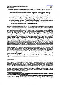
extent the rise in portfolio capital, indicating higher (foreign) investor confidence (lower underlying uncertainty), boosts the relative attraction of the country for direct investment. UNCTAD (1999) moreover suggests that FDI is positively correlated with portfolio investment. One may argue that lagged FDI is also a significant factor of FDI in a dynamic context, since it reflects MNEs’ confidence in economic fundamentals and political environment is an important attractor for FDI, as documented in Busse and Hefeker (2005). In our study, portfolio investment however represents a measure of foreign investor confidence. In addition, using dynamic panel data model, the number of individuals for which data is available (N) is assumed to be large whilst the number of time periods for which data is available (T) is assumed to be small, and asymptotic properties are considered as N becomes large with T fixed (Bond (2002); Baum (2006)); in our sample, N (16) is low relative to T (13) (typically, for GMM, N > 40 and T ≤ 5). In our estimation, we expect positive coefficients on the exchange rate level, manufacturing/GDP ratio, GDP growth, the number of telephone mainlines, share of portfolio investment and exports in GDP. Other coefficients are expected to be negative. We collect annual aggregate data representing those variables for the estimation. In the selection and transformation of most of our data, we follow established practice in the field of research. The data covering 1990-2002 for 16 emerging market countries are selected from International Monetary Fund (2003) on basis of data availability. The countries consist of 8 Latin American countries (Bolivia, Chile, Colombia, Costa Rica, Dominican Republic, Paraguay, Uruguay, and Venezuela), 5 countries from Asia (China, Malaysia, Pakistan, the Philippines, and Thailand), and 3 African countries (Morocco, South Africa, and Tunisia). Net US FDI (constant 2000, Billions of US dollar) to the countries is available from Bureau of Economic Analysis at the US Department of Commerce, and treated as the dependent variable. We use balance of payments data to construct the dependent variable but are aware that the data represent financial flows generated by MNEs, and do not totally represent MNEs’ real activity (Lipsey (2001)). Due to data limitation in developing countries, most of the empirical studies (see, for example, Lucas (1993); Goldberg and Klein (1998); Tuman and Emmert (1999); Wezel (2003)) construct the dependent variable based on the balance of payment data. One may ask a question relating to the dependent variable. It is because the FDI data is in US dollar. If a currency depreciates, then an investment of a given investment size (in local currency) now requires fewer US dollar. This would mean that local currency devaluation would be negatively associated with FDI by definition. The negative relationship, on one hand, may exist in an exceptional case – FDI in an economy giving very limited investment opportunity to investors. Under this circumstance, inflows of FDI would not rise. On the other hand, we concentrate on US FDI in emerging markets, which provide many chances for FDI (Wells and Wint
9
(2000)). The devaluation advantage (the wealth effect as presented in Froot and Stein (1991)) would stimulate new FDI projects by US investors or make US MNEs change their investment plans to undertake FDI in the emerging market countries. Figure 1 presents US FDI trends in the countries. In the 1990s, US FDI to the countries fell rapidly owing largely to falling investments in Latin America. To some extent, the decline was attributed to cyclical movements reflecting, among other things, growth trends in the world economy and fallout from the bursting of technology and telecommunications bubble. At the same time, regional and domestic growth prospects affected FDI. On the other hand, following the 1997 Asian economic crisis, the acquisitions of distressed banking and corporate assets surged in several Asian countries. Driven by market seeking and efficiency seeking FDI, direct investment in Asia increased in the late 1990s (IMF (2003)).
Net FDI Flows from the United States to the Emerging Market Countries (constant 2000, Millions of US dollars) 20, 000
15, 000
10, 000
5, 000
0 20
20
20
19
19
19
19
19
19
19
19
19
19
02
01
00
99
98
97
96
95
94
93
92
91
90
-5, 000 The Emerg ing Market Countries
The Latin Ame rica Countries
Th e Asian Countries
The African Countries
Source: Bureau of Economi c Analysis, US Department of Commerce and Author’s Computation
Figure 1
10
The independent variables are measured as: 1.
Real effective exchange rate indices (REER, 2000=100) are from International Financial Statistics, International Monetary Fund (IMF) through World Development Indicators (WDI) 2004. The IMF defines REER as nominal effective exchange rate4 (NEER) adjusted for relative movements in national price indicators (CPI) of a home country and selected countries.
2.
Average official bilateral exchange rates (local currency unit against US dollar) are from WDI 2004. They are adjusted by CPI (2000=100) of host countries to acquire real exchange rates (see Cushman (1985,1988); Froot and Stein (1991); Klein and Rosengren (1994)).
3.
Manufacturing (MNU) as a share of GDP (constant 2000, US dollar) is from WDI 2004 as a proxy of industrialisation (see Wheeler and Mody (1992)).
4.
Inflation (INF), measured as percentage annual growth of GDP deflator, is from WDI 2004 as a proxy of macroeconomic conditions (see Schneider and Frey (1985); Tuman and Emmert (1999)).
5.
Exports of goods and services (EXP) as a ratio of GDP (constant 2000, US dollar) are from WDI 2004 as a proxy of export potential (see, for example, Singh and Jun (1995); Aseidu (2002)).
6.
GDP per capita (PGDP; constant 2000, US dollar) is from WDI 2004 as a proxy of labour costs (see Cohen (1991)). While this is admittedly a rough proxy it may not be too problematic in our cross-country context, where differences in labour costs across country can be expected to be highly correlated with differences in GDP per capita.
7.
Portfolio investment (current, US dollar) is from WDI 2004. It is adjusted by GDP (current, US dollar) to obtain portfolio investment (PORT)/GDP ratio as a proxy of foreign investors’ confidence.
8.
Data on number of telephone mainlines (TEL) extracted from WDI 2004, utilised as a proxy of infrastructure (see Aseidu (2002)).
9.
GDP growth (GGDP; constant 2000, US dollar) is from WDI 2004, used as a proxy of market potential (see, for example, Gastanaga et al. (1998); Neumayer and Spess (2005)).
Tables 1 and 2 provide descriptive statistics and the correlation of those variables. 4
The IMF defines NEER as a ratio of period average exchange rates currency in question (index) to a trade weighted geometric average of exchange rates for selected country currencies.
11
Table 1: Descriptive statistics Sample: 16 countries and 1990-2002 Variable
Mean
Max
Min
S.D.
FDI (Millions of US dollars)
522.65
11320.03
-1586.85
1406.56
FXD
500.48
4,822.20
1.10
999.63
REER
95.96
133.83
43.87
14.87
GGDP
3.95
14.20
-11.03
4.12
PGDP
2408.76
6377.73
363.58
1596.68
MNU/GDP
20.57
35.39
8.93
5.97
INF
12.95
115.52
-4.04
16.71
TEL
91.97
282.91
5.93
65.20
0.47
32.88
-7.27
2.75
34.07
124.41
14.53
20.10
PORT/GDP EXP/GDP
Source: the US Department of Commerce, WDI 2004 and the author’s computation
Table 2: Correlation matrix Sample: 16 countries and 1990-2002 FDI FDI
∆REER
FXD
TFXD
GGDP
PGDP
MNU/GDP
INF
TEL
PORT/GDP
∆REER
0.19
1
FXD
0.25
0.07
1
TFXD
-0.02
-0.19
0.04
GGDP
0.12
0.31
-0.18
-0.25
1
PGDP
0.25
0.12
0.21
-0.04
-0.15
1
-0.02
-0.02
-0.37
0.05
0.38
-0.15
1
INF
0.30
0.13
0.33
0.16
-0.15
0.33
-0.18
1
TEL
0.08
0.03
0.08
-0.01
-0.13
0.86
-0.01
0.13
1
0.03
0.12
0.01
-0.21
-0.03
-0.02
-0.03
0.04
-0.08
1
-0.01
0.11
0.28
0.08
0.12
0.26
0.45
-0.21
0.21
-0.18
MNU/GDP
PORT/GDP EXP/GDP
EXP/GDP
1
1
1
Source: the US Department of Commerce, WDI 2004 and the author’s computation
12
4.
Econometric Analysis and Results
We firstly estimate equation (5) by employing (within-groups) fixed and random effects (or pooled OLS estimation if summation of estimates of unobserved effect equals zero) to allow for country specific time invariant effects. Fixed effects model is built on an assumption that there is correlation between country specific factors (unobserved specific effects) and independent variable(s). In presence of such correlation, fixed-effects model generates consistent estimators while random effects estimation provides inconsistent coefficients of regressors. If the correlation is zero, random effects estimation then generates consistent and efficient estimators whilst estimators given by fixed effects model are still consistent but inefficient (Wooldridge (2002)). The Hausman test (Baltagi (2001)) is used to justify which technique is more appropriate and, in our case, the test shows a preference for the fixed effects technique. We also check for first-order autocorrelation of the residuals by the LM test. If the errors are not independent and identically distributed (iid) (generating inefficient estimators (Beck and Katz (1995)), fixed-effects with firstorder autocorrelation disturbances estimation5 (Baltagi and Li (1991)) is employed (to remedy the problem). We finally perform a robustness check of regional effects on FDI determination by dividing the countries into two regions: Latin America and Asia. Tables 3 and 4 report estimated coefficients of the independent variables on the (net) US inward FDI to the emerging market countries and the Latin American and Asian countries for the 1990-2002 period. In the final column in Table 3, based on random effects estimation, the results reveal a positive association between FDI inflows and local currency depreciation. Industrialisation degree (MNU/GDP ratio) and market potential (real GDP growth) of host country are positively correlated with inflows of FDI. The estimated coefficients are statistically significant at 5 percent level. The other independent variables are not statistically significant. The Hausman test is undertaken to check presence of correlation between country specific factors and the independent variables. Its statistic of 85.48 is greater than the 5% critical value of the chi-squared distribution with 10 degrees of freedom, showing for the data fixed-effects estimation is more appropriate than random effects estimation (since the correlation is not equal to zero). This allows us to perform estimation again with fixed-effects. Fixed effects estimation results (192 observations) are presented in Table 3. The estimates reveal negative responses of the FDI inflows to expectations of local currency devaluation and local currency volatility. The expected positive response of FDI inflows to depreciation of local currency is also shown. The estimated coefficients of these variables are statistically significant at 5 percent level. In addition, the results provide evidence that high inflation discourages FDI inflows. An increase in foreign investors’ confidence encourages inward FDI. The estimated 5
It is implemented using STATA.
13
coefficients are statistically significant at 10 percent level. The other coefficients are statistically insignificant.
Table 3: Basic estimation results, 1990-2002 Dependent variable: FDI
VARIABLES
FIXED EFFECTS WITH
FIXED
RANDOM
AR(1) DISTURBANCES
EFFECTS
EFFECTS
∆ log of REER
-0.83(0.08)
-0.74(0.13)
-0.54(0.07)
-1.92(0.01)
-0.61(0.68)
FXD (logged)
5.76(0.00)
6.02(0.00)
5.83(0.00)
6.61(0.00)
0.26(0.03)
TFXD (logged)
-6.28(0.01)
-6.64(0.04)
-6.49(0.01)
-7.95(0.00)
-0.14(0.91)
MNU/GDP
-0.04(0.58)
-0.06(0.43)
-0.04(0.61)
0.03(0.66)
0.10(0.01)
INF
-0.01(0.07)
-0.01(0.87)
-0.02(0.08)
-0.01(0.09)
-0.01(0.91)
EXP/GDP
-0.01(0.91)
-0.01(0.91)
-0.01(0.54)
-0.01(0.16)
-0.01(0.49)
PGDP (logged)
2.99(0.18)
3.32(0.14)
3.11(0.17)
3.69(0.11)
1.17(0.12)
PORT/GDP
0.03(0.08)
0.03(0.10)
0.02(0.06)
0.08(0.09)
0.04(0.38)
-0.65(0.21)
-0.41(0.44)
-0.67(0.19)
-0.47(0.17)
-0.39(0.17)
0.01(0.83)
0.01(0.95)
0.01(0.89)
0.02(0.26)
0.06(0.02)
-40.33(0.00)
-41.51(0.00)
-41.43(0.00)
-
-9.53(0.01)
0.41
0.14
TEL (logged) GGDP Constant TIME ∆REER*TFXD (logged) Coefficient of determination
-0.47(0.16) -0.25(0.04)
0.34
0.30
0.21
Hausman test statistic
85.48(0.00)
LM test statistic
179.65
Koenker-Bassett test statistic Number of observations
0.89(0.55)
176
176
176
192
192
Notes: The figures in parentheses are P-values (significant coefficients in bold); the 5% critical value of Chi-squared distribution with 1 degree of freedom is 3.84.
14
We undertake the LM test for the fixed-effects model to check for first-order autocorrelation.6 The calculated test statistic is greater than the 5% critical value of the chi-squared distribution with 1 degree of freedom. As a result, we reject the null hypothesis of no first-order autocorrelation. To remedy the problem, the fixed effects estimation allowing for first-order autocorrelation is used (176 observations). In line with the hypotheses, findings (as presented in Table 3) indicate that an expected devaluation of local currency lowers current inward FDI; FDI rises when devaluation occurs; volatile exchange rate discourages FDI. The estimated coefficients are statistically significant at 10 percent level. The coefficients on inflation and portfolio investment also turn out to have the expected signs (statistically significant) in this regression. These suggest that a rise in foreign investor’s confidence and lower inflation in a host country stimulate inflows of FDI. The results are broadly consistent with prior expectations and with the evidence found in previous studies of FDI determination such as Schneider and Frey (1985) and Tuman and Emmert (1999). From the regression, however, there is no evidence that other independent variables have any impacts on US FDI inflows. To test the hypothesis that the 1997 economic crisis may decrease inflows of FDI to the emerging markets as found in Siamwalla (2004), in equation 5 we include a time dummy variable (TIME), which equals to 1 if the period is 1997-2002 and 0 otherwise (see second column in Table 3). There is no evidence that the economic crisis has any impact on US MNEs decision to undertake FDI in the emerging markets. In this regression, the estimated coefficient of exchange rate expectation is not statistically significant whilst the impacts of foreign currency devaluation and volatility of the exchange rate on the inward FDI are comparable to those obtained before: local currency depreciation stimulates FDI and volatile exchange rate discourages FDI, as Froot and Stein (1991), Chakrabarti and Scholnick (2000) and Campa (1993) argue. It turns out that inflation has no explanatory power on US MNEs decision but foreign investor’s confidence, measured by portfolio capital/GDP ratio, has a positive impact on the inward FDI. The other independent variables are statistically insignificant. Finally, we examine whether exchange rate expectations interact with exchange rate volatility to affect the FDI inflows. Carlson and Osler (2000), who develop a theoretical model highlighting a positive connection between rational expectations and exchange rate volatility, argue that speculative activities in an economy in which all agents are rational, have identical priors and have access to identical information can increase exchange rate variation. On the other hand, Honohan (1985) documents that in a rumor-prone foreign exchange market volatile exchange rate generates large forecasting errors since professionals abandon their view and concentrate instead on guessing what the amateurs are going to do. With the importance of the expectations and volatility interaction, we thus include the interaction variable (∆REER*TFXD) in equation 5 (see first column in Table 3). Including the interaction term improves the overall performance of the regression (R2 = 0.34). Results show that the estimated coefficient of the interaction variable 6
We perform the Koenker-Bassett test to check for the heteroscedasticity problem; however, the calculated test statistic suggests homoscedastic errors.
15
(-0.25) is negative and statistically significant. This implies that given change in REER, the greater is volatility the greater the extent to which FDI is discouraged. In addition, exchange rate expectations give weight on exchange rate variation. If devaluation is expected (∆REER > 0), volatility of exchange rate lowers FDI, as found in Campa (1993). In case of expected appreciation (∆REER < 0), the variation discourages FDI if change in REER is between 0 and -3.32 otherwise the volatility stimulates FDI7, as Cushman (1985, 1988) and Goldberg and Kolstad (1995) argue. Previous results are largely confirmed in this regression. The estimated coefficients on change in REER and transitory component of exchange rate are negative and statistically significant whilst the level of exchange rate has positive and statistically significant coefficient. In line with our hypotheses, an expected devaluation of foreign currency lowers current inward FDI; FDI increases when depreciation occurs; volatility of exchange rate discourages direct investment in general. Higher inflation decreases the FDI inflows, as found in the previous literature. The coefficient on portfolio capital/GDP ratio is positive and statistically significant. This confirms that foreign investor’s confidence stimulates FDI to emerging markets, as discovered in previous regression. Regional Effects on FDI Inflows The three separate exchange rate effects on FDI may quantitatively differ across regions. The 1997 economic crisis has a significant and direct impact on level of exchange rates in Asian countries (Siamwalla (2004)). In addition, after the crisis some of the countries adopted floating exchange rate regime (Waiquamdee et al. (2005)). Therefore, it is important to test the regional effects on US FDI inflows. We estimate a version of equation (5) which includes a dummy variable for Asian countries interacted with the core explanatory variables. FDIi,t = β0 + β 1 ∆ REERi,t + β 2 FXDi,t + β 3 TFXDi,t+ β 4 Xi,t+ β5ASIA + β6 ASIA* ∆ REERi,t + β7 ASIA*FXDi,t + β8 ASIA*TFXDi,t+ µ i + ε i,t (6)
where ASIA is a dummy variable that is 1 for Asian countries and 0 otherwise. To have a sensible comparison group we include Latin American countries in this sample (i.e. omit the African countries). Using fixed effects estimation, the previous results are largely confirmed but Asia exhibits some differences compared to Latin America (the samples are too small to reliably estimate each region separately). The LM test however suggests misspecification due to first-order autocorrelation.8 The calculated test statistic is
7
∂ FDI/ ∂ TFXD = -0.83 - 0.25*∆REER. In case of expected appreciation, the exchange rate variation effect on FDI is negative if ∆REER is between 0 and -3.32.
8
The Koenker-Bassett test statistic shows that the errors are homoscedastic.
16
greater than the 5% critical value of the chi-squared distribution with 1 degree of freedom so we can reject the null hypothesis of no first-order autocorrelation9; and, we re-estimate by fixed-effects with AR(1) disturbances. The findings for fixed effects allowing for first-order autocorrelation show that the results on inflation and market potential variables are broadly consistent with prior expectations and with the evidence found in other studies of FDI determination, such as Schneider and Frey (1985), Gastanaga et al. 1998, Tuman and Emmert (1999) and Wezel (2003). Inflation discourages whereas market potential encourages inflows of FDI. In line with the hypotheses, exchange rate volatility, local currency appreciation and expectations of local currency depreciation all discourage FDI flows into both Latin America and Asia. The other independent variables are statistically insignificant. An estimate of the extent of extra FDI to Asia compared to Latin America is 2.93.10 In Latin America, the expectation in local currency devaluation (increasing REER) coefficient is –4.0, but for Asian countries it is –9.95 (i.e., β1 + β12 = -4+-5.95). Thus, the impact of expected local currency devaluation is considerably greater for Asian countries. In contrast, the impacts of volatile exchange rates and local currency appreciation effects are slightly weaker for Asian countries. As a result, for both Latin American and Asian countries, the impacts of exchange rate devaluation, volatility of exchange rate and the expectations on US FDI inflows to emerging markets are consistent with those reported in Table 3, albeit with some regional variations.
9
Using pooled OLS estimation, the estimates show positive responses of the FDI inflows to GDP growth in all of the countries. However, in the Latin American countries, local currency devaluation increases FDI inflows. The remaining variables are not statistically significant. The F-test statistic of 18.76 is greater than the 5% critical value of the F-distribution with 12 and 130 degrees of freedom, indicates that fixed effects estimation is more appropriate than pooled OLS estimation for the data. 10
∂ FDI / ∂ ASIA = β11 + β12 ∆ REER + β13FXD + β14TFXD, evaluated at mean values of variables.
17
Table 4: Regression results: is Asia different? Dependent variable: FDI
VARIABLES
∆ log of REER (β1)
FIXED EFFECTS WITH AR(1) DISTURBANCES
OLS
FIXED EFFECTS
-4.00(0.01)
-3.36(0.02)
1.37(0.49)
9.38(0.00)
9.58(0.00)
0.14(0.03)
TFXD (logged, β3)
-9.05(0.00)
-10.87(0.00)
1.74(0.38)
MNU/GDP (β4)
-0.07(0.27)
-0.11(0.88)
-0.03(0.37)
INF (β5)
-0.02(0.01)
-0.01(0.01)
0.01(0.16)
EXP/GDP (β6)
0.01(0.89)
0.01(0.68)
-0.02(0.03)
PGDP (logged, β7)
5.24(0.20)
4.69(0.17)
1.42(0.39)
PORT/GDP (β8)
0.06(0.23)
-0.02(0.74)
-0.03(0.73)
TEL (logged, β9)
-0.99(0.11)
-0.87(0.12)
-0.64(0.14)
GGDP (β10)
0.04(0.09)
0.05(0.05)
0.07(0.05)
ASIA (β11)
6.44(0.01)
-
2.76(0.01)
ASIA*∆ log of REER (β12)
-5.95(0.04)
6.38(0.01)
4.22(0.28)
ASIA*FXD (logged) (β13)
-0.79(0.08)
-7.29(0.01)
-0.47(0.07)
0.37(0.00)
1.93(0.06)
-3.67(0.41)
-67.76(0.00)
-
-7.81(0.00)
0.48
0.55
0.26
FXD (logged, β2)
ASIA*TFXD (logged) (β14) Constant Coefficient of determination F-test: H0: β1+ β12 = 0
10.56(0.01)
F-test: H0: β2+ β13 = 0
3.19(0.07)
F-test: H0: β3+ β14 = 0
24.29(0.00)
F-test statistic
18.76(0.00)
LM test (Chi-squared) statistic
143.43
Koenker-Bassett test statistic Number of observations
0.55 (0.17) 143
156
156
Notes: The figures in parentheses are P-values (significant coefficients in bold); the 5% critical value of Chi-squared distribution with 1 degree of freedom is 3.84.
18
5.
Concluding Remarks
This paper investigates the effects of exchange rates, exchange rate expectations, and exchange rate volatility on (net) US FDI to 16 emerging market countries. Our empirical estimation starts from, and extends, a model by Chakrabarti and Scholnick (2002). We employ annual aggregate data over the period of 1990-2002. Our hypotheses based on the model are that expectations of local currency appreciation and local currency depreciation may stimulate inward FDI. In addition, we expect that exchange rate volatility has probably a significant role on FDI inflows. Our results can be summarised as: 1.
There is robust evidence of the positive (negative) relationship of local currency devaluation (appreciation) and FDI inflows.
2.
There is evidence of the negative (positive) relationship of expectations of local currency depreciation (appreciation) and FDI inflows. The result implies that FDI in the countries is increasingly being undertaken to service domestic demand for finance, telecommunications, wholesaling, and retailing rather than to tap cheap labour. This supports an argument by IMF (2003).
3.
There is evidence of the negative relationship of volatile exchange rates and FDI inflows.
4.
The interaction variable (∆REER*TFXD) is significant. Given change in REER, the greater is volatility the greater the extent to which FDI is discouraged. In addition, exchange rate expectations give weight on exchange rate variation. If devaluation is expected, a volatile exchange rate discourages FDI. In case of expected appreciation, the variation decreases FDI when change in REER is between 0 and -3.32 otherwise the variability encourages FDI.
5.
We find that economic conditions and foreign investors’ confidence in host countries are significant.
6.
The 1997 economic crisis has no impact on US FDI in emerging markets possibly because the impact is on exchange rates, especially in Asia, which then affect FDI.
Foreign investors in emerging markets do respond to the exchange rate: devaluation attracts FDI (as it reduces the price of assets abroad), although an expected devaluation postpones FDI. US investors are discouraged by volatile exchange rates, perhaps because this is correlated with economic and political uncertainty, which also appears to discourage FDI.
19
Our analysis contributes to the discussion of the impacts of exchange rates on FDI. However, a limitation is the sample used here. The period of study starts from 1990 and the sample is restricted to relatively few countries since REER data are not available for earlier years and for many emerging market countries. The utilisation of longer and/or broader data series would extend and test the results. Another improvement of this paper would be to utilise data from future exchange rate markets and the standard deviation of high frequency (monthly or daily) exchange rate data to re-analyze the effects of exchange rate expectations and volatility on FDI inflows. The country-level analysis moreover has some limitations, particularly when MNEs have different FDI objectives. Suppose two types of MNEs with two different FDI objectives exist in a host country. One is interested in low cost production (export-oriented FDI). The other is interested in domestic sales (marketseeking FDI). Under such circumstances, the country-level analysis cannot clearly clarify the FDI types (in the country) by capturing the exchange rate expectation impact on inward FDI. As a consequence, this investigation indicates the need to undertake the firm-level analysis, which requires detailed information on firm activities.
20
APPENDIX A summary of Hodrick-Prescott filter approach According to Hodrick and Prescott (1997), this technique widely used among economists is a smoothing method to receive a smooth estimate of the long-term trend component of a series. Technically, they consider a given time series yt, which is seasonally adjusted, is the sum of a growth component gt, which varies ‘smoothly’ over time, and a cyclical component ct: yt = gt + ct for t = 1, 2, …, T.
Their measure of the smoothness of the {gt} path is the sum of the squares of its second difference. The ct are deviations from gt but their average is near zero over long time periods. These considerations lead to the following programming problem for determining the growth components:
Min gt
T −1 T 2 c + λ ((g t +1 − g t ) − (g t − g t −1 ))2 ∑ ∑ t t =1 t =1 t =2
T
where ct = yt – gt. The parameter λ is a positive number, which penalises variability in the growth component series. The larger the value of λ , the smoother is the solution series. For a sufficiently large λ , at the optimum all the gt+1 - gt must be arbitrarily near some constant β and therefore the gt arbitrarily near g0 + β t. This implies that the limit of solutions to program the function as λ approaches infinity is the least squares fit of a linear time trend model.
21
REFERENCES Asiedu, E. (2002). ‘On the Determinants of Foreign Direct Investment to Developing Countries: Is Africa Different?’, World Development, Vol. 30(1), pp. 107-119. Baltagi, B.H. and Li, Q. (1991). ‘A Transformation that will circumvent the problem of autocorrelation in an error-component model’, Journal of Econometrics, Vol. 48, pp. 385-393. Baltagi, B.H. (2001). Econometric Analysis of Panel Data, 2nd ed. Chichester: John Wiley. Baum, C.F. (2006). An Introduction to Modern Econometrics Using STATA, Texas: A STATA Press Publication. Beck, N. and Katz, J.N. (1995). ‘What to do (and not to do) with time-series crosssection data’, American Political Science Review, Vol. 89, pp. 634-637. Blonigen, B.A. (1997). ‘Firm – specific Assets and the Link between Exchange Rates and Foreign Direct Investment’, American Economic Review, Vol. 87, pp. 447-465. Blonigen, B.A. (2005). ‘A Review of the Empirical Literature on FDI Determinants’, NBER Working Paper No. 11299, National Bureau of Economic Research, April 2005. Bond, S. (2002). ‘Dynamic Panel Data Models: A Guide to Micro Data Methods and Practice,’ Cemmap Working Paper CWP09/02, The Institute for Fiscal Studies, April 2002. Bureau of Economic Analysis (2004). US-International Transactions Account Data, available from http://www.bea.gov/bea/di1.htm/. Busse, M. and Heferker, C. (2005). ‘Political Risk, Institutions and Foreign Direct Investment,’ HWWA (Institute of International Economics) Discussion Paper No. 315, (HWWA) Institute of International Economics, April 2005. Campa, J.M. (1993). ‘Entry by Foreign Firms in the United States under Exchange Rate Uncertainty’, Review of Economics and Statistics, Vol. 75, pp. 614-622. Carlson, J.A. and Osler, C.L. (2000). ‘Rational speculators and exchange rate volatility’, European Economic Review, Vol. 44, pp. 231-53. Chakrabarti, R. and Scholnick, B. (2002). ‘Exchange Rate Expectations and Foreign Direct Investment Flows’, Weltwirtschaftliches Archiv, Vol. 138(1), pp. 1-21. Chinn, M.D. (2000). ‘Before the Fall: Were East Asian Currencies Overvalued?, Emerging Markets Review, Vol. 1(2), pp. 101-26. Chinn, M.D. (2005). ‘A Primer on Real Effective Exchange Rates: Determinants, Overvaluation, Trade Flows and Competitive Devaluation’, NBER Working Paper No. 11521, National Bureau of Economic Research, July 2005.
22
Cohen, D. (1991). ‘Slow Growth and Large LDC Debt in the Eighties: An Empirical Analysis,’ CEPR Discussion Paper No. 461, The Center for Economic Policy Research, January 1991. Cushman, D.O. (1985). ‘Real Exchange Rate Risk, Expectations, and the Level of Direct Investment’, Review of Economics and Statistics, Vol. 67, pp. 297-308. Cushman, D.O. (1988). ‘Exchange – rate Uncertainty and Foreign Direct Investment in the United States’, Weltwirtschafiliches Archiv, Vol. 67, pp. 297-308. Frankel, J. and Froot, K. (1987). ‘Using survey data to test standard propositions regarding exchange rate expectations’, American Economic Review, Vol. 77(1), pp. 133-153. Froot, K. and Stein, J. (1991). ‘Exchange Rates and Foreign Direct Investment: an Imperfect Capital Markets Approach’, Quarterly Journal of Economics, Vol. 196, pp.1191-1218. Gastanaga, V.M., Nugent, J.B. and Pashamova, B. (1998). ‘Host Country Reforms and FDI Inflows: How Much Difference do they Make?’, World Development, Vol. 26(7), pp. 1299-1314. Goldberg, L.S. and Kolstad, C.D. (1995). ‘Foreign Direct Investment, Exchange Rate Variability and Demand Uncertainty’, International Economic Review, Vol. 36, pp. 855-873. Goldberg, L.S. and Klein, M. (1998). ‘Foreign Direct Investment, Trade and Real Exchange Rate Linkages in Developing Countries’, in Glick, R., eds., Managing Capital Flows and Exchange Rates: Perspectives from the Pacific Basin, pp. 73-100. Cambridge: Cambridge University Press. Goldfajn, I. and Valdes, R.O. (1999). ‘The Aftermath of Appreciations’, The Quarterly Journal of Economics, Vol. 114(1), pp. 229-62. Hodrick, R. and Prescott, E. (1997). ‘Post-war US Business Cycles: An Empirical Investigation’, Journal of Money Credit and Banking, Vol. 29, pp. 1-16. Honohan, P. (1984). ‘Expectation Errors and Exchange-Rate Volatility’, Journal of Macroeconomics, Vol. 6(3), pp. 323-34. International Monetary Fund. (2003). ‘Foreign Direct Investment in Emerging Market Countries’, Report of the Working Group of the Capital Markets Consultative Group, International Monetary Fund, September 2002. Klein, M.W. and Rosengren, E.S. (1994). ‘The Real Exchange Rate and Foreign Direct Investment in the United States: Relative Wealth vs. Relative Wage Effects’, Journal of International Economics, Vol. 36, pp. 373-389. Lipsey, R.E. (2001). ‘Foreign Direct Investors and the Operations of Multinational Firms: Concepts, History and Data’, NBER Working Paper No. 8665, National Bureau of Economic Research, December 2001. Lucas, R.B. (1993). ‘On the Determinants of Direct Foreign Investment: Evidence from East and Southeast Asia’, World Development, Vol. 21(3), pp. 391-406.
23
Neumayer, E. and Spess, L. (2005). ‘Do bilateral investment treaties increase foreign direct investment to developing countries?’, World Development, Vol. 33(10), pp. 1567-1585. Newbold, P. (1995). Statistics for Business and Economics, 4nd ed. New Jersey: Prentice-Hall, Inc. Noorbakhsh, F., Paloni, A. and Youssef, A. (2001). ‘Human Capital and FDI Inflows to Developing Countries: New Empirical Evidence’, World Development, Vol. 29(9), pp. 1593-1610. Schneider, F. and Frey, B.S. (1985). ‘Economic and Political Determinants of Foreign Direct Investment’, World Development, Vol. 13(2), pp. 161-175. Siamwalla, A. (2004). ‘Anatomy of the Crisis’, in Warr, P.G., ed., Thailand Beyond the Crisis (Rethinking South East Asia). Routledge: London. Singh, H. and Jun, K.W. (1995). ‘Some New Evidence on Determinants of Foreign Direct Investment in Developing Countries’, Policy Research Working Paper No. 1531, The World Bank, November 1995. Tuman, J.P. and Emmert, C.F. (1999). ‘Explaining Japanese Foreign Direct Investment in Latin America, 1979-1992’, Social Science Quarterly, Vol. 80(3), pp. 539-555. United Nations Conference on Trade and Development (1999). ‘Foreign Portfolio Investment (FPI) and Foreign Direct Investment (FDI): Characteristics, similarities and differences, policy implications and development impact’, Report of the Expert Meeting on Portfolio Investment Flows and Foreign Direct Investment, United Nations Conference on Trade and Development, June 1999. Waiquamdee, A., Disyatat, P. and Pongsaparn, R. (2005). ‘Effective Exchange Rates and Monetary Policy: The Thai Experience’, Discussion Paper No. 04/2005, the Bank of Thailand, May 2005. Wells, L.T. and Wint, A.G. (2000). ‘Marketing a Country: Promotion as a Tool for Attracting Foreign Investment’, Foreign Investment Advisory Service (FIAS) Occasional Paper 13, International Finance Corporation, April 2000. Wezel, T. (2003). ‘Determinants of German Foreign Direct Investment in Latin American and Asian Emerging Markets in the 1990s’, The Deutsche Bundesbank Discussion Paper (11/03), The Deutsche Bundesbank, April 2003. Wheeler, D. and Mody, A. (1992). ‘International Investment Location Decisions’, Journal of International Economics, Vol. 33, pp. 57-56. Wooldridge, J. M. (2002). Econometric Analysis of Cross Section and Panel Data, London: MIT Press. World Bank (2004). World Development Indicators 2004, available from http://devdata.worldbank.org/dataonline/.
24