Journal of
Economics and Political Economy www.kspjournals.org December 2016
Volume 3
Issue 4
Foreign Direct Investment and Sectoral Performance in Tanzania By Manamba EPAPHRA †aa Abstract. Although it may seem natural to argue that Foreign Direct Investment (FDI) can bridge the investment gap in developing countries’ economy, which in turn foster economic growth, this paper shows that the effects of FDI vary greatly across sectors. In fact, there is a lack of systematic evidence on the actual impact of FDI on the host country. An empirical analysis using time series data spanning from 1970 to 2015 and applying Error Correction Mechanism, suggests that FDI exerts a negative effect on agriculture value added. Unsurprisingly, FDI tends to have a positive effect on manufacturing, construction and transport, storage and communication sectors. Evidence from the mining sector is not clear despite the fact that the sector constitutes a substantial proportion of FDI inflows. The unexpected negative causal relationship between FDI inflows and agricultural sector in Tanzania could be because of the low level of FDI in the sector relative to other sectors. However, it is possible for FDI to be contributing to the GDP through manufacturing, construction and transport, storage and communication sectors and yet not increasing the welfare of the people in the country. Agricultural sector, which constitutes more than 70 percent of the total labour force, contributes, on average, less than 30 percent, in total GDP. Understandably, FDI in the agricultural sector can improve the welfare in the country than FDI in mining and manufacturing sectors. Given the importance of the subject, it is surprising to find that very little effort has been devoted to quantifying the sources of agricultural decline. Keywords. FDI, Sectoral composition, Agricultural sector, Mining sector and Manufacturing sector. JEL. F23, F36, F43
1. Introduction
I
t is widely accepted that FDI has a significant role to play in national development strategies and is viewed as the engine with which to exploit and sustain the competitiveness of resources and capabilities mainly through economic liberalization doctrine. Proponents of FDI argue that FDI plays a significant role in increasing productivity by offsetting the investment and technological gap (Chen & Démurger, 2002; FAO, 2001; and Buckley et al., 2006). It also contributes to improved transfer of technology and skills (Kabelwa, aa
† Department of Accounting and Finance, Institute of Accountancy Arusha, Tanzania. . +255 754399775 .
[email protected]
Journal of Economics and Political Economy 2003, 2004; IMF, 2001) which in turn improve efficiency and economic growth (Blomström & Kokko, 2003). According to IMF (2001), FDI promotes economic growth through raising technological levels, creating new employment opportunities and offering a source of external capital in developing countries. Similarly, Nyankweli (2012) points out that the effect of FDI on the economy includes enhancing the inflow of external resources. In general, FDI has become an important force in both low income and high income economies because of its impact on economic and socio-cultural development as well as livelihoods (Luvanga & Shitundu 2003; UNCTAD 2003, 2004). Likewise, it is shown that FDI works as a means of integrating developing countries into the global market place and increasing the capital available for investment which in turn lead to increased economic growth required for poverty reduction and improvement in living standards (Rutihinda, 2007; Dollar & Kraay, 2002, Dupasquier & Osakwe, 2005). Indeed, policy makers and governments encourage multinational enterprise (MNE) activity as a source of capital and technology and believe that inward FDI flows fill the savings, investment, and production gaps in less developed countries. As a result, FDI is regarded as a means to alleviate resource and skill constraints (Noorbakhsh et al., 2001) through the application of ownership-specific advantages in the form of financial, human resources, technology and knowledge (Dunning, 1993). During the past 20 years there has been a marked increase in both the flow and stock of FDI in the world economy. For example, FDI flows to developing economies increased by 2 per cent to a historically high level in 2014, reaching US$681 billion (UNCTAD, 2015). In Tanzania, with the initiation of economic reforms in 1986, investment interest in the country has grown considerably in all sectors. During the 1995-1998 period, FDI flows were 3.6 times as much as the magnitude registered in the 1970-1994 period. Certainly, the mid 1990s have been characterised by a strong momentum in the economic reform process. FDI net inflows as percent of GDP in the country was, on average, 3 percent of GDP during the 2004-2014 period (Epaphra & Massawe, 2016). Its highest value over the past 20 years was 5.2 in 1999, while its lowest value was 0.2 in 1998. In recent years, the value of FDI inflows increased from US$ 2130.9 million in 2013 to US$ 2141.6 million in 2014. Also, FDI stocks rose to US$ 17013.4 million in 2014 from US$ 14871.8 in 2013, equivalent to an increase of 14.4 percent, despite the fact that the global FDI inflows in 2014 fell by 16 percent, mostly because of the fragility of the global economy, policy uncertainty for investors and elevated geographical risks (UNCTAD, 2015). The current increase in FDI in Tanzania mainly is due to gas discoveries. Meanwhile, during the 2008-2014, South Africa, the United Kingdom and Canada accounted for an average of 70 percent of the total FDI inflows to Tanzania implying that the sources of FDI inflows is inadequately diversified, thus exposing the country to risks emanating from external shocks (Epaphra & Massawe, 2016). Understandably, between 2000 and 20014, Tanzania had one of the strongest growth rates of the non-oil-producing countries in Sub-Saharan Africa. During that period, annual real GDP growth was, on average, 6.6 percent, with 7.2 percent in 2014 (World Bank, 2015). However, per-capita GDP averaging US$ 881.3 over the 2011-2015 period is far from the projected US$ 3,000 by 2025. Indeed, to achieve a status of a middle income country by 2025, Tanzania economy is supposed to grow at about 10 percent per annum. Agriculture, which accounts for JEPE, 3(4), M. Epaphra, p.670-719.
671 671
Journal of Economics and Political Economy the largest share of total labour force records low levels of investment expenditure. For example, the annual FDI inflows to agriculture are lower than that of mining and quarrying and manufacturing which account for 3.4 percent and 8.2 percent share in GDP respectively (Epaphra & Massawe, 2016). As a result, up until 2007, the poverty rate in Tanzania remained stagnant at around 34 percent of the whole population despite a robust growth at an annualized rate of approximately 7 percent. A huge percent of population living below the standard poverty line is that of small scale farmers leaving in rural areas. Thus, growth in agriculture and its productivity are considered essential in achieving sustainable growth and significant reduction in poverty in developing countries. Undoubtedly, limited development and adoption of new production technologies essential for improving productivity by the poor are mostly due to limited income and sources of credit. To this end, FDI is expected to play a significant role in increasing productivity by offsetting the investment and technological gap as it comes with improved technologies. In spite of noticeable impact of FDI on economic growth, however, the FDI flows by activity raise a number of questions at the core of using FDI as a driver of sustainable growth, employment and poverty reduction. During the 1998-2014 period, FDI flows to agriculture, hunting and forestry which employed about 70 per cent of the labour force and contributed 25 percent to GDP was, on average 1.3 percent of total FDI flows while mining sector that employed less than 1 percent of the labour force and contributed 3.4 percent to GDP had 30.5 percent share in total FDI flows during the same period. In fact, the flows of FDI to agriculture sector are less than that of manufacturing and electricity and gas sectors. As a result, Tanzania’s exports tend to shift from traditional commodities such as coffee, cotton, sisal, tea and tobacco towards non-traditional products such as minerals, gold in particular. This means that the use of FDI in attaining sustainable employment, economic growth and poverty reduction would have substantial effect on the performance of the whole economy. This paper therefore examines the impact of FDI on various sectors of the economy such as agriculture, hunting, forestry, fishing (ISIC A-B), mining (ISIC C), manufacturing (ISIC D), construction (ISIC F) and transport, storage & communication (I) in Tanzania. The choice of the sectors mainly was due to their importance in the economy and availability of time series data. This is very significant because previous studies, for example, Alfaro (2003) concludes that the contribution of FDI to growth depends on the sector of the economy where the FDI operates. He claims that FDI inflow to the manufacturing sector has a positive effect on growth whereas FDI inflow to the primary sector tends to have a negative effect on growth while its effect on services sector is not so clear. The paper uses time series data spanning from 1970 to 2015. The justification of this paper is based on the assumption that good performance of FDI is reflected in growth of the host country and improvement in the living standards of its people. This is largely contributed to improvement in sectoral performance and one of them being agriculture which employs more than half of the total working class and its contribution in GDP is substantial.
JEPE, 3(4), M. Epaphra, p.670-719.
672 672
Journal of Economics and Political Economy 2. Nature of the Economy and Sectoral Distribution of Foreign Direct Investment 2.1. Macroeconomic Performance During the 1970-2015 period, the Tanzanian economy experienced mixed performance. Real GDP growth, inflation, real exchange rate and FDI have been characterized by fluctuations, partly a result of economic policies pursued by Tanzania under a public sector-led economy embedded in the 1967 Arusha Declaration, and partly a result of exogenous factors, including deterioration in the terms of trade in the late 1970s and early 1980s, the collapse of the East African Community in 1977, and the war with Uganda’s Iddi Amin during 1978-1979. The fall in the prices of exports such as sisal, tea and cotton and the rise in price of imports such as oil crisis of 1973-1974 and oscillating currency exchange rates also contributed to these fluctuations. However, during the last decade, economic performance has remained stable and strong. For example, the annual mean of real GDP growth increased from 6.1 percent during the 2006-2010 period to 6.9 percent during the 2011-2015 period despite the fact that inflation rose from annual mean of 8.6 percent during 2006-2010 period to 9.7 percent during the 2011-2015 period (Table 1). Nonetheless, over the past few years, inflation has stabilized at single digits, declining from an annual rate of 34 percent in 1994 to 5.6 percent in 2015 mainly due to prudent fiscal and monetary policy measures. Overall performance of macroeconomic variables including trade, gross fixed capital formation, FDI and tax revenue during the 2011-2015 period was stable. Indeed, annual mean of tax revenue-to-GDP ratio rose from 9.1 percent during the 2001-2005 period to an annual mean of 11.8 percent over the 2011-2015 period. Table 1. Selected Economic Indicators, 1970-2015 pGDP, US$ Growth GFCF RER TL
Population FDI Tax Revenue Expenditure
19701975 231.0 4.7 41.7 723.5 46.9 12.0 3.2 0.1 18.2 24.65
19761980 413.7 2.9 40.6 579.5 37.1 13.6 3.1 0.1 17.9 26.8
19811985 545.0 1.1 21.0 409.9 21.2 30.2 3.1 0.1 16.4 26.1
19861990 292.7 3.9 20.4 1235.7 28.8 31.1 3.1 0.0 10.2 12.0
19911995 256.8 4.0 27.7 1624.6 42.2 27.5 3.2 0.6 10.0 13.6
19962000 366.7 4.2 20.9 1164.4 24.2 12.7 2.6 2.1 9.4 11.9
20012005 424.5 7.1 24.8 1435.0 27.6 5.1 2.8 3.1 9.1 16.0
20062010 604.7 6.1 37.3 1475.6 44.9 8.6 3.1 3.8 9.8 17.2
20112015 881.3 6.9 42.6 1299.4 51.8 9.7 3.2 4.3 11.8 18.5
Notes: pGDP: real per capita GDP; Growth: real GDP annual growth rate; GFCF: gross fixed capital formation, percent of GDP; RER: real exchange rate; TL: exports plus imports, percent of GDP; : Inflation; POP: population growth rate; FDI: foreign direct investment; Tax revenue-to-GDP ratio; Government expenditure-to-GDP ratio. Source: computed using data from World Bank and Bank of Tanzania (Various issues)
The strong economic performance in recent years was driven mainly by construction, information and communication and wholesale, retail trade, restaurants and hotels sectors (Table 2). The construction activity grew by 14 percent in 2015 (BoT, 2014) and accounted for an annual mean of 10.9 percent of GDP over the 2011-2015 period (Table 2). The improved performance of construction activity was attributed to construction and rehabilitation of bridges, buildings, road network, airport, as well as acquisition of ferries (BoT, 2015). The value added of transport, storage and communication as percent of GDP rose from JEPE, 3(4), M. Epaphra, p.670-719.
673 673
Journal of Economics and Political Economy annual mean of 8.1 percent over the 2006-2010 period to annual mean of 9.4 percent during the 2011-2015 period reflecting increased number of mobile phone subscribers and internet users, as well as investment resulting from technological innovations (BoT, 2014). Cargo handling at Dar es Salaam port also improved owing to measures implemented to reduce time for cargo clearance. This supportive physical infrastructure and a favourable business environment represent important pre-requisites for FDI-led industrialization. Table 2. Value Added, Percent of GDP (2005 Prices), 1970-2015 Sector ISIC A-B ISIC C-E ISIC D ISIC F ISIC G-H ISIC I ISIC J-P TVA
19701975 29.63 12.43 10.37 4.82 13.71 9.07 19.97 100
19761980 27.52 12.15 10.50 3.64 11.93 8.84 25.40 100
19811985 28.62 10.29 8.00 2.85 11.00 7.70 31.54 100
19861990 30.94 8.98 6.85 3.64 11.52 7.06 31.01 100
19911995 33.00 9.19 6.80 6.05 11.09 7.10 26.76 100
19962000 32.59 9.75 6.69 6.39 11.03 7.35 26.20 100
20012005 30.20 11.14 6.96 7.30 11.20 7.45 25.76 100
20062010 26.86 11.49 7.89 9.26 11.67 8.09 24.75 100
20112015 23.89 11.45 8.06 10.91 11.85 9.42 24.42 100
Notes: ISIC A-B: Agriculture, hunting, forestry, fishing; ISIC C-E: Mining, manufacturing, utilities; ISIC D: Manufacturing; ISIC F: Construction; ISIC G-H: Wholesale, retail trade, restaurants and hotels; ISIC I: Transport, storage & communication; ISIC J-P: Other Activities. Source: Computed using data from United Nations Statistics Division (2016)
Along with economic reforms and recovery that started in 1986, priority spending aimed at promoting high economic growth and improving social services was channeled to investment in socio-economic sectors such as infrastructure, agriculture, health and education. As a result reforms were supported by large inflows of foreign aid and technical assistance. In particular, FDI inflows-to-GDP ratio rose from 0.01 percent over the 1986-1990 period to 4.3 percent during the 2011-2015 period. Also, during the same period the degree of openness increased from 28.8 percent to 51.8 percent after several years of fluctuation chiefly due to policy changes (Table 2). During the early period of reforms and recovery macroeconomic stability was not achieved mainly due to the government’s inability to control credit expansion to public enterprises, massive tax exemptions, poor revenue collections, and tax evasion. In the 1980s and early 1990s economic performance was extremely weak, with growth in GDP often less than the growth in population. Similarly, export performance remained strong in the recent years, driven by gold and tourism receipts (BoT, 2015). This also implies that the country does not only attract FDI but also it engages in outward investment in foreign markets. Besides, exportation has a relatively low-risk to enter a foreign market because it does not involve actual presence in the target market (Shenkar, 2007). Nevertheless, exporting does not enable firms to maintain control over foreign production and operations. 2.2. Sectoral Distribution of Foreign Direct Investment The World Investment Report (2015) shows that in 2014, the top five FDI recipients were Mozambique with US$4.9 billion, Zambia with US$2.5 billion, the United Republic of Tanzania with US$2.1 billion, the Democratic Republic of the Congo with $2.1 billion and Equatorial Guinea with $1.9 billion. These five countries accounted for 58 per cent of total FDI inflows to LDCs reinforced by the export specialization of these countries (UNCTAD, 2015). Indeed, FDI inward JEPE, 3(4), M. Epaphra, p.670-719.
674 674
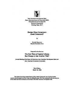
Journal of Economics and Political Economy stock in Tanzania in 2014 was as much as US$ 17 mainly due to gas discoveries and mineral exports. In the same line, improved macroeconomic performance, political stability and market liberalization since the second half of 1990s have led to a surge in investor interest and have encouraged the inflow of foreign capital. During the 1980-2015 period, the FDI inflows and stocks have increased steadily (Figure 1). This FDI performance has followed the developments in the political economy, reflecting the wide spread economic liberalization, Mineral Policy of 1997, enactment of the Mining Act of 1998, the Mining Act of 2010, the Investment Policy and Act of 1997 and other promotional efforts by Government. Indeed, in the second half of the 1990s, FDI grew much faster than the economy. The share of FDI stock as a percent of GDP reflects the importance of FDI activity in the country’s productive process and shows the potential impact of FDI stock (Portelli, 2005).
Figure 1. Real GDP Growth, FDI, Inflows and Stocks Source: Computed using data from UNCTAD, WIR (2015)
Tanzania also compares well to its regional African neighbours in terms of total FDI inflows and stocks1 reflecting investment in tourism infrastructure/hotels and mining exploration (URT, 2014) (Tables 3 and 4). This also highlights the importance of foreign investment in total investment for the Tanzanian economy. According to (UNIDO, 2003), Tanzania is gradually assuming a front-runner position in attracting foreign investment in SSA. Indeed, FDI is now considered as an important input for development of the economy. It brings scarce capital needed in the economy that has large current account deficits. It also brings new technology and managerial knowhow to enhance growth and productivity (Kinoshita, 2011). FDI in the nontradable sectors boost current account deficits without contributing to an expansion of export earning capacity while FDI in the tradable sector is associated with higher exports (Kinoshita, 2011). Understandably, economic growth is an essential condition for poverty reduction in Tanzania.
1
The flow of FDI means the amount of FDI undertaken over a given time period (e.g. a year). The stock of FDI means the total accumulated value of foreign owned assets at a given time (which takes into account possible divestment along the way).
JEPE, 3(4), M. Epaphra, p.670-719.
675 675
Journal of Economics and Political Economy Table 3. FDI, Inward Flows (USD Millions) Economy 1980-85 1986-90 Burundi 3.56 1.18 Kenya 28.24 38.36 Rwanda 15.99 15.88 Uganda 0.34 -0.59 Tanzania 8.07 0.33 Source: UNCTAD, WIR (2015)
1991-95 0.79 12.82 3.58 54.25 46.40
1996-00 2.22 39.94 4.35 143.34 251.42
2001-05 0.13 36.39 8.07 242.71 485.82
2006-10 1.10 233.67 116.88 710.17 1026.73
2011-14 10.68 521.96 224.85 1085.56 1825.36
Table 4. FDI, Inward Stocks (USD Millions) Economy 1980-85 1986-90 1991-95 1996-00 Burundi 18.52 28.08 31.99 37.00 Kenya 426.37 576.90 701.05 819.54 Rwanda 0 6.53 45.55 56.98 Uganda 11.60 9.87 102.27 568.24 Tanzania 369.98 382.87 459.4 1585.22 Source: UNCTAD, World Investment Report (2015)
2001-05 46.93 1030.83 64.42 1425.46 3557.98
2006-10 3.49 1886.52 269.36 4185.19 7066.70
2011-14 20.26 3310.95 788.51 8208.21 13891.86
FDI in Tanzania originates from a wide range of countries. The Tanzania Investment Report (2013) shows that the top six source countries for FDI stock in 2012 were United Kingdom, Canada, Switzerland, USA, South Africa and Kenya. These countries accounted for US$ 786.9 million, US$ 308.8 million, US$ 219.4 million, US$ 198.9 million, US$ 148.3 million, and US$ 108.7 million respectively. In 2012, Inflows from South Africa, United Kingdom, Barbados, Canada and Kenya reached US$ 7,423.5 million, equivalent to 58.2 percent of the total stock of FDI (Tanzania Investment Report, 2013). This also implies that in Tanzania, FDI originates from few source countries. FDI flows to Tanzania are categorized into market-seeking FDI, for example, investment in manufacturing of beer, cement and sugar; export-oriented FDI for example investment in mining and textile and FDI in infrastructure and utilities such as energy, port and telecommunication. Table 5 reports the flows and stocks of FDI by activity over the 2008-2012 period in Tanzania. In fact, the sectoral distribution of FDI inflows and stocks has been very different among the sectors. The country has experienced FDI inflows upsurge in the mining and manufacturing sectors with relatively low inflows in other key sectors of the economy such as agriculture. Mining and manufacturing sectors account for more than 60 per cent of total FDI stock. Significantly, Tanzania is one of Africa’s most mineral-rich countries. The country is endowed with mineral deposits of high economic potential including metallic minerals such as gold, iron, silver, copper, platinum, nickel and tin; gemstones such as diamonds, tanzanite, ruby, garnet, emerald, alexandrite and sapphire; industrial minerals such as kaolin, phosphate, lime, gypsum, diatomite, bentonite, vermiculite, salt and beach sand; building materials such as stone aggregates and sand; and energy minerals such as coal and uranium (URT, 2015). Melerani is the only place in the world with natural Tanzanite while Mwadui is the largest kimberlite pipe in the world where diamond is being mined. Political stability of the country since its independence in 1961 provides protection to investors and abundance of mineral resources attracts explorations and investment. As a result, FDI flows and stocks into mining sector increased rapidly from US$ 385.1 million and US$ 3714.1 million in 2009 to US$ 889.3 million and US$ 6304 million in 2012 respectively. FDI flows into the mining industry averages US$ 460 million per annum. Much of JEPE, 3(4), M. Epaphra, p.670-719.
676 676
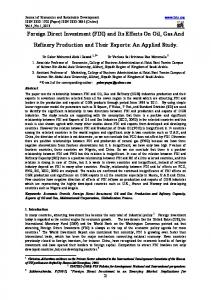
Journal of Economics and Political Economy the FDI in the mining sector, the largest single sub-sector in terms of FDI has been the gold mining industry. As it has been expected, mining contribution to GDP, employment, production and export of minerals have increased. For example, export earnings from mineral export increased from an average of 1 percent of total export in 1997 to 52 percent in 2013 (URT, 2015)2. Similarly, the contribution of mining to the GDP rose from less than 1 percent in 1997 to 3.5 percent in 2013. Also, direct employment in the large scale mining industry increased from 1,700 to 15,000 in 2013. Manufacturing also constitutes a large share of both FDI inflows and stocks. For example, during the 2008-2012 period, FDI inflows and stocks in this sector were, on average, 20 percent and 14 percent of total FDIs (Table 5). The fact that industrial development has been an integral part of Tanzania’s development strategies in the post-independence era (Wangwe et al., 2014), policy makers expected that industrial development would lead the process of transforming the economy from low productivity and low growth to high productivity and dynamic economy (Wangwe et al., 2014) which would in turn generate sustainable growth and reduce poverty. Noteworthy, 53 percent of the industrial structure in the economy is manufacturing. Processing and assembling industries constitute 43 percent and 4 percent respectively. The manufacturing sector in Tanzania consists mainly of food processing, textiles and clothing and chemicals. Other manufacturing industries in the country include basic metal works, non-metallic mineral products, fabricated metal products, beverages, leather and leather products, paper and paper products, publishing and printing, and plastics. The sector has been transformed over time, reflecting changes in national policies, varying domestic demand and the world market dynamics. For example, the Government of Tanzania introduced Sustainable Industrial Development Policy (SIDP) in 1996 to phase itself out of investing directly in productive activities and let the private sector take that role so that the country becomes semi-industrialized by 2025. Indeed, following SIDP in 1996, manufacturing value addition rose tremendously and sustainably (Figure 2). However, the sector value added as a percent of GDP averages at 8 percent over the 1970-2015 period. Also, its growth rate has remained relatively low over the past 4 decades. Notwithstanding, the contribution of manufacturing to GDP must be at a minimum of 40 percent of the GDP in order for Tanzania to become a semiindustrialized country.
2
Gold exports increased from less than 1 tonne in 1997 to 50 tonnes in 2013 (Ministry of Energy and Minerals, 2016).
JEPE, 3(4), M. Epaphra, p.670-719.
677 677
0.4 1.4
Education
Other service activities
21.1
35.9
-23.5
14.9
-0.8 1813.2
953
1.6
0.3 1.4
4
213
3.9
0.5
1.5
22.9
29
1.5
36.9
290.5
2.1 -16.9
83.5
185
95.5
157.1
215
95.9
909.9
2010
385
2009
Source. Tanzania Investment Report, (2013)
1356
2.7
Transportation & storage
ALL
-0.7
26.5
Real estate activities
Professional activities
-3.7
1
Electricity & gas
Construction
127.6
Information & Communication
21.2
81.7
Finance & insurance
Agriculture
129.7
Accommodation
21.1
277.6
Manufacturing
Wholesale & retail trade
669.8
Mining & quarrying
2008
Inflows
1229.6
1.1
1.8
10.4
6.1
12
30.7
31.4
114.5
209.4
-98.3
121.1
165.6
217.3
406.5
2011
2012
1799.5
3.9
0.5
-1
20.1
23.4
-28.1
11.2
-35.2
618.3
-420.1
148.1
5.4
563.7
889.3
Table 5. Flows and Stocks of FDI by Activity (US$ Million), 2008-2012
1430.36
1.4
0.92
4
47.8
12.98
-1.94
23.14
24.08
224.26
-24.44
108.46
71.54
286.04
652.12
20082012
100
0.1
0.1
0.3
3.3
0.9
-0.1
1.6
1.7
15.7
-1.7
7.6
5
20
45.6
%
6756.1
3.8
2
28.8
1.1
79.7
119.5
202.3
372
24.7
532.4
416.3
388.7
870.7
3714.1
2008
7709.2
5.2
2.3
32.7
1.6
81.2
134.4
231.3
355.1
26.8
717.4
512.2
424.6
1085.2
4099.2
2009
9522.5
4.4
3.9
36.7
214.6
82.8
110.9
254.2
392
317.3
801
607.6
445.7
1242.3
5009.1
2010
10752
5.5
5.7
47.1
220.6
94.7
141.5
285.6
506.5
526.7
702.7
728.7
611.3
1459.5
5415.5
2011
Stocks
12551
9.4
6.2
46.1
240.7
118.1
113.4
296.8
471.3
1145
282.6
876.8
616.8
2023.3
6304.8
2012
9458.14
5.66
4.02
38.28
135.72
91.3
123.94
254.04
419.38
408.1
607.22
628.32
497.42
1336.2
4908.54
20082012
100
0.1
0
0.4
1.4
1
1.3
2.7
4.4
4.3
6.4
6.6
5.3
14.1
51.9
%
Journal of Economics and Political Economy
JEPE, 3(4), M. Epaphra, p.670-719.
678 678
Journal of Economics and Political Economy The sector faces a number of challenges including one, low levels of technology, irregular electricity and lack of skilled labour, two, a complex legal and institutional environment where laws are not enforced, three, limited access to financing and high cost of capital, inputs and energy, four, competition from imports, especially very cheap low- quality goods and five, official regulations, charges and taxes (Wangwe et al., 2014).
Figure 2. Manufacturing Value Addition, 1970-2010 Source: Computed using data from UN Statistics Division (2015)
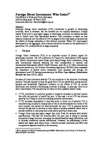
FDI inflows are expected to provide the capital for the desired growth of manufacturing sector. Manufacturing FDI in Tanzania is mainly market- seeking, aimed at penetrating the local or regional markets. Green field investment, merger and acquisitions are the major entry modes of FDI inflows in manufacturing sector in Tanzania. Figure 3 presents the Greenfield manufacturing FDI inflows by subsector, over the 2003-2014 period. Also, Figure 4 reports the top sectors in manufacturing FDI for job creation Greenfield projects (as percent of total) over the same period. Non-metallic mineral products (including buildings and construction matrials) and food, beverage and tobacco had the largest shares of the Greenfield manufacturing FDI inflows. These shares are also reflected in the manufacturing FDI for job creation Greenfield projects. Despite the improvement in manufacturing and mining sectors, agriculture is of critical importance to Tanzania. As stated earlier, the sector accounts for more than 70 percent of total employment but its total valued added is around 30 percent of GDP and its productivity is very low. Also, it makes up for about 17 percent of national export earnings (URT, 2012). Export earnings and employment aside, the need to develop agriculture sector is of paramount importance because of its contribution to food production, poverty reduction and industrial raw materials.
JEPE, 3(4), M. Epaphra, p.670-719.
679 679
Manufacturing Sub-sector
Journal of Economics and Political Economy Non-metallic mineral products (including buildings and construction materials)
791 440
Food, beverages and tobacco
214
Metals and metal products
179
Chemicals and phamaceuticals
61
Motor vehicles and other transport equipements FDI (USD Million)
0
100 200 300 400 500 600 700 800 900
Figure 3. Greenfield Manufacturing FDI Inflows by Sub-sector, 2003-2014, USD Million
Figure 4. Top sectors in Manufacturing FDI for Job Creation Greenfield Projects, 20032014 Percent of Total
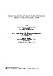
Turning to the agriculture sector, during the last two decades the growth of agriculture sector has been disappointing. The share of agriculture sector in GDP was 49 percent in 1970, 46 percent in 2002 and 26.5 percent in 2007 (Ministry of Agriculture, Food Security and Cooperatives, 2009). The fact that the overall GDP growth has been improving, decline in agriculture implies improvement in the growth in other sectors such as services, manufacturing and mining. It also suggests that the economy moves away from a subsistence economy. As a result, the growth of agriculture sector has been below real GDP growth rate over the last 2 decades (Figure 5). Indeed, the correlation between agriculture-to-GDP ratio and per capita GDP seems to be negative (Figure 6). Also, despite the fact that more than 80 percent of the poor population lives in rural areas and almost all of them rely on subsistence agriculture, valued added-to-GDP ratio has declined constantly during the last 2 decades while population has tremendously increased. This inverse relationship between agriculture value added and number of population, especially during the 1990-2015 period, is reported in Figure 7. In fact, around 10 million of this population is in poverty and 3.4 million is in extreme poverty, compared to respectively less than 1.9 million and 750,000 people who live in poverty and extreme poverty in the urban sector (World Bank Group, 2014). Although agriculture sector has been given priority to reduced poverty, the sector faces many challenges. Many farm sizes are very small because of lack of JEPE, 3(4), M. Epaphra, p.670-719.
680 680
Journal of Economics and Political Economy finance and farming education. Also, factors such as lack of farming technology and climate change adversely affect the living standards of most of population which in turn increase unemployment, hunger and malnutrition. Low production apart, an increase in competition in the world market and shocks in commodity prices have reduced export of main cash crops (Figure 8), which in turn has led to further low production and increase in trade deficit. Thus, the overall positive economic growth experienced in the recent years is not driven by agricultural growth, and certainly not by small-scale farming.
Agriculture, Hunting, Forestry & Fishing (ISIC A-B), Percent of GDP
Figure 5. Agriculture and Real GDP Growth, 1970-2015 40 35 30 25 20 15 10 5 0
y = -0.012x + 34.54 R² = 0.707
0
200
400
600
800
1.000
1.200
Per capita GDP (USD) Figure 6. Correlation between Per Capita GDP and Agriculture, Percent of GDP, 19702015 Source: Computed Using World Bank, WDI Data (2016)
JEPE, 3(4), M. Epaphra, p.670-719.
681 681
Journal of Economics and Political Economy
Figure 7. Agriculture Value Added and Population, 1970-2015 Source: Computed using data from UN Statistics Division (2015) and World Bank, WDI Data (2016)
Figure 8. Export Value Base Quantity: Total Agriculture Products
With fertile soils and considerable water resources, the country provides conditions very well suited to the production of cash crops such as coffee, sisal, tobacco, tea, cotton, cashew nuts and pyrethrum and food crops such as maize, sorghum, millet, rice, wheat, beans, cassava and bananas for ensuring food security. Unfortunately, the sector has not been adequately supported in the past and has not yet performed to its full potential. According to the Ministry of Agriculture, Food Security and Cooperatives (2009), approximately 3.5 million farm families cultivate about 4.5 million hectares of arable land. Crop yields are only 20 percent to 40 percent of their potential. Given the climate change and an increasing global warming, the country has a potential for attaining sustainable irrigation development in order to assure basic food security, improve national standards of living and also contribute to the economic growth of the country. The country has 29.4 million hectares of land suitable for irrigation. Out of these 2.3 million hectares have a high development potential, 4.8 million hectares medium and 22.3 million hectares low irrigation development potential (Ministry of Agriculture, Food Security and Cooperatives, 2009). Nevertheless, financial constraints and the lack of access to financial services limit the ability of small farmers to make the necessary investments and to cover recurrent costs that are associated with modern food supply chains (Reardon JEPE, 3(4), M. Epaphra, p.670-719.
682 682
Journal of Economics and Political Economy & Gulati, 2008) despite the initiatives to provide subsidized inputs and credit and public extension services. Overall, the low average productivity of most small-scale farmers in Tanzania and other Sub-Saharan African countries reveals that small-scale farmers are often unable to overcome the above-mentioned constraints to farming more efficiently, despite the systematic promotion of the smallholder model in the past decades (Collier & Dercon, 2009). Increasing FDI is one important factor contributing to the ongoing transformation of the agricultural sector. FDI in the agricultural sector could contribute to increasing global food supply within a relatively short time and thus contribute to reducing the risks of future food shortages and price hikes (Schüpbach, 2014). FDI may reduce this yield gap by providing financial capital and introducing advanced agricultural technologies as well as the needed skills to employ them efficiently (UNCTAD 2009). Local producers may gain access to modern technologies and management techniques, either through direct cooperation with foreign companies (e.g. as contract farmers) or indirectly through spillovers effects (UNCTAD 2009, p. 160). Also, as Schüpbach (2014) reveals, increased competition may lead local firms to increase their efficiency in order to remain competitive. Admittedly, planned expenditure is biased toward inputs and, recently, rural finance; few resources go to rural infrastructure, value addition, research, and extension. Irrigation expenditure has recently increased but remains insufficient to fill the gap in demand. Rural roads, which are critical for increased agriculture production and productivity, remain significantly underfunded. The total actual public spending on agriculture sector has grown at a slower pace. It increased by 30 percent from 2006/07 to 2010/11 reaching TZS 728 billion (FAO, 2013). In relative terms, however, the agricultural budget allocations have declined from almost 13 percent of total government spending in 2006/07 to about 9 percent in 2010/11 (FAO, 2013). Actual spending in relative terms has also decreased significantly in the same period. The highest share of agriculture sector expenditures in the total budget expenditures fell in the 2007/2008 financial year, both in terms of budget allocations and actual spending, reaching 15 and 17 percent respectively. The importance of agriculture in the total government expenditures has been constantly decreasing (FAO, 2013). Moreover, the analysis shows that large share agricultural sector expenditures goes into current spending, not into capital expenditure, which is critical for creating preconditions for long-term growth. Nevertheless, Tanzania’s own capacity to fill financial gap is limited. Given the limitations of alternative sources of investment finance, foreign direct investment in developing country agriculture could make a significant contribution to bridging the investment gap. In 2012 and 2013, the agriculture sector attracted few investors while manufacturing and tourism sectors attracted the largest number of local and foreign investors (Table 6). In 2013 for example, agriculture sector had only 12 approved foreign projects while manufacturing and tourism sectors, respectively, had 75 and 38 approved foreign projects. In 2012 and 2013, agriculture sector attracted 103 total projects worth TZS 1351 million with employment potentials of 72,574 people while manufacturing sector attracted 550 approved projects worth TZS 5319.80 million with employment potentials of only 50,966 people. JEPE, 3(4), M. Epaphra, p.670-719.
683 683
15 2 7 4 33 7 7 6
Services
Computer
Financial
Communication
Human Resources
Energy
Economic Infrastructure
Broadcasting 718
6
6
7
29
2
4
0
15
139
113
1
184
51 0 161
B
151
0
1
0
4
2
3
2
0
24
15
0
41
9 2 48
C
469
5
5
2
20
2
3
1
1
92
78
0
86
28 2 144
D
205
0
1
2
4
0
2
0
7
35
30
0
74
19 0 31
E
195
1
1
3
9
2
2
1
7
36
20
1
65
13 0 34
F
174,412
127
2,901
4,529
1,781
803
755
67
1,892
17,076
57,541
64
24,039
51,939 110 10,788
G
11,420.10
4.5
261.5
1,344.10
95
2,969.70
67.1
7
424.3
855
838.9
8.1
2,976.40
821.8 5.6 741.2
H
885
7
7
8
32
9
4
1
8
182
132
2
258
43 6 186
A
749
7
6
6
27
8
4
1
5
149
120
2
225
31 5 153
B
136
-
1
2
5
1
-
-
3
33
12
-
33
12 1 33
C
2013
417
5
2
4
14
1
1
-
1
107
77
-
95
15 2 93
D
184
1
-
-
5
2
-
1
3
24
20
-
75
12 3 38
E
284
1
5
5
13
5
3
-
4
51
35
2
88
16 1 55
F
2,593
2,813
2,244
6,979
50
570
16,473
9130
98
26,927
20,635 2,526 10,745
G
202,487
335
100,369
A : Total number of approved projects; B: New projects C: Old projects (expansion and rehabilitation); D: Local projects; E: Foreign Projects; F: Joint projects; G: Total employment; H: Total investment (TZS Million) Source: Tanzania Investment Centre (TIC) and National Bureau of Statistics (NBS), Statistical Abstract, 2013
869
163
Transport
Total
128
Commercial Buildings
1
225
Manufacturing
Petroleum products &Mining
60 2 209
Agriculture and Livestock Natural Resources Tourism
A
2012
Table 6. Approved Projects, 2012 and 2013
88,236.30
31.3
80,035.10
823.1
177.2
944.7
9.9
1.9
29.9
842.4
1,728.00
2.6
2,343.40
529.2 73.3 664.3
H
Journal of Economics and Political Economy
JEPE, 3(4), M. Epaphra, p.670-719.
684 684
8.9 4.1 15.4 9.6 27.4
Manufacturing
Construction
Wholesale, retail, hotels
Transport, storage, communications
Other 100
29.4
8.5
13.3
5.3
8.1
3.8
31.6
2000
100
29.4
8.1
11.8
8.3
7.5
4.9
30
2005
100
25.5
9
12.7
7.6
7.3
5.9
32
2010
100
24.5
6.8
12.6
9.7
7.2
5.8
33.5
2013
100
6.8
0.9
9.8
0.8
2.1
0.9
78.7
1991
100
7.2
0.7
10.1
0.8
1.5
0.3
79.4
2000
100
7.9
1.2
10.7
1.1
2.5
0.5
76
2005
100
8.7
1.5
11.5
1.3
3.2
0.7
73
2010
100
9.4
1.7
12.2
1.4
3.3
0.7
71.3
2013
Employment by Sector (%)
1
4.6
7.4
1.2
6.5
3.6
3.2
0.4
1991
1
4
11.3
1.2
8.1
4.8
12.8
0.4
2000
1
3.7
7
1.1
7.2
3
9.2
0.4
2005
1
3.2
6.4
1.1
6.5
2.6
6.9
0.4
2010
Relative Productivity Levels
Notes: Derived by calculating labour productivity levels (gross value added at constant prices divided by number of persons employed per sector) and by expressing the result as a ratio of total economy labour productivity.
100
2.4
Mining & utilities
Total
32.2
1991
Gross Value Added (current US$, %)
Agriculture
Economic activity
Table 7. GDP, Employment and Relative Productivity Levels, Tanzania, 1991–2013
1
3
6.3
1
7.5
2.5
6.4
0.4
2013
Journal of Economics and Political Economy
JEPE, 3(4), M. Epaphra, p.670-719.
685 685
Journal of Economics and Political Economy Despite the fact that FDI is seen as potentially providing developmental benefits through for example technology transfer and employment creation, the financial benefits to FDI to the economy of Tanzania is a matter of empirical research. In fact, how far FDIs go towards filling the investment gap is uncertain. The low levels of investment in agriculture have led to a decline in agriculture’s share in total economy. Also, the importance of agriculture employment slowly declines reflecting a process of economic diversification from agriculture to new economic sectors and more urbanization. Nonetheless, agriculture remains the mainstay of the economy because of the sizeable share of the labour force engaged in the sector and its important role in the economy (Table 7). Although the mining and manufacturing sectors have registered important real growth rates in recent years, growth is forthcoming from a low base and both sectors still have relatively small shares of overall GDP. FDI and investment distribution in other sectors is as reported in Tables 5 & 6. On average, electricity & gas, and services such as accommodation, finance & insurance, wholesale & retail trade and professional activities constitute a substantial proportion of FDI inflows and stocks. Service sector also constitutes the largest share in GDP. However, in view of rapid population growth, food security and the rising urbanization, significant improvements are required in productivity growth in agriculture in order to increase agricultural output through technological innovations and efficiency. Since over 70 percent of the population in Tanzania lives in rural areas and agriculture is the mainstay of their living, any strategies to address poverty must involve actions to improve agricultural productivity and farm incomes (Msuya, 2007). This also implies that the flow of FDI into agriculture in Tanzania is very important and central to increased productivity and poverty reduction. The correlations between FDI and per capita GDP and selected sectors of the economy are reported in Figures 9-12.
Figure 9. Correlation between FDI and Real GDP, 1970-2015
JEPE, 3(4), M. Epaphra, p.670-719.
686 686
Journal of Economics and Political Economy
Figure 10. Correlation between FDI and Agriculture, 1970-2015
Figure 11. Correlation between FDI and Mining, Manufacturing, & Utilities 1970-2015
Figure 12. Correlation between FDI and Construction, 1970-2015
JEPE, 3(4), M. Epaphra, p.670-719.
687 687
Transportation, Storage, Communication (ISIC I), Percent of GDP
Journal of Economics and Political Economy
-1,0
12,0 10,0 8,0 y = 0.131x + 7.853 R² = 0.061
6,0 4,0 2,0 0,0 0,0
1,0
2,0
3,0
4,0
5,0
6,0
7,0
FDI, Net Inflows, Percent of GDP Figure 13: Correlation between FDI and Transportation, Storage & Communication, 1970-2015
3. Econometric Modeling and Data 3.1. Model Specification A framework of analysis to examine the effects of FDI and control variables on selected sectors of the economy namely agriculture, mining, manufacturing, construction and transport, storage & communication is formulated by considering all those factors that can potentially play a meaningful role in the determination of value added-to-GDP ratios of all these sectors. Apart from FDI-to-GDP ratio, sectoral performance is basically determined by factors such as change in the real per capita income (pGDP), gross fixed capital formation (GFCF), trade liberalization or degree of openness (TL), real exchange rate (RER), labour force (Labour) and inflation rate . Also, availability of agricultural land (Land) may affect agricultural sector performance. Specified models for agriculture, mining, manufacturing, construction and transport, storage & communication sectors performance are as follows: Model 1: Agricultural sector
ln Agrt 0 1 ln FDI t 2 ln pGDPt 3 ln Labourt 4 ln GFCFt
5 ln TLt 6 ln RERt 7 t 8 ln Landt u1t Model 2: Mining sector ln Mint 0 1 ln FDI t 2 ln pGDPt 3 ln Labourt 4 ln GFCFt
5 ln TLt 6 ln RERt 7 t u2 t
(1)
(2)
Model 3: Manufacturing sector
ln Mant 0 1 ln FDI t 2 ln pGDPt 3 ln Labourt 4 ln GFCFt
5 ln TLt 6 ln RERt 7 t u3t
(3)
JEPE, 3(4), M. Epaphra, p.670-719.
688 688
Journal of Economics and Political Economy Model 4: Construction sector ln Constt 0 1 ln FDI t 2 ln pGDPt 3 ln Labourt 4 ln TLt
5 ln RERt 6 t u4t
(4)
Model 5: Transportation, storage & communication sector
ln TSCt 0 1 ln FDI t 2 ln pGDPt 3 ln Labourt 4 ln GFCFt
5 ln TLt 6 ln RERt 7 t u5t
(5)
where
0 , 1 , 2 , , 8
0 , 1 , 2 ,, 7 0 , 1 , 2 ,, 7 0 , 1 , 2 , , 6 1 , 1 , 2 , , 7 t 1,....T u
=
parameters to be estimated in the five models
=
the period of time, years
white noise error term, i.e. u t ~ N 0, 2 = the first difference operator The variables appearing in the equations are defined as follows =
Agr
=
Min Man Const TSC
= = = =
FDI pGDP GFCF
= = =
=
TL
=
RER
=
Labour Land
= =
Agriculture, valued added, percent of GDP. Output in the agricultural sector is made up of crops production, animal farm production, forestry, fishing and hunting. Real aggregate valued added of these sub-sectors of agriculture to proxy for the agricultural sector Mining value added, percent of GDP Manufacturing value added, percent of GDP Construction value added, percent of GDP Transportation, storage and communications value added, percent of GDP Foreign direct investment, percent of GDP Per capita GDP (Real GDP growth/Population) Gross fixed capital formation, percent of GDP. GFCF is made up of machinery, plant, purchases of equipment, industrial buildings, construction of railways and roads. Inflation rate, measured as the growth rate of consumer price index as a proxy of macroeconomic stability. Trade liberalization or trade openness, measured as export and import, percent of GDP. Real exchange rate. It is obtained by multiplying the nominal exchange rate by US CPI and divided by domestic CPI. Population growth, annual percent Agricultural land (sq. km)
The log-linear functional forms are adopted to reduce the possibility or severity of heterogeneity and directly obtain sectoral elasticities with respect to regressors. The main hypothesis for the empirical work is that the contribution of FDI inflow to sectoral value added in Tanzania is positive. This can be confirmed or denied JEPE, 3(4), M. Epaphra, p.670-719.
689 689
Journal of Economics and Political Economy based on the estimated individual values of 1 , 1 , 1 , 1 and 1 in the regression analyses. The null hypotheses are H 0 : 1 0 , H 0 : 1 0 , H 0 : 1 0 , H 0 : 1 0 , and H 0 : 1 0 i.e. FDI inflows do not contribute to individual sectoral valued added, while the alternative hypotheses are H1 : 1 0 , H1 : 1 0 , H1 : 1 0 , H1 : 1 0 and H1 : 1 0 . The data for the variables which are included in the estimation models (agriculture, mining, manufacturing, construction and wholesale & retail trade sectors valued added, real per capita GDP, FDI, real exchange rate, trade as a percent of GDP, real exchange rate and inflation rate) are obtained from UN Statistics Division (2016) and World Bank World Development Indicators, UNCTAD, World Investment Report (2015), Bank of Tanzania and Tanzania Investment Centre. The rationale for including the different variables in the models is based on theory and priory information. The main augment is that if FDI inflow increases then it will increase the value added of sectors such as agriculture, mining, manufacturing, construction and transport, storage and communication because FDI leads to advancement of the technology and improvement of managerial skills which ultimately lead to faster real growth rate of sectors of the economy. A number of previous studies have proven this argument. For example, Feldstein (2000) argues that FDI allows the transfer of technology especially in the form of new varieties of capital inputs, which cannot be achieved through financial investment or trade in goods and services. In the same line, Akulava (2010) argues that FDI provides firms and economies not only with financial resources, but also with modern technologies, advanced production facilities, new markets and new methods of administration. However, the impact of FDI on different sectors of the economy is not straight forward. For example, Findlay (1978) and Wang & Bloomstrom (1992) point out that the importance of FDI as a conduit for transferring technology, relates to the inflows of FDI to manufacturing, construction or service sectors rather than to the primary sector (i.e. agriculture and mining sectors). Indeed, Alfaro (2003) suggests that FDI in the primary sector tends to have a negative effect on growth, while investment in manufacturing and service sectors a positive one. In the service sector, the evidence is ambiguous (Alfaro, 2003). Transfers of technology and management know-how, introduction of new processes, and employee training tend to relate to the manufacturing sector rather than the agriculture or mining sectors (UNCTAD, 2001, Alfaro, 2003). Also, there have been a number of studies in the area of FDI and construction and transport, storage & communication sectors. For example, Topku (2010) assesses the response of construction sector to FDI in India. Similarly, Andrew et. al. (2015) examine the co-integration regression analysis of FDI inflow into construction in Nigeria and find a positive and significant causal relationship at 5 percent level. Transportation, storage & communication sector is part of the tertiary sector which is basically services industry. Foreign investors can increase the efficiency of that sector by bringing new knowledge, technologies, making the overall level of services more corresponding to the world standards through the quality improvement and cost lowering (Akulava, 2011). Mathiyazhogan (2005) find a positive effect of FDI inflow on transportation. Also, Akulava (2011) shows a positive impact of FDI on the construction industry, but negative effect on construction materials and communications. However, as transportation, storage JEPE, 3(4), M. Epaphra, p.670-719.
690 690
Journal of Economics and Political Economy and communication sector is capital intensive, it is less competitive in comparison to manufacturing, hence, there is a possibility that the domestic firms may be crowded out by foreigners (Akulava, 2011). Besides, according to Tondl & Fornero (2008), a positive effect of FDI on transportation and telecommunication sector productivity depends on the income level of the country. By and large, single country studies for example Adhikary (2011) for Bangladesh, Nuzhart (2009) for Pakistan, Hong &Sun (2007) for China and Anuwar &Nguyen (2009) for Vietnam suggest that FDI has a positive and significant effect on sectoral productivity. It is noteworthy that the complexity of the effect of FDI on different sectors of the economy means that there may be trade-offs between different benefits. For instance, Kabelwa (2006) argues that countries may have to choose between investments that offer short as opposed to long-term benefits; the former may lead to static gains but not necessarily to dynamic ones. The mixed effect of FDI on different sectors of the economy has been reported in many studies (Aitken & Harrison, 1999; Katrina et al., 2004; Blomsrtom et al., 1992, Caves, 1974). Thus, even though there is an obvious need in FDI for the economy, it is not clear enough, whether FDI has only a positive effect on all sectors of the Tanzanian economy and what sectors benefit and subsequently lead to economic growth. Since FDI attraction might be costly for the particular sector, it is significant to examine the causal relationship between FDI and different sectors of the economy. Per capita income may affect economic sectors in different ways. Studies show that as per capita incomes rise, the share of agricultural expenditure in total expenditure declines and the share of expenditure on manufactured goods increase (Singariya & Sinha, 2015). This implies that per capita GDP is positively correlated with share of manufacturing sector while there is negative correlation between per capita GDP and value added share of agriculture sector in GDP. Singariya & Sinha (2015) find that the sign of the estimated coefficient in respect of the agriculture and manufacturing sectors are negative and positive respectively, which suggest that the share of agriculture sector and per capita GDP move in opposite direction while the positive coefficient for the share of manufacturing sector suggests that the share of manufacturing sector and per capita GDP move in same direction. According to Anderson (1987), the relative decline of agriculture is clear from both cross-sectional and time-series data. Moreover, in the literature, the nature of the relationship between the construction sector and per capita income is mixed. Also, according to Strassman (1970) construction sector, like agriculture or manufacturing, follows a pattern of change that reflects a country’s level of development. After lagging in early development, construction accelerates in middle-income countries and then falls off. The reason for the inverted U-shaped curve lies in the fact that in the later stages of development there will be less population growth and migration into urban areas making less demand on housing (Anderson, 1987). At the same time there will already be in place a large stock of physical capital in the construction sector itself (Anderson, 1987). In a similar paper, Turin (1978) argues that, to the extent that economic growth is linked to the level and efficiency of capital formation, an association between construction investment and growth is not surprising given that construction output accounts for about 50 per cent of gross fixed capital formation in most countries. Nevertheless, Qifa (2013), using a confidence of 95 percent and smaller than the given significance level of 0.05 , suggests that a highly significant linear relationship JEPE, 3(4), M. Epaphra, p.670-719.
691 691
Journal of Economics and Political Economy exists between real GDP and construction value added in China and China. Also, the scatter diagrams reveal a significant linear relationship between real GDP and construction value added. However, the Bon curve suggests that the relationship between the share of construction in output and economic development is inverted U-shaped (Qifa, 2013). Furthermore, the level of development is related at improving both quantitative and qualitative infrastructure such transport, storage & communications. Similarly, trade liberalization or openness of the economy is intended to promote productivity by exploiting comparative advantages that can be gained through exposure to foreign competition, enhanced technical development and access to economies of scale (Jayanthakumaran, 2002). Trade liberalization has become popular economic policy of both developed and developing countries. Liberalization may lead to efficient allocation of domestic resources which in turn reduces the production of import substitutes and increase production of exportable products which finally increases total output of agriculture, mining, manufacturing, and services sectors. In the same vein, the increase in exports and adjusting for efficient resource allocation may generate comparative advantages which eventually can result a higher producer surplus from the agricultural sector (De Silva, et. al., 2013). According to Hassine, et al., (2010), opening up foreign trade promotes productivity of agriculture. Trade liberalization may allow domestic firms access to cheaper and better technology and better quality inputs and managerial skills from abroad (Miller & Upadhyay, 2000, Baily & Gersbach 1995). The empirical study by De Silva et al., (2013) suggests that the trade openness is positively related to agricultural sector growth, whereas Yan et al., (2011) suggest that openness policy has a strong positive effect on total factor productivity growth, efficiency improvement and technological progress in construction sector. Trade liberalization may allow countries to import the R & D carried out by others because technical progress embodied in new materials, intermediate manufactured products, capital equipment are traded on international markets. In manufacturing sector, previous studies show that trade liberalization has a positive and significant impact on total factor productivity of the sector (Ousmanou & John, 2007; Mahadevan, 2002; Jonsson & Subramaniam, 2001, Anderson, 2001). Greater exposure to international competition generally has a beneficial effect in industry (Forountan, 1991). Nonetheless, the nature of the relationship between trade policy and various sector of the economy remains very much an open question. Empirical studies provide conflicting results. Harris & Kherfi (2001) shows that trade openness has no significant effect on the rate of productivity growth in manufacturing while Adhikary (2011) finds that the degree of trade openness has a negatively affect on total factor productivity of manufacturing. Moreover, globalization may give negative effect on the construction sector through low quality of inputs, for example, low skills foreign workers which subsequently affect the output quality (Ismail et al., 2012) Also, inflation is one of the main variables in the growth of any sector. Costpush and demand-pull inflation are two sources of inflation (Lipsey & Chrystal 2003). In a country when there is demand-pull inflation, due to increasing demand for food, producers are expected to invest more in the agricultural sector, resulting in an increased production which in turn lead to an increase in agriculture to GDP ratio (De Sormeaux & Pemberton, 2011). Indeed, Chaudhry et al., (2013) suggest JEPE, 3(4), M. Epaphra, p.670-719.
692 692
Journal of Economics and Political Economy that inflation and agriculture sector growth are positively and significantly related, and that very low level of inflation in the economy may not be beneficial to the growth of agriculture and services sectors. However, there is no consensus over the point after which the inflation is harmful to growth of the economy. Studies differ substantially across the countries (Epaphra, 2016, Chaudhry et al., 2013). In an opposite view, when there is cost-push inflation, mainly because of a decrease in aggregate agricultural supply, which may be caused by either an increase in wages or an increase in the prices of raw materials, the costs of agricultural production will increase, which in turn lead to a decline in the ratio of agriculture to GDP (De Sormeaux & Pemberton, 2011). By and large, the effect of inflation on sectoral output differs substantially according to the nature of the sector. For example, Chaudhry et al., (2013) find that inflation is harmful to the manufacturing sector growth; whereas, the effect of inflation on services sector growth is positive and statistically significant. However, inflationary increase in the price of construction materials has been one of the major banes to development and a contributing factor to frequent cost overruns and subsequently project abandonment (Oghenekevwe, et al., 2014 and Kaming et. al., 1997). The construction sector is vulnerable to inflation in prices of materials since construction projects involve extensive use of materials (Obiegbu, 2003). In fact, inflation can cause serious problems in the economic accruals or rate of return to constructors for works undertaken, thus loss of profit (Oyediran, 2006). In, the transportation, storage and communication sector, high inflation has a direct and adverse effect on the service providers and their customers’ incomes, leading to a more difficult production and demand environment. This in turn reduces the ratio of transportation, storage & communication value added-to-GDP. For example, as the price of fuel increases and energy cost also moves up, variable cost structure increases. Increase in cost of production and decline demand following increase in price of services may reduce productivity. Next in the list of control variables is real exchange rate. Exchange rate of a country plays a key role in international economic transactions. For example an increase in exchange rate may increase the demand of domestic products and the cost of imported capital and other imported inputs. If a firm is more dependent on imported inputs, there will be more variable costs and less marginal value of capital (Lotfalipour et al., 2013). This suggests that a depreciation of exchange rate causes a reduction in the level of industrial investment. Contrary, there will be an increase in price competitiveness following an exchange rate appreciation (Lotfalipour et al., 2013). Indeed, those sectors, in which output price is determined in the world markets, are likely to be more sensitive to exchange rate movements. However, the effect of currency valuation changes on sectors that rely on export and imported inputs could be either positive or negative (Lotfalipour et al., 2013). A depreciation of the home currency gives domestic industries a cost advantage and their sales will rise (Krugman, 1979, Fung, 2008). According to Fung & Liu (2009), the direction and magnitude of changes in exports and domestic sales affect not only total sales but also productivity and investment. Nonetheless, empirical studies suggest mixed augments, for example, Kandilov & Leblebicioğlu (2011) find a negative effect of exchange rate fluctuations on the industrial sector whereas Fung & Liu (2009) show that the real depreciation lead to an increase in exports, domestic sales, total sales, value-added, and productivity. In addition, Harchaoui, et al., (2005) suggest that the exchange rate changes have no JEPE, 3(4), M. Epaphra, p.670-719.
693 693
Journal of Economics and Political Economy impact on industries investment. Exchange rate may also affect input prices. Likewise, commodity prices tend to be affected by a change in exchange rate (Longmire & Morey, 1983). Also, theories and empirical studies show that factors such population growth rate or labour and gross fixed capital formation can affect the performance of a particular sector and the economy in general. For example, if a country experiences high population growth and therefore has a larger population base, then it can transfer labour to the expanding modern sectors, without reducing the agricultural labour supply (De Sormeaux & Pemberton, 2011). In this case, both the agricultural and modern sector may expand. In fact, population growth could therefore allow the rural sector to play a role in fostering economic growth (Pemberton, 2002). However, increasing population may also adversely affect agriculture-to-GDP ratio, because high population growth may result into pressures on agricultural production expansion leading into land degradation, which in turn lower land productivity (Pender, 1999). This also suggests that availability of agricultural land may lead to an increase in the ratio of agriculture valued addedto-GDP. Furthermore, studies show that a country that needs to meet her objective of economic development needs an increase in gross fixed capital formation. In fact, economic development may be measured through building of capital equipment on a sufficient scale to increase productivity in agriculture, mining, plantations and/or industry (Shuaib & Ndidi, 2015). However, capital is required to construct schools, hospitals, roads, railways, research and development and improve standards of living etc (Jhingan, 2006; Ainabor et al., 2014). Like the preceding factors, the effect of gross fixed capital formation on growth or productivity is not conclusive and indeed, it is a matter of empirical research. Some studies for example, Kormendi & Meguire (1985), Barro (1991), Levine & Renalt (1992) show that the rate of physical capital formation leads to growth, whiles other studies for example, Kendrick (1993) suggests that the capital formation alone does not lead to economic prosperity, rather the efficiency in allocating capital from less productive to more productive sectors influences growth. In summary, it is noteworthy that the empirical literature on the linkage between FDI, level of development, trade liberalization or openness, population growth, gross fixed capital formation, real exchange rate and the rate of inflation and the sectoral performance does not provide a consensus. Some studies document positive effect of these variables on productivity and growth of sectors of the economy while others either report negative relationship or report weak relationship. Besides, the country specific characteristics with respect to the economical, technological, infrastructural and institutional developments indeed matter a lot to gauze empirical relationship (Adhikary, 2011). The present paper thus is of very significant and therefore, it extends a country specific analysis to add knowledge in the empirical literature.
3.2. Estimation Techniques The ordinary least squares method (OLS) is used for estimation. OLS is simple and widely used in empirical work. If the model’s error term is normally, independently and identically distributed (n.i.i.d.), OLS yields the most efficient unbiased estimators for the model’s coefficients, i.e. no other technique can produce unbiased slope parameter estimators with lower standard errors (Ramírez et al., 2002). The co-integration and error-correction methodology (ECM) is
JEPE, 3(4), M. Epaphra, p.670-719.
694 694
Journal of Economics and Political Economy employed. The ECM helps minimizing the possibility of estimating spurious relations, while at the same time retaining long-run information in the data.
3.3. Nature of Data 3.3.1. Descriptive Statistics and Correlation Time series data spanning from 1970 to 2015 are collected and analyzed empirically to determine the effect of FDI and other control variables on various sectors of the economy. In order to ensure trustworthiness of the data and estimation model, appropriate criteria for quantitative time series research such as normality distribution, matrix correlation and multicollinearity are employed and discussed. Tables 8 and 9 provide a descriptive statistics and correlations of the variables included in the model. Since, the calculation of p-values for hypothesis testing is based on the assumption that the population distribution is normal, test for normality assumption is vital. To this end, the Jarque-Bera (JB) statistic is applied to test for normal distribution of the series. This test is based on the sample skewness and sample kurtosis. In the JB test, the null and alternative hypotheses are set as follows: H0: The variable is normally distributed. H1: The variable is not normally distributed. The test statistic is T 2 K 3 S 6 4
2
JB
(6)
with S, K, and T denoting the sample skewness, the sample kurtosis, and the sample size, respectively. Jarque-Bera statistics follows chi-square distribution with two degrees of freedom for large sample. The null hypothesis is rejected if the p-value level of significance, or if the JB 2 2 As reported in Table 8, the descriptive statistics suggest that, the agriculture value added, mining value added, manufacturing value added, construction value added, transportation, storage & communication, gross fixed capital formation, trade liberalization, real exchange rate, the rate of inflation and agricultural land are approximately normally distributed because their respective skewness is close to 0 in absolute values. More significantly, the probabilities of these fail to reject the null hypothesis of normal distribution at 5 percent level of significance. However, both skewness and probabilities of FDI and real per capita GDP reject the null hypothesis of normal distribution. The failure of the normality test is addressed by transforming all variables, except the inflation rate, by using a natural logarithm operator (Stock & Watson, 2003; Murkhejee, White & Wuyts, 2003). The mean is used to measure the central tendency of the variables in the estimated models. The values of the standard deviation which measures the dispersion of the data from their means does not indicate more spread of the data from their means since the values are not larger in relation to the mean values. Likewise, the minimum and maximum values measure the degree of variations in
JEPE, 3(4), M. Epaphra, p.670-719.
695 695
29.6 33.5 22.7 2.9 -0.5 2.5
2.3 0.3
46
Median
Maximum
Minimum
Std. Dev.
Skewness
Kurtosis
JB
Prob.
Obs.
46
0.4
1.9
2.1
0.2
0.9
1.3
4.7
2.5
2.7
Min
46
0.1
6.1
2.2
0.8
1.5
6.4
11.1
7.8
8.1
Man
Source. Author’s computations
29.2
Mean
Agr
46
0.2
3.1
2.4
0.6
2.7
2.2
11.9
5.8
6.1
Cons.
List of regressands
Table 8. Summary of the Values of Variables
46
0.1
3.9
2.0
0.5
0.9
6.6
10.1
7.7
8.1
TSC
46
0
6.5
2.4
0.8
1.8
0.1
5.9
0.3
1.5
FDI
46
0
9.4
3.6
1.1
204.1
179
994
392.2
441.6
pGDP
46
0
9.1
3.4
-1.1
0.2
2.5
3.4
3.1
3.1
Labour
46
0.3
2.5
1.9
-0.2
8.4
11.1
44.2
29.5
27.9
GFCF
List of regressors
46
0.2
2.9
1.8
-0.2
11.3
17.2
56.8
37.5
36.3
TL
46
0.2
3.6
1.7
-0.3
430.9
331.8
1838.1
1210.5
1097
RER
46
0.1
5
1.6
0.4
10.8
3.5
36.1
12.8
16.6
π
46
0.2
2.9
2.4
0.5
33022.7
290000
397000
327500
333441.4
Land
Journal of Economics and Political Economy
JEPE, 3(4), M. Epaphra, p.670-719.
696 696
-0.53
GFCF
0.73
-0.54
0.54
-0.02
-0.07
-0.36
0.43
0.76
-0.15
0.71
-0.48
1
Min
-0.49
-0.27
-0.62
0.42
0.73
0.44
-0.05
0.28
0.77
-0.23
1
Man
0.89
-0.56
0.64
0.55
0.36
0.05
0.64
0.87
0.27
1
Cons.
List of regressands
Source. Authors computations
-0.47
-0.44
Labour
Land
-0.84
pGDP
0.32
-0.46
FDI
π
-0.77
TSC
0.18
-0.49
Cons
RER
-0.42
Man
-0.47
-0.18
Min
TL
1
Agr
Agr
Table 9. Correlation Matrix
-0.05
-0.45
-0.27
0.29
0.72
0.42
0.36
0.24
1
TSC
0.87
-0.56
0.5
0.31
0.17
-0.16
0.69
1
FDI
0.77
-0.25
0.04
0.24
0.18
0.19
1
pGDP
-0.04
0.23
-0.05
0.65
0.53
1
Labour
0.04
-0.51
-0.01
0.82
1
GFCF
List of regressors
0.27
-0.29
0.27
1
TL
0.61
-0.19
1
RER
-0.32
1
Π
1
Land
Journal of Economics and Political Economy
JEPE, 3(4), M. Epaphra, p.670-719.
697 697
Journal of Economics and Political Economy the data. In addition to descriptive statistics, the JB statistics test is used to test for normality of the residuals and the results are reported in the empirical findings section. In the same vein, Table 9 reports the correlation matrix of the variables of the regression model. Surprisingly, agriculture valued added, is negatively correlated with FDI, per capita GDP, labour, gross fixed capital formation and trade liberalization but positively correlated with inflation. In fact, these correlations are matters of empirical study interest. In contrast, and as it is expected, FDI is positively associated with per capita GDP, mining value added, manufacturing value added and construction value added. The correlation matrix also shows that the pair-wise correlations between regressors are not quite high (i.e. less than 0.8), indicating that multicollinearity is not a serious problem.
3.3.2. Unit Root Test Many macroeconomic and financial time series such as exchange rates, real GDP and inflation exhibit stochastic trends or nonstationarity. In fact, they have a tendency not to revert to a mean level, but they wander for prolonged periods in one direction or the other. It is widely documented that trends, either stochastic or deterministic, may cause spurious regressions. This occurs when a non-stationary variable is regressed on a completely unrelated non-stationary variable but yields a reasonably high value of R 2 , apparently indicating that the model fits well. This implies, it is very difficult to perform any hypothesis tests in models which inappropriately use non-stationary data since the test statistics will no longer follow the t or F distributions which are assumed they would, so any inferences which are made are likely to be invalid. Such variables can be made stationary by transforming them into their differences. Stationarity or unit root tests are used to determine if trending data should be first differenced or regressed on deterministic functions of time to render the data stationary. A time series, Yt is said to be stationary if its statistical properties (mean, variance, autocorrelation) do not vary with time. There are two different approaches to unit root or nonstationarity. Tests such as KwiatkowskiPhillips-Schmidt-Shin (KPSS) test, Leybourne & McCabe test consider the null hypothesis that the series is stationary whereas tests such as Dickey-Fuller (DF) test, augmented Dickey-Fuller (ADF) test, Phillips-Perron (PP) test and DF-GLS test consider the null hypothesis that the series is not stationary. This paper uses ADF test. The ADF test makes a parametric correlation for higher-order correlation by assuming that the series follows autoregressive process and adjusting the test methodology. Moreover the ADF approach controls for higher-order correlation by adding lagged difference terms of the dependent variable to the right-hand side of the regression. The basic idea behind the ADF unit root test for nonstationarity is to regress Yt on its lagged value Yt 1 and find out if the estimated is statistically equal to 1 or not in the model
Yt Yt 1 1Yt 1 ut
(7)
Yt Yt 1 ut
JEPE, 3(4), M. Epaphra, p.670-719.
698 698
Journal of Economics and Political Economy
where 1 , and is the first difference operator. Equation (7) is estimated and tested for the null hypothesis of 0 against the alternative of 0 . If 0 , then 1 , there is a unit root problem and the series in equation is said to be nonstationary. In order to make the error term, u t white noise, i.e. u t ∼ NID0, 2 , the lags of the first difference are included in the regression equation. Therefore, the regression equation (7) is presented in the form k
Yt Yt 1 t Yt i ut
(8)
i 1
Also, the intercept as well as a time trend t may be included to form m
Yt 1 2 t Yt 1 t Yt i ut
(9)
i 1
The testing procedure for the ADF unit root test is applied to the model q
yt t yt 1 j yt j uit
(10)
j 1
where is a constant, is the coefficient on a time trend series, is the coefficient of yt 1 , q is the lag order of the autoregressive process, yt y t yt 1 are first differences of y t , yt 1 are lagged values of order one of y t yt j are changes in lagged values, and u it it is the white noise (Ssekuma, 2011). The results of the ADF test are presented in Table 10. ADF Unit root test indicates that the hypothesis of a unit root cannot be rejected in all variables in levels. It is therefore concluded that all variables are non-stationary at their levels. However, the hypothesis of a unit root is rejected in first differences and hence the original series is integrated of order one i.e. I 1 . The unit root test results for the first difference are also reported in Table 10. This also suggests that in order to avoid spurious correlation, further estimations could be carried while in first difference.
3.3.3. Cointegration Test and Error Correction Model Having established that the variables are non stationary at level but when integrated of the same order (i.e. first difference) they become stationary, the next procedure is to test the possibility of long run relationship among the variables used in the regression model. In fact, if there exists a stationary linear combination of nonstationary random variables, the variables combined are said to be cointegrated. Testing for cointegration is, thus, a test for the existence of the equilibrium relationship postulated. Engle & Granger (1987) two-step estimation procedure and the Johansen (1988) procedure are two procedures that are popularly used to identify and estimate the cointegrating vectors and the short run adjustment parameters. The former procedure involves normalizing the cointerating vector on one of the variables, which makes the assumption that the corresponding element JEPE, 3(4), M. Epaphra, p.670-719.
699 699
Journal of Economics and Political Economy of the cointegrating vector is non-zero. The Johansen procedure is a multivariate approach, the estimation of which would consume a lot of degree of freedom. In this paper, the Johansen procedure is used. The Johansen's procedure builds cointegrated variables directly on maximum Table 10. ADF Unit Root Test Levels Constant
Optimal Lag = 1
1 0
Ln(Agr) Ln(Land) Ln(FDI) Ln(pGDP) Ln(Labour) Ln(GFCF) Ln(TL) Ln(RER)
-1.853 0.597 -2.687 -1.287 -1.357 -2.254 -0719 -1.131 -2.016 -2.314 -1.312 -0.784 -0.566
Ln(Min) Ln(Man) Ln(Cons.) Ln(TSC)
5% Critical Value -2.928 Null Hypothesis: there is a unit root Source: Author’s computations
Constant and Trend
First Difference, ∆ Constant Constant & Trend
1 0
1 2 0
-1.230 -2.109 -3.409 -1.749 -2.283 -2.209 -2.528 -1.713 -2.508 -2.286 -0.489 -2.275 -0.329
-7.562 -6.722 -7.653 -4.349 -5.770 -4.585 -4.919 -5.799 -7.568 -7.206 -5.715 -8.130 -7.655
-8.068 -6.77 -7.567 -4.301 -5.887 -4.793 -4.994 -5.729 -7.695 -7.149 -6.118 -8.239 -8.622
-3.513
-2.929
-3.516
1 2 0
Likelihood estimation instead of relying on OLS procedures (Johansen & Juselius, 1988).The main advantage of the Johansen Maximum Likelihood (ML) method is that it enables one to determine the number of existing cointegrating (i.e. long-run) relationships among the variables in hand. It is important to note that single equation-based approaches assume the uniqueness of the cointegrating vector. The Johansen test is performed if all the variables are of the same order of nonstationary, and in fact are I 1 . The variables that are to be tested for cointegration are stacked into a p-dimensional vector y t then a p1 vector of first differences,
yt , is constructed and form and estimate the vector autoregressive model
yt yt k 1yt 1 2 yt 2 k 1yt k 1 ut
(11)
The rank of the matrix is tested. If is of zero rank (i.e. all the eigenvalues are not significantly different from zero), there is no cointegration, otherwise, the rank will give the number of cointegrating vectors (Brooks, 2008). The Johansen and Juselius maximum likelihood test is done on the variables in their nonstationary form and the trace test and maximum eigenvalue test, are as shown in equations (12) and (13) respectively. n
J trace T ln 1 ˆi i r 1
J max T ln 1 ˆr 1
(12) (13) JEPE, 3(4), M. Epaphra, p.670-719.
700 700
Journal of Economics and Political Economy where J trace is the trace statistic, J max is the eigen-max statistc, T is the sample size and ˆi is the ith largest canonical correlation. The trace test tests the null hypothesis of r cointegrating vectors against the alternative hypothesis of n cointegrating vectors whereas the maximum eigenvalue test tests the null hypothesis of r cointegrating vectors against the alternative hypothesis of r 1 cointegrating vector (Hjalmarsson & Österholms, 2007). The results for testing the number of cointegrating relations for the 5 models are reported in Tables 11.1-11.5. The first column is the number of cointegrating relations under the null hypothesis, the second column is the ordered eigenvalues of the matrix, the third column is the test statistic, and the last two columns are the 5 percent critical and probability values. The critical values are taken from MacKinnon-Haug-Michelis (1999). Trace statistic is used to determine the presence of co-integration between variables. On the basis of the trace statistic value test, the null hypothesis of no cointegration r 0 is rejected at the 5 percent level of significance in favour of the specific alternative, namely that there is at most 7 cointegrating vector, 6 cointegrating vector, 5 cointegrating vector, 5 cointegrating vector, and 4 cointegrating vector for model 1, model 2 model 3, model 4 and model 5 respectively3. The implication is that a linear combination of all the series for all models is found to be stationary and that there is a stable longrun relationship between the series. If cointegration is proven to exist, then the next step is to estimate error correction model (ECM) that indicates the speed of adjustment from the short-run equilibrium to the long-run equilibrium state. Indeed, since there is co-integration among dependent variables and its fundamentals, an ECM has to be estimated by incorporating the lagged error correction term, ECM 1 , in the set of regressors (Johansein et al, 2010). The error correction term is the residual from the static long run regression and it joins the set of differenced non-stationary variables to be estimated to capture both short run and long run dynamics. The greater the coefficient of the parameter, the higher the speed of adjustment of the model from the short-run to the long run state will be. Table 11. 1. Johansen Tests for Cointegration Model 1: Series: Agr, FDI , pGDP Labour, GFCF, TL, RER, Hypothesized Trace No. of CE(s) Eigenvalue Statistic None * 0.944926 487.4641 At most 1 * 0.876037 362.8039 At most 2 * 0.848230 273.0298 At most 3 * 0.763553 191.9581 At most 4 * 0.686623 129.9508 At most 5 * 0.577073 80.05574 At most 6 * 0.504724 43.05188 At most 7 0.234636 12.83832 At most 8 0.030682 1.339978 Trace test indicates 7 cointegrating eqn(s) at the 0.05 level * denotes rejection of the hypothesis at the 0.05 level **MacKinnon-Haug-Michelis (1999) p-values 3
and Land 0.05 Critical Value 197.3709 159.5297 125.6154 95.75366 69.81889 47.85613 29.79707 15.49471 3.841466
Prob.** 0.0001 0.0000 0.0000 0.0000 0.0000 0.0000 0.0009 0.1209 0.2470
This is because the first significant value, where trace statistic is less than critical value at 5 percent level, is found at maximum rank of 7, 6, 5, 5, and 4.
JEPE, 3(4), M. Epaphra, p.670-719.
701 701
Journal of Economics and Political Economy Table 11.2. Johansen Tests for Cointegration Model 2: Series: Min, FDI, pGDP, Labour, GFCF, TL, RER, and Hypothesized Trace No. of CE(s) Eigenvalue Statistic None * 0.754196 229.9379 At most 1 * 0.632015 168.1962 At most 2 * 0.565840 124.2089 At most 3 * 0.511048 87.49787 At most 4 * 0.425635 56.01631 At most 5 * 0.342521 31.61877 At most 6 0.258041 13.16770 At most 7 0.000804 0.035387 Trace test indicates 6 cointegrating eqn(s) at the 0.05 level * denotes rejection of the hypothesis at the 0.05 level **MacKinnon-Haug-Michelis (1999) p-values
0.05 Critical Value 159.5297 125.6154 95.75366 69.81889 47.85613 29.79707 15.49471 3.841466
Table 11.3. Johansen Tests for Cointegration Model 3: Series: Man, FDI , pGDP, Labour, GFCF, TL, RER and Hypothesized Trace No. of CE(s) Eigenvalue Statistic None * 0.775949 242.9874 At most 1 * 0.685538 177.1686 At most 2 * 0.610239 126.2653 At most 3 * 0.510811 84.80754 At most 4 * 0.457706 53.34729 At most 5 0.309122 26.42167 At most 6 0.200013 10.15079 At most 7 0.007512 0.331764 Trace test indicates 5 cointegrating eqn(s) at the 0.05 level * denotes rejection of the hypothesis at the 0.05 level **MacKinnon-Haug-Michelis (1999) p-values
Model 4: Series: Cons, FDI, pGDP, Labour, GFCF, TL, RER and Hypothesized No. of CE(s)
None * At most 1 * At most 2 * At most 3 * At most 4 * At most 5 At most 6 At most 7
0.05 Critical Value 159.5297 125.6154 95.75366 69.81889 47.85613 29.79707 15.49471 3.841466
Table 11.4. Johansen Tests for Cointegration
Prob.** 0.0000 0.0000 0.0002 0.0010 0.0071 0.0305 0.1088 0.8507
Prob.** 0.0000 0.0000 0.0001 0.0020 0.0140 0.1166 0.2693 0.5646
Eigenvalue
Trace Statistic
0.05 Critical Value
Prob.**
0.875519 0.617839 0.531377 0.458583 0.435296 0.301857 0.251977 0.002293
248.1794 156.5009 114.1767 80.82659 53.82969 28.68573 12.87514 0.100996
159.5297 125.6154 95.75366 69.81889 47.85613 29.79707 15.49471 3.841466
0.0000 0.0002 0.0015 0.0051 0.0124 0.0667 0.1195 0.7506
Trace test indicates 5 cointegrating eqn(s) at the 0.05 level * denotes rejection of the hypothesis at the 0.05 level **MacKinnon-Haug-Michelis (1999) p-values
JEPE, 3(4), M. Epaphra, p.670-719.
702 702
Journal of Economics and Political Economy Table 11.5. Johansen Tests for Cointegration
Model 5: Series: TSC, FDI, pGD, Labour, GFCF, TL, RER and Hypothesized Trace No. of CE(s) Eigenvalue Statistic None * 0.815332 234.1974 At most 1 * 0.680481 159.8727 At most 2 * 0.526750 109.6714 At most 3 * 0.469332 76.75366 At most 4 * 0.371358 48.87440 At most 5 0.335801 28.44988 At most 6 0.190902 10.44624 At most 7 0.025255 1.125499 Trace test indicates 5 cointegrating eqn(s) at the 0.05 level * denotes rejection of the hypothesis at the 0.05 level **MacKinnon-Haug-Michelis (1999) p-values
0.05 Critical Value 159.5297 125.6154 95.75366 69.81889 47.85613 29.79707 15.49471 3.841466
Prob.** 0.0000 0.0001 0.0039 0.0126 0.0400 0.0709 0.2480 0.2887
4. Empirical Results and Discussions The results of the regression analysis for the five models are reported in Tables 12.1-16.2. The last four models are estimated without land. The Durbin Watson (DW) statistic included in the result is used to test for auto-correlation in the error term. It should be noted that, as a rule of thumb, if DW is found to be 2 in an application one may conclude that there is no first order autocorrelation either positive or negative. Therefore, the closer DW is to 2, the greater the evidence of no serial correlation in the residuals. Also, various diagnostic tests are used to assess the model. These include White Heteroskedasticity test, Breusch-Godfred LM test, ARCH LM test, Ramsey RESET and JB Normality test. The heteroskedasticity test is based on the null hypothesis of heteroskedasticity not present, LM test for autocorrelation up to order 1 is based on the null hypothesis that there is no autocorrelation; test for ARCH of order 1 is based on the null hypothesis that no ARCH effect is present, the Ramsey RESET test for specification is based on the null hypothesis of adequate specification, and test for normality of residuals is based on null hypothesis that the errors are normally distributed. In view of these hypotheses, the regression models pass all specification tests. On the same importance, the F-statistic is significant at 1 percent level in all models, except model 5, rejecting the null hypotheses that the coefficients are equal to zero. Model 5, itself has a significant F-statistic of 5 percent. This implies that the models are significantly explained by the regressors hence acceptable in overall terms. In addition, cumulative sum of recursive residuals (CUSUM) is used to test the stability of the models. In the use of the CUSUM plots, if the statistics stay within the critical bonds of 5 percent level of significance, the null hypothesis of all coefficients in the given regression are stable and cannot be rejected. Understandably the R 2 and adjusted R 2 are relative low, however, low values of R 2 , do not mean that factors in disturbance term are correlated with the independent variables (Wooldridge, 2006). The t values and standard errors are presented to test for the significance of the coefficient estimates. The p-values indicate the level of significance. The results show that, inconsistent with the a priori expectation, the coefficient of FDI in the agricultural sector has a negative sign and statistically significant at 5 percent level. On average, a 1 percent increase in FDI-to-GDP ratio may lead to an average of 0.005 percent decrease in agriculture valued added-to-GDP ratio, holding other factors constant. Indeed, this is a surprising result; however, the inverse causal relationship between FDI and agriculture value added can be JEPE, 3(4), M. Epaphra, p.670-719.
703 703
Journal of Economics and Political Economy attributed to many factors including low flow of FDI in the agricultural sector relative to mining and manufacturing sectors. This is evidenced by relative few approved projects in agriculture sector. Also, poor quality products and the lack of adequate infrastructure results in high energy and transportation costs rendering commodities non-competitive which in turn results into loss of market share. Furthermore, agricultural sector depends on smallholder producers with limited education and experience and are exposed to shock. As a result, the ratio of agriculture value added-to-GDP has been declining despite the fact that FDI-toGDP ratio has been slightly increasing. This also suggests that FDI is still needed in agriculture sector. Some impacts of FDI in the agriculture sector should be measured in knowledge acquisition, technology and international image. As it is expected, the coefficients for the FDI-to-GDP ratio on manufacturing, construction and transport, storage and communication sectors are positive and respectively, statistically significant at 5 percent, 1 percent and 1 percent levels. A 1 percent increase in FDI-to-GDP ratio may lead, on average, to a 0.006 percent increase in manufacturing value added-to-GDP ratio, other factors being equal. In fact, the positive impact of FDI on manufacturing sector is not surprising because the proportion of FDI inflows to this sector is substantial. Also, results suggest that a 1 percent increase in FDI-to-GDP ratio may lead, on average, to a 0.01 percent increase in transport, storage and communication value added-to-GDP ratio. Moreover, FDI seems to have a positive and very strong effect on construction sector in Tanzania. On average, a 1 percent increase in the ratio of FDI-to-GDP may lead to a 0.65 increase in the ratio of construction value added-to-GDP ceteris paribus. This is very important for the economy because construction sector occupies a significant focal point to the process of development. The fact, that FDI is associated with technology advancement, transfer of advanced skills and management, market access and competition improvement, it is anticipated FDI to lead to an increase in value added of manufacturing, construction, and transport, storage and communication sectors. The coefficient of FDI on the mining sector seems to be statistically insignificant. This suggests that FDI exerts no effect on mining value added. The lack of causal relationship between FDI and mining sector, despite the fact that the sector is predominantly dominated by foreign investor is very interesting. However, this result is very similar to that of Rutaihwa & Simwela (2012). In fact, cross-country studies reveal negative relationship of FDI in the growth of primary sector (agriculture and mining) and positive in the secondary sector (manufacturing and construction industry). For example, Khaliq & Noy (2000) reveal a negative effect of FDI on the growth in the mining & quarrying. This mixed results, confirms the findings by Alfaro (2003); Noy & Vu (2007); Aykut & Sayek (2007); Mathiyazhogan (2005); Khaliq & Noy (2006). In particular, Chandana (2008) suggests that growth effects of FDI vary widely across sectors. FDI stocks and output are mutually reinforcing in the manufacturing sector, whereas any causal relationship is absent in the primary sector (Chandana, 2008)
JEPE, 3(4), M. Epaphra, p.670-719.
704 704
Journal of Economics and Political Economy Table 12.1. Empirical Results, Dependent Variable: ∆Ln(Agr) Variable
Coefficient 0.509
C ∆ Ln(Agr)-1 ∆Ln(FDI) ∆Ln(pGDP) ∆Ln(Labour) ∆Ln(GFCF) ∆Ln(TL) ∆Ln(RER) ∆
Std. Error 0.521
-0.223 -0.005** -0.094* 4.066** -0.061* -0.035* 0.011 -0.001 -0.038 -0.020* 0.502 0.346 3.22 0.005
∆Ln(Land) ECM-1 R-squared Adjusted R-squared F-statistic Prob(F-statistic)
t-Statistic 0.976
Prob. 0.336
-0.875 -2.430 -1.941 2.264 -1.911 -1.774 0.358 -1.013 -0.926 -1.836
0.388 0.020 0.061 0.030 0.065 0.085 0.722 0.318 0.360 0.075 1.970
0.255 0.002 0.048 1.796 0.032 0.020 0.030 0.001 0.041 0.011 Durbin-Watson stat
***, **, * show significant at 1, 5 and 10 percent level of significance
Table 12.2. Serial Correlation, Heteroskedasticity and Ramsey RESET Tests Breusch-Godfrey Serial Correlation LM Test: F-statistic 0.052263 Obs*R-squared 0.149299 Heteroskedasticity Test: Breusch-Pagan-Godfrey F-statistic 1.424708 Obs*R-squared 13.24677 Heteroskedasticity Test: ARCH F-statistic 0.028029 Obs*R-squared 0.060395 Ramsey RESET Test Value t-statistic 0.543413 F-statistic 0.295297 Likelihood ratio 0.407667
Prob. F(2,30) Prob. Chi-Square(2)
0.9492 0.9281
Prob. F(10,32) Prob. Chi-Square(10)
0.2143 0.2102
Prob. F(2,38) Prob. Chi-Square(2)
0.9724 0.9703
Probability 0.5907 0.5907 0.5232
Source: Author’s Computation 12
Series: Residuals Sample 1973 2015 Observations 43
10
8
6
4
2
0 -0.04
-0.02
0.00
0.02
Mean Median Maximum Minimum Std. Dev. Skewness Kurtosis
6.62e-18 0.001050 0.049704 -0.035353 0.018117 0.525903 3.270604
Jarque-Bera Probability
2.113314 0.347616
0.04
Figure 12.1. Model1, Normality Test of the Residuals: Histogram Source: Author’s Computation
JEPE, 3(4), M. Epaphra, p.670-719.
705 705
Journal of Economics and Political Economy 20 15 10 5 0 -5 -10 -15 -20 84
86
88
90
92
94
96
98
CUSUM
00
02
04
06
08
10
12
14
5% Significance
Figure 12.2. Model 1, Stability Test: CUSUM Source: Author’s Computation
Table 13.1. Empirical Results, Dependent Variable: ∆Ln(Min) Variable C ∆ Ln(Min)-1 ∆Ln(FDI) ∆Ln(pGDP) ∆Ln(GFCF) ∆Ln(Labour) ∆Ln(TL) ∆Ln(RER) ∆ ECM-1 R-squared Adjusted R-squared F-statistic Prob(F-statistic)
Coefficient 0.006 1.193** 0.004 0.425* 0.362** 0.994 -0.305*** -0.358** 0.001 -1.328*** 0.490 0.350 3.517 0.003
Std. Error t-Statistic 0.282 0.023 0.290 4.106 0.011 0.328 0.219 1.946 0.174 2.077 9.191 0.108 0.111 -2.732 0.158 -2.266 0.002 0.455 0.318 -4.172 Durbin-Watson stat
Prob. 0.982 0.000 0.744 0.060 0.046 0.914 0.010 0.030 0.652 0.000 1.946
***, **, * show significant at 1, 5 and 10 percent level of significance Source: Author’s Computation
Table 13.2. Serial Correlation, Heteroskedasticity and Ramsey RESET Tests Breusch-Godfrey Serial Correlation LM Test: F-statistic 0.912784 Obs*R-squared 2.391411 Heteroskedasticity Test: Breusch-Pagan-Godfrey F-statistic 0.778900 Obs*R-squared 7.533952 Heteroskedasticity Test: ARCH F-statistic 1.175212 Obs*R-squared 2.388263 Ramsey RESET Test Value t-statistic 0.491753 F-statistic 0.241821 Likelihood ratio 0.323726
Prob. F(2,31) Prob. Chi-Square(2)
0.4119 0.3025
Prob. F(9,33) Prob. Chi-Square(9)
0.6368 0.5817
Prob. F(2,38) Prob. Chi-Square(2)
0.3197 0.3030
Probability 0.6263 0.6263 0.5694
Source: Author’s Computations
JEPE, 3(4), M. Epaphra, p.670-719.
706 706
Journal of Economics and Political Economy 6
Series: Residuals Sample 1973 2015 Observations 43
5
4
3
2
1
Mean Median Maximum Minimum Std. Dev. Skewness Kurtosis
-9.04e-18 0.002491 0.189635 -0.292512 0.100872 -0.403359 3.551277
Jarque-Bera Probability
1.710502 0.425176
0 -0.3
-0.2
-0.1
0.0
0.1
0.2
Figure 13.1. Model 2, Normality Test of the Residuals: Histogram Source: Author’s Computation 20 15 10 5 0 -5 -10 -15 -20 84
86
88
90
92
94
96
CUSUM
98
00
02
04
06
08
10
12
14
5% Significance
Figure 13.2. Model 2, Stability Test: CUSUM Source: Author’s Computation Table 14.1. Empirical Results, Dependent Variable: ∆Ln(Man) Variable C ∆ Ln(Man)-1 ∆Ln(FDI) ∆Ln(pGDP) ∆Ln(GFCF) ∆Ln(Labour) ∆Ln(TL) ∆Ln(RER) ∆ ECM-1 R-squared Adjusted R-squared F-statistic Prob(F-statistic)
Coefficient -0.012** 0.327 0.006** 0.176*** 0.115** 0.177 -0.024 0.049 -0.003*** -0.559** 0.565 0.446 4.756 0.000
Std. Error t-Statistic 0.006 -1.986 0.209 1.618 0.003 1.981 0.064 2.754 0.053 2.140 0.189 0.935 0.042 -0.576 0.048 1.022 0.001 -3.472 0.255 -2.178 Durbin-Watson stat
Prob. 0.054 0.115 0.054 0.009 0.039 0.356 0.568 0.314 0.002 0.037 2.108017
***, **, * show significant at 1, 5 and 10 percent level of significance Source: Author’s Computation
JEPE, 3(4), M. Epaphra, p.670-719.
707 707
Journal of Economics and Political Economy Table 14.2. Serial Correlation, Heteroskedasticity and Ramsey RESET Tests Breusch-Godfrey Serial Correlation LM Test: F-statistic 0.997390 Obs*R-squared 2.599671 Heteroskedasticity Test: Breusch-Pagan-Godfrey F-statistic 0.483911 Obs*R-squared 5.013321 Heteroskedasticity Test: ARCH F-statistic 0.016281 Obs*R-squared 0.035103 Ramsey RESET Test Value t-statistic 1.625417 F-statistic 2.641980 Likelihood ratio 3.411204
Prob. F(2,31) Prob. Chi-Square(2)
0.3804 0.2726
Prob. F(9,33) Prob. Chi-Square(9)
0.8748 0.8331
Prob. F(2,38) Prob. Chi-Square(2)
0.9839 0.9826
Probability 0.1139 0.1139 0.0648
Source: Author’s Computation
9
Series: Residuals Sample 1973 2015 Observations 43
8 7 6 5 4 3 2 1
Mean Median Maximum Minimum Std. Dev. Skewness Kurtosis
-1.19e-18 4.22e-05 0.067346 -0.084286 0.028298 -0.480813 4.222348
Jarque-Bera Probability
4.333789 0.114533
0 -0.08
-0.06
-0.04
-0.02
0.00
0.02
0.04
0.06
Figure 14.1. Model 3, Normality Test of the Residuals: Histogram Source: Author’s Computation 20 15 10 5 0 -5 -10 -15 -20 84
86
88
90
92
94
96
CUSUM
98
00
02
04
06
08
10
12
14
5% Significance
Figure 14.2: Model 3, Stability Test: CUSUM Source: Author’s Computation
JEPE, 3(4), M. Epaphra, p.670-719.
708 708
Journal of Economics and Political Economy Table 15.1. Empirical Results, Dependent Variable, ∆Ln(Cons) Variable C ∆ Ln(Cons)-1 ∆Ln(FDI) ∆Ln(pGDP) ∆Ln(Labour) ∆Ln(RER) ∆Ln(TL) ∆ ECM-1 R-squared Adjusted R-squared F-statistic Prob(F-statistic)
Coefficient 0.037* -0.013 0.653*** 0.421** 0.035 -0.258* 0.084 0.006** -0.024** 0.609 0.503 5.722 0.000
Std. Error t-Statistic 0.019 1.905 0.195 -0.066 0.175 3.733 0.208 2.022 0.627 0.056 0.152 -1.700 0.133 0.633 0.003 2.222 0.011 -2.161 Durbin-Watson stat
Prob. 0.065 0.947 0.000 0.051 0.955 0.089 0.531 0.033 0.038 2.051
***, **, * show significant at 1, 5 and 10 percent level of significance Source: Author’s Computation
Table 15.2. Serial Correlation, Heteroskedasticity and Ramsey RESET Tests Breusch-Godfrey Serial Correlation LM Test: F-statistic 1.069894 Obs*R-squared 2.776448 Heteroskedasticity Test: Breusch-Pagan-Godfrey F-statistic 1.584104 Obs*R-squared 12.97266 Heteroskedasticity Test: ARCH F-statistic 0.892834 Obs*R-squared 1.840171 Ramsey RESET Test Value t-statistic 0.122103 F-statistic 0.014909 Likelihood ratio 0.020030
Prob. F(2,31) Prob. Chi-Square(2)
0.3554 0.2495
Prob. F(9,33) Prob. Chi-Square(9)
0.1609 0.1638
Prob. F(2,38) Prob. Chi-Square(2)
0.4179 0.3985
Probability 0.9036 0.9036 0.8875
Source: Author’s Computation 8
Series: Residuals Sample 1973 2015 Observations 43
7 6 5 4 3
Mean Median Maximum Minimum Std. Dev. Skewness Kurtosis
2.58e-18 -0.000594 0.172223 -0.223530 0.095887 -0.108669 2.673276
Jarque-Bera Probability
0.275889 0.871147
2 1 0 -0.20
-0.15
-0.10
-0.05
0.00
0.05
0.10
0.15
Figure 15.1. Model 4, Normality Test of the Residuals: Histogram Source: Author’s computations
JEPE, 3(4), M. Epaphra, p.670-719.
709 709
Journal of Economics and Political Economy 20 15 10 5 0 -5 -10 -15 -20 84
86
88
90
92
94
96
CUSUM
98
00
02
04
06
08
10
12
14
5% Significance
Figure 15.2. Model 4, Stability Test: CUSUM Source: Author’s Computation
Table 16.1. Empirical Results, Dependent Variable ∆Ln(TSC) Variable C ∆ Ln(TSC)-1 ∆Ln (FDI) ∆Ln (pGDP) ∆Ln (GFCF) ∆Ln (Labour) ∆Ln (TL) ∆Ln(RER) ∆ ECM-1 R-squared Adjusted R-squared F-statistic Prob(F-statistic)
Coefficient 0.012 -0.646** 0.011*** 0.011 0.054 -0.008 0.089* -0.065 -0.001 -0.064 0.387461 0.220405 2.319350 0.037848
Std. Error t-Statistic 0.007 1.673 0.289 -2.236 0.003 3.711 0.072 0.159 0.054 1.010 0.223 -0.038 0.049 1.827 0.057 -1.134 0.001 -0.358 0.024 -2.624 Durbin-Watson stat
Prob. 0.103 0.032 0.001 0.875 0.310 0.970 0.076 0.265 0.722 0.0128 2.006436
***, **, * show significant at 1, 5 and 10 percent level of significance Source: Author’s Computation
Table 16.2. Serial Correlation, Heteroskedasticity and Ramsey RESET Tests BreuschGodfrey Serial Correlation LM Test: F-statistic 0.125124 Obs*R-squared 0.344339 Heteroskedasticity Test: Breusch-Pagan-Godfrey F-statistic 0.930346 Obs*R-squared 8.702363 Scaled explained SS 5.047840 Heteroskedasticity Test: ARCH F-statistic 1.616457 Obs*R-squared 11.62571 Ramsey RESET Test Value F-statistic 1.505043 Likelihood ratio 12.40645
Prob. F(2,31) Prob. Chi-Square(2)
0.8828 0.8418
Prob. F(9,33) Prob. Chi-Square(9) Prob. Chi-Square(9)
0.5123 0.4652 0.8301
Prob. F(8,26) Prob. Chi-Square(8)
0.1684 0.1687
Probability 0.2142 0.0535
Source: Author’s Computation
JEPE, 3(4), M. Epaphra, p.670-719.
710 710
Journal of Economics and Political Economy 8
Series: Residuals Sample 1973 2015 Observations 43
7 6 5 4 3
Mean Median Maximum Minimum Std. Dev. Skewness Kurtosis
2.98e-18 -0.002732 0.084852 -0.065063 0.034018 0.422760 2.969733
Jarque-Bera Probability
1.282510 0.526631
2 1 0 -0.06
-0.04
-0.02
0.00
0.02
0.04
0.06
0.08
Figure 16.1. Model 5, Normality Test of the Residuals: Histogram Source: Author’s Computations 20 15 10 5 0 -5 -10 -15 -20 84
86
88
90
92
94
96
CUSUM
98
00
02
04
06
08
10
12
14
5% Significance
Figure 16.2. Stability Test: CUSUM Source: Author’s Computation
The level of development as proxied by real per capita GDP suggests mixed results across sectors. As it is expected, the real per capita GDP shows a positive impact on the value added in the manufacturing, mining and construction sectors at 1 percent, 5 percent and 5 percent levels, respectively. In contrast, the coefficient of real per capita GDP in agriculture is negative and statistically significant at 10 percent level. Results suggest that if the growth of real per capita GDP growth increases by 1 percent, the agriculture value added-to-GDP ratio may, on average, decrease by 0.09 percent. This negative effect of the level of development on agricultural sector may not be very surprising but it is interesting. The importance of agriculture to the economy of Tanzania has declined especially over the last 25 years despite the fact that it forms the basis for food security and that over 70 percent of the population lives in rural areas where agriculture and related nonfarm activities are their main occupation. In addition, agriculture produces materials for agro-processing industries which are the main types of industries under the current level of development in Tanzania. However, the current empirical results are consistent with the previous results. Indeed, as per-capita income rises, expenditure shifts toward services and manufactured goods relative to agriculture. Schultz (1953) and Timmer (1988) also, show that as a country develops, returns to factors used in agricultural production decline, causing a net migration of labour and capital from agriculture sector to other sectors, thus reducing relative growth rates of agricultural output and employment. The JEPE, 3(4), M. Epaphra, p.670-719.
711 711
Journal of Economics and Political Economy coefficient of real per capita GDP in transportation, storage and communication is not significant. Turning to gross fixed capital formation, empirical results show that the coefficient of gross fixed capital formation in manufacturing and mining is positive and statistically significant at 5 percent level, indicating that, ceteris paribus, a 1 percent increase in FDI-to-GDP ratio may lead, on average, to 0.12 percent and 0.36 percent increase in manufacturing value added-to-GDP ratio and mining value added-to-GDP ratio respectively. Surprisingly and contrary to expectations, gross fixed capital formation seems to have a negative effect on agriculture. The coefficient of gross fixed capital formation is negative and statistically significant at 10 percent level. This suggests that, other factors being equal, if gross fixed capital formation-to-GDP ratio increases by 1 percent, the ratio of agriculture valued added-to-GDP will decline by 0.06. Gross fixed capital formation, however, seems to exert no influence on transport, storage and communication over the period of study. Labour as proxied by population growth seems to play a great role in agriculture sector in Tanzania. Over the 1970-2015 period, this factor has a positive and statistically significant coefficient in agricultural sector but statistically insignificant across all other sectors in consideration. Specifically, holding other factors constant, a 1 percent increase in rural population may, on average, lead to 4.1 percent increase agriculture valued added-to-GDP ratio. This may be due to the fact that agricultural production is labour intensive. Trade policy also is one of the control variables that are hypothesized to influence sectoral performance. Empirical results suggest that the trade liberalization or trade openness is negatively related to the ratio of agricultural value added-to-GDP at 10 percent level. These results imply that the increased openness of the economy may have adversely affected agricultural. Trade liberalization also seems to have a negative effect on mining value added-to-GDP ratio. In fact, there are two possible channels through which the increase in the degree of openness may adversely affect agriculture sector. First, greater openness characterized by the removal of tariffs and subsidies results in increased costs of inputs which in turn lower levels of use and directly affects productivity (see for example Odhiambo, Nyangito & Nzuma, 2004). A second possible channel could be through increased importation of goods, including agricultural products. With the liberalization of the economy, it became easier to import goods to compete with local production. While this is expected to enhance competition and productivity in the long run, it may have adversely affected productivity in the short run (Odhiambo, Nyangito & Nzuma, 2004). Indeed, the liberalization of imports results in intense competition from imports that threatens to displace some of the products of small farmers from their own domestic market (Khor & Hormeku, 2006). This is because imports coming from developed countries are usually heavily subsidized, and thus their prices are artificially cheapened (Khor & Hormeku, 2006). Trade liberalization; however, seems to have a positive and statistically significant effect on transportation, storage and communications. Unsurprisingly, inflation has a negative effect on manufacturing sector. These results are consistent with the view that uncertainty about price developments mainly influences growth via distortions in the allocation of resources and via discouraging the overall accumulation of physical capital, while high levels of inflation may discourage saving and investment leading to low real productivity JEPE, 3(4), M. Epaphra, p.670-719.
712 712
Journal of Economics and Political Economy and value added. The increase in the real exchange rate apparently exert a negative and significant effect on construction and mining sectors but it has no effect on agriculture, manufacturing and transport, storage and construction sectors during the sample period.
5. Conclusions and Policy Implications This paper examines the sectoral economic impact of FDI in Tanzania. The paper uses time series data over the 1970-2015 period. The main question of interest is whether the FDI positively affects the agriculture value added, mining value added, manufacturing valued added, construction and transport, storage & communication valued added. The results suggest that FDI has positive and statistically significant effect on secondary sector: manufacturing and construction sectors. It also has positive effect on transportation, storage and communications. Clearly, much of the manufacturing competitiveness, construction and communications that Tanzania has achieved in the past few decades can be attributed to FDI that has provided much needed capital and technological knowhow. The results are consistent with the previous studies. As for the primary sector such as agriculture and mining the results are either totally opposite or insignificant. Regarding the agriculture sector, there is an evidence of negative and significant effect of FDI on agriculture value added while there is no evidence of the effect of FDI on mining value added over the 1970-2015 period. However, despite the fact that these results are also pretty much consistent with the literature, these two sectors in which FDI does not have a discernable positive effect require further analytical examination. In fact, there could be many reasons, such as a lack of FDI into agriculture sector to generate a discernible economic impact. On the basis of the empirical results it concluded that the inflow of FDI is essential along with other variables for sectoral growth in the economy especially it is more useful in case of secondary sector. On the basis of findings of this paper, it is suggested that government should make a proper incentive package to attract foreign investors to cover capital deficiencies in industrial sector at particular. This paper also suggests further research in area especially knowing the lack of impact of FDI on mining sectors and negative impact of FDI on agriculture sector. It is also suggested that policy-makers should review the sectoral basis on how to enable FDI inflows to be more productive and beneficial for the economy.
JEPE, 3(4), M. Epaphra, p.670-719.
713 713
Journal of Economics and Political Economy Appendix Autocorrelation and Partial autocorrelation Dependent Variable: ∆Ln(Agr) AC PAC Q-Stat 1 -0.004 -0.004 0.0008 2 0.020 0.020 0.0199 3 0.111 0.111 0.6144 4 0.088 0.089 0.9947 5 0.006 0.004 0.9966 6 -0.090 -0.108 1.4172 7 0.061 0.039 1.6150 8 0.025 0.023 1.6502 9 -0.057 -0.038 1.8324 10 -0.017 -0.015 1.8497 11 -0.089 -0.104 2.3248 12 -0.111 -0.121 3.0952 13 0.024 0.050 3.1334 14 -0.074 -0.041 3.5018 15 -0.058 -0.033 3.7327 16 -0.051 -0.039 3.9173 17 -0.008 -0.017 3.9225 18 -0.007 0.002 3.9265 19 -0.145 -0.109 5.6173 20 0.107 0.102 6.5859
Prob 0.977 0.990 0.893 0.911 0.963 0.965 0.978 0.990 0.994 0.997 0.997 0.995 0.997 0.998 0.998 0.999 1.000 1.000 0.999 0.998
Dependent Variable: ∆Ln(Min) AC PAC Q-Stat 1 -0.071 -0.071 0.2312 2 -0.128 -0.133 0.9990 3 -0.044 -0.065 1.0923 4 0.247 0.227 4.1163 5 0.023 0.051 4.1444 6 -0.106 -0.051 4.7341 7 -0.259 -0.264 8.3279 8 -0.063 -0.207 8.5460 9 0.084 -0.019 8.9461 10 -0.059 -0.048 9.1535 11 0.092 0.267 9.6674 12 -0.058 0.064 9.8796 13 -0.025 -0.078 9.9211 14 -0.018 -0.175 9.9416 15 0.216 0.027 13.166 16 -0.175 -0.185 15.356 17 -0.078 -0.031 15.810 18 0.036 0.166 15.910 19 0.075 0.085 16.359 20 0.024 0.096 16.408
Prob 0.631 0.607 0.779 0.390 0.529 0.578 0.305 0.382 0.442 0.518 0.561 0.627 0.700 0.766 0.590 0.499 0.537 0.599 0.633 0.691
Dependent Variable: ∆Ln(TSC) AC PAC Q-Stat 1 -0.004 -0.004 0.0006 2 -0.061 -0.061 0.1748 3 0.044 0.044 0.2679 4 0.030 0.027 0.3131 5 -0.031 -0.025 0.3607 6 -0.060 -0.059 0.5510 7 -0.041 -0.048 0.6428 8 -0.096 -0.103 1.1557 9 -0.039 -0.040 1.2407 10 -0.207 -0.219 3.7556 11 -0.076 -0.088 4.1089 12 -0.020 -0.059 4.1328 13 -0.100 -0.121 4.7716 14 -0.157 -0.197 6.4082 15 0.057 -0.013 6.6346 16 -0.021 -0.119 6.6669 17 0.186 0.157 9.2430 18 0.049 -0.027 9.4287 19 -0.103 -0.159 10.290 20 0.135 0.030 11.812
Prob 0.981 0.916 0.966 0.989 0.996 0.997 0.999 0.997 0.999 0.958 0.967 0.981 0.980 0.955 0.967 0.979 0.932 0.949 0.945 0.922
Dependent Variable: ∆Ln(Man) AC PAC Q-Stat 1 -0.079 -0.079 0.2901 2 0.143 0.137 1.2525 3 -0.143 -0.126 2.2481 4 -0.114 -0.156 2.8887 5 0.049 0.074 3.0099 6 -0.054 -0.028 3.1604 7 -0.083 -0.154 3.5271 8 -0.072 -0.079 3.8119 9 0.013 0.049 3.8218 10 -0.014 -0.044 3.8334 11 0.039 -0.028 3.9267 12 -0.024 -0.013 3.9618 13 0.009 0.002 3.9665 14 -0.082 -0.117 4.4173 15 -0.008 -0.042 4.4221 16 0.054 0.083 4.6279 17 -0.055 -0.080 4.8535 18 -0.016 -0.102 4.8733 19 0.043 0.100 5.0230 20 -0.094 -0.090 5.7619
Prob 0.590 0.535 0.523 0.577 0.698 0.788 0.832 0.874 0.923 0.955 0.972 0.984 0.992 0.992 0.996 0.997 0.998 0.999 0.999 0.999
Dependent Variable: ∆Ln(Con) AC PAC Q-Stat 1 -0.036 -0.036 0.0607 2 0.037 0.036 0.1267 3 -0.169 -0.167 1.5062 4 0.037 0.026 1.5742 5 -0.079 -0.068 1.8926 6 0.161 0.132 3.2531 7 -0.156 -0.144 4.5574 8 -0.001 -0.036 4.5574 9 0.077 0.141 4.8980 10 -0.058 -0.126 5.0975 11 0.189 0.233 7.2552 12 -0.052 -0.084 7.4225 13 -0.282 -0.320 12.538 14 -0.128 -0.034 13.632 15 -0.001 -0.098 13.632 16 0.070 0.117 13.981 17 0.028 -0.096 14.037 18 -0.061 -0.079 14.326 19 -0.154 -0.047 16.233 20 0.038 -0.145 16.353
Prob 0.805 0.939 0.681 0.813 0.864 0.776 0.714 0.804 0.843 0.885 0.778 0.828 0.484 0.477 0.554 0.600 0.664 0.708 0.642 0.694
JEPE, 3(4), M. Epaphra, p.670-719.
714 714
Journal of Economics and Political Economy References Adewumi, S. (2006). The impact of foreign direct investment on growth in developing Countries: An African Experience. Jönköping International Business School Jönköping University Jonkoping University. Adhikary, B.K. (2011). FDI, trade openness, capital formation, and economic growth in Bangladesh: a linkage analysis. International Journal of Business and Management, 6(1), 16-28. doi. 10.5539/ijbm.v6n1p16 Ainabor, AE, Shuaib, I.M. & Kadiri, A.K. (2014). Impact of Capital Formation on the Growth of Nigerian Economy 1960-2010: Vector Error Correction Model (VECM), School of Business Studies, Readings in Management and Social Studies, 1(1): 132-154 Alfaro, L. (2003). Foreign direct investment and growth: does the sector matter? Working Paper, Harvard Business School. Akulava, M. & Vakhitova, G. (2010). The impact of FDI on firm’s performance across sectors: evidence from Ukraine. BEROC Working Papers, No. 10. Anderson, C.L. (1987). The production process: inputs and wastes. Journal of Environmental Economics and Management, 14(1), 1-12. doi. 10.1016/0095-0696(87)90001-5 Anuwar, S. & Nguyen, L.P. (2009). Foreign direct investment as a conduit for technology transfer: the case of Vietnam. 38th Australian Conference of Economists, No. 1402. Aitken, B.J. & Harrison, A.E. (1999). Do domestic firms benefit from direct foreign investment? evidence from venezuela. American Economic Review, 89(3), 605-618. doi. 10.1257/aer.89.3.605 Aykut, D. & Sayek, S. (2007). The role of the sectoral composition of FDI on growth, in L. Piscitello & G.D. Santangelo (eds.), Do multinationals feed local development and growth? (Amsterdam: Elsevier). Baily, M.N. & Gersbach, H. (1995). Efficiency in manufacturing and the need for global competition. Brookings Papers on Economic Activity: Microeconomics: 307-47. Bank of Tanzania (BoT) (2013). Annual report (2012/13). Directorate of Economic Research and Policy, Bank of Tanzania. Barro, R.J. (1991). Economic growth in cross section of countries. The Quarterly Journal of Economics, 106 (2): 407-443. doi. 10.2307/2937943 Blomsrtom, M., Lipsey, E.R. & Zejan, M. (1992). What explain developing country growth. Cambridge: National Bureau of Economic Research. Blomström, M. & Kokko, A. (2003). The economics of foreign direct investment incentives. EIJS Working papers 168. Stockholm, Sweden. Buckley, J. P., Clegg, J. & Wan, C. (2006). Inward FDI and host country productivity: evidence from China’s electronic industry. Transnational Corporations, 15(1), 13-37. Caves, R. (1974). Multinational firms, competition, and productivity in host-country markets. Economica, 41(162), 176-193. doi. 10.2307/2553765 Chen, Y. & Démurger, S. (2002). Foreign direct investment and manufacturing productivity in China. CEPII Research Project on the competitiveness of China’s economy. Chaudhry, I.S., Ayyoub, M. & Imran, F. (2013). Does inflation matter for sectoral growth in pakistan? Pakistan Economic and Social Review, 51(1), 71-92 Chandana, C. & Nunnenkamp, P. (2008). Economic reforms, FDI, and economic growth in India: a sector level analysis. World Development, 36(7), 1192-1212. doi. 10.1016/j.worlddev.2007.06.014 Collier, P. & Dercon, S. (2009). African agriculture in 50 years: smallholders in a rapidly changing world. Paper presented at the Expert Meeting on How to Feed the World in 2050, FAO, Rome, 24-26 June. Dollar, D. & Kraay, A. (2002). Growth is good for the poor. Journal of Economic Growth, 7(3), 195225.doi. 10.1023/A:1020139631000 De Silva, N., Malaga, J. & Johnson, J. (2013). Trade liberalization effects on agricultural production growth: the case of Sri Lanka. Southern Agricultural Economics Association Annual (SAEA) Meeting, Orlando, Florida. De Sormeaux, A., & Pemberton, C. (2011) Factors Influencing Agriculture’s Contribution to GDP: Latin America and the Caribbean. Department of Agricultural Economics and Extension, The University of the West Indies, St. Augustine Campus, Trinidad and Tobago. Dupasquier, C. & Osakwe, P.N. (2005). Foreign direct investment in Africa: performance, challenges and responsibilities. Journal of Asian Economics, 17(2), 241-260. doi. 10.1016/j.asieco.2005.07.002 Dunning, J.H. (1993). Multinational enterprises and the global economy. Harlow: Addison-Wesley.
JEPE, 3(4), M. Epaphra, p.670-719.
715 715
Journal of Economics and Political Economy Ebekozien, A., Ugochukwu, S.C., & Uchenna, O.P. (2015). An analysis of the trends of foreign direct investment inflows in the Nigerian construction sector. American International Journal of Contemporary Research, 5(1), 53-69. Engle, R., & Granger, C. (1987). Co-Integration and error correction: representation, estimation, and testing. Econometrica, 55(2), 251-276. doi. 10.2307/1913236 Epaphra, M. (2016). Nonlinearities in inflation and growth nexus: the case of Tanzania. Journal of Economics and Political Economy, 3(3), 471-572. Epaphra, M. & Massawe, J. (2016). Investment and economic growth: An empirical analysis for Tanzania. Turkish Economic Review, 3(4), xxx-xxx. FAO, (2001). Agricultural investment and productivity in developing countries. Economic and social development paper 148. Rome, Italy: Food and Agriculture Organization of the United Nations. FAO, (2012). Trends and impacts of foreign investment in developing country agriculture: Evidence from case studies. Food and Agriculture Organization of the United Nations, Rome, Italy. FAO, (2014). Impact of foreign agricultural investment on developing countries: evidence from case studies. FAO Commodity and Trade Policy Research Working Paper No. 47. Feldstein, M. (2000). Aspects of global economic integration: outlook for the future. NBER Working Paper No. 7899. Findlay, R. (1978). Relative backwardness, direct foreign investment and the transfer of technology: a simple dynamic model. The Quarterly Journal of Economics, 92(1): 1-16. doi. 10.2307/1885996 Forountan, F. (1991). Foreign trade and its relation to competition and productivity in Turkish Industry. World Bank, Policy Research and External Affairs Working Papers WPS 604. Fung, L. (2008). Large real exchange rate movements, firm dynamics, and productivity growth, Canadian Journal of Economics, 41(2),391-424. doi. 10.1111/j.1365-2966.2008.00468.x Fung, L., & Liu, J. T. (2009). The impact of real exchange rate movements on firm performance: A case study of Taiwanese manufacturing firms, Japan and the World Economy, 21, 85-96. doi. 10.1016/j.japwor.2007.11.002 Harchaoui, T., Tarkhani, F., & Yuen, T. (2005). The effects of the exchange rate on investment: Evidence from Canadian manufacturing industries, Bank of Canada, WP 2005-22 Harris, R.G. & Kherfi, S. (2001). Productivity growth, convergence, and trade specialization in Canadian manufacturing. Working Paper No. 165, The Canadian Institute. Hassine, N.B., Robichaud, V. & Decaluwe, B. (2010). Agricultural trade liberalization, productivity gain, and poverty alleviation: a general equilibrium analysis. Cairo, Egypt, Economic Research Forum Working Paper No. 519. Hjalmarsson, E., & Österholm, P. (2007). Testing for cointegration using the Johansen methodology when variables are near-integrated, IMF Working Paper No. 07/141. Hong, E. & Sun, L. (2007). Foreign direct investment and full factor productivity in China. RIETI Discussion Paper Series 07-E -022. Ismail, R., Sulaiman, N., Abidin, S.H.T.Z. (2012). Globalisation and total factor productivity in the selected Malaysian construction sector. Prosiding Perkem VII, Jilid 1 (2012) 400-408 Jayanthakumaran, K. (2002). The impact of trade liberalisation on manufacturing sector performance in developing countries: a survey of the literature. Working Paper 02-07, Department of Economics, University of Wollongong. Jhingan, M.L. (2006). Economic Development,New Delhi, Vrinda Publications (P) Ltd. Johansen, S., & Juselius, K. (1988). Hypothesis testing for cointegration vectors with an application to the demand for money in Denmark and Finland. University of Copenhagen, Working Paper, No.88-05. Jonsson, G. & Subramaniam, A. (2001). Dynamic gains from trade: Evidence from South Africa. IMF Staff Papers. 48(1), 197-224. Kabelwa, G. (2003). Technology transfer and South African investment in Tanzania. Dar es Salaam: ESRF, Globalization and East Africa Working Paper Series No. 5. Kabelwa, G. (2004). South African FDI in East Africa: the Case of Tanzania. Dar es Salaam: ESRF, Globalization and East Africa Working Paper Series No.10. Kaming, P.F., Olomolaiye, P.O., Holt, G.D., & Harris, F.C. (1997). Factors influencing construction time and cost overruns on high-rise projects in Indonesia. Construction Mangement Economics, 15(1),83-94. doi. 10.1080/014461997373132 Kandilov, T. & Leblebicioğlu, A. (2011). The impact of exchange rate volatility on plant-level investment: evidence from Colombia, Journal of Development Economics, 94(2), 220-230. doi. 10.1016/j.jdeveco.2010.01.013
JEPE, 3(4), M. Epaphra, p.670-719.
716 716
Journal of Economics and Political Economy Katrina, L., John, P., & Athanasios, V. (2004). Foreign direct investment and economic growth in transition economies. South Eastern Europe Journal of Economics, 1, 97-11 Kendrick, J.W. (1993). How much does capital explain? In A. Szirmai, B. Van Ark & D. Pilat (Eds.), Explaining Economic Growth. Essays in Honour of Angus Maddison. Amsterdam: North Holland. 129-146. Khaliq, A. & Noy, I. (2007). Foreign direct investment and economic growth: empirical evidence from sectoral data in Indonesia. Journal of Economic Literature, 45(1), 313-325. Khor, M. & Hormeku, T. (2006). The impact of globalization and liberalization on agriculture and small farmers in developing countries: the experience of Ghana. TWN, Third World Network. Kinoshita, Y. (2011). Sectoral composition of foreign direct investment and external vulnerability in Eastern Europe. Washington, D.C.: IMF., WP/11/123. Kormendi, R.C., & Meguire P.G. (1985). Macroeconomic determinants of growth: Cross-country evidence. Journal of Monetary Economics, 16(2), 141-163. doi. 10.1016/0304-3932(85)90027-3 Krugman, P. (1979). Increasing returns, monopolistic competition, and international trade, Journal of International Economics, 9(4), 469-479. doi. 10.1016/0022-1996(79)90017-5 Levine, R., & Renelt, D. (1992). A sensitivity analysis of cross-country regressions. The American Economic Review, 82(4), 942-963. Lipsey, R. & Chrystal, A. (2003). Economics. 10th ed. Oxford University Press. New Delhi. Longmire, J. & Morey, A. (1983). Strong dollar dampens demand for U.S. farm exports. Washington DC: U.S. Department of Agriculture, ERS For. Agr. Econ. Rep. 193. Lotfalipour, R.M., Ashena, M., & Zabihi, M. (2013). Exchange rate impacts on investment of manufacturing sectors in Iran. Business and Economic Research, 3(2), 12-22 doi. 10.5296/ber.v3i2.3716 Luvanga, N. & Shitundu, J. (2003). The role of tourism in poverty alleviation in Tanzania: Research on Poverty Alleviation. Dar es Salaam: Mkuki na Nyota Publishers Ltd. MacKinnon, J., Haug, G., & Michelis, L. (1999). Numerical distribution functions of likelihood ratio tests for cointegration. Journal of Applied Econometrics, 14(5), 563-577. doi.10.1002/(SICI)1099-1255(199909/10)14:53.0.CO;2-R Mahadevan, R. (2002). Trade liberalization and productivity growth in Australian manufacturing industries. Atlantic Economic Journal, 30(2), 172-187. doi. 10.1007/BF02299160 Mathiyazhagan, M. (2005). Impact of foreign direct investment on Indian economy: a sectoral level analysis. Institute of South Asian Studies Working Paper 6. Miller, S. M., & Upadhyay, M.P. (2000). The effects of openness, trade orientation, and human capital on total factor productivity. Journal of Development Economics, 63(2), 399-423. doi. 10.1016/S0304-3878(00)00112-7 Msuya, E, (2007). The impact of foreign direct investment on agricultural productivity and poverty reduction in Tanzania. Kyoto University. Mukherjee, C., White, H., & Wuyts, M. (1998). Econometrics and data Analysis for developing countries. Routledge, 2 Edition. Noy, I. & Vu, T.B. (2007). Sectoral analysis of foreign investment and growth in the developed countries. University of Hawai at Manoa, Department of Economics, Working Paper 200725. Nuzhat, F. (2009). Impact of foreign direct investment on economic growth in Pakistan. International Review of Business, Research Papers 5(5), 110-120 Nyankweli, E.M. (2012). Foreign direct investment and poverty alleviation: the case of Bulyanhulu and Geita gold mines, Tanzania. Africa Studies Centre, African Studies Collection, 44. Ipskamp Drukkers, Enschede, Noorbakhsh, F., Paloni, A. & Youssef, A. (2001). Human capital and FDI inflows to developing countries: new empirical evidence. World Development, 29(9), 1593–1610. doi. 10.1016/S0305750X(01)00054-7 Obiegbu, M.E. (2003). Effective project delivery in Nigerian construction industry: effective building procurement and delivery in Nigerian construction industry. Anambra: Rex Charles and Patrick Ltd. Odhiambo, W., Nyangito, H., & Nzuma, J. (2004). Sources and determinants of agricultural growth and productivity in Kenya. Productive Sector Division Kenya Institute for Public Policy Research and Analysis, KIPPRA Discussion Paper No. 34. Oghenekevwe, O., Olusola, O. & Chukwudi, U.S. (2014), An assessment of the impact of inflation on construction material prices in Nigeria. PM World Journal, 3(4), 1-22. Ousmanou, N. & John C. (2011). Trade liberalization and productivity growth: firm-level evidence from Cameroon. The Journal of Developing Areas, 44(2), 279-302, doi. 10.1353/jda.0.0103
JEPE, 3(4), M. Epaphra, p.670-719.
717 717
Journal of Economics and Political Economy Oyediran, S.O. (2006). Modeling inflation dynamics in the construction sector of a developing economy. Shaping the Change XXIII FIG Congress, Munich, Germany. Qifa, J. (2013). Analysis on the relationship between GDP and construction based on the data of UK and China. International Conference on Education Technology and Management Science (ICETMS), 1296-1299. Pemberton, C. (2002). A population growth theory of rural development. in rural development challenges in the next century. Proceedings of the International Conference of ALACEA-The Latin American and Caribbean Association of Agricultural Economists, edited by Carlisle A. Pemberton, 214-227. Department of Agricultural Economics and Extension, UWI, St Augustine. Trinidad and Tobago. Pender, J. (1999). Rural population growth, agricultural change and natural resource management in developing countries: a review of hypotheses and some evidence from Honduras. EPTD Discussion Paper No. 48. Environment and Production Technology Division, International Food Policy Research Institute. Portelli, B. (2005). The role of foreign direct investment in the context of economic reform. evidence from Tanzania. Centre for Technology, Innovation and Culture University of Oslo. Ramirez, J., & Villaverde, F. (2005). Estimating dynamic equilibrium economies: linear versus nonlinear likelyhood. Journal of Applied Econometrics, 20, 891-910. doi. 10.1002/jae.814 Reardon, T., & Gulati, A. (2008). The rise of supermarkets and their development implications: international experience Relevant for India. International Food Policy Research Institute, IFPRI Discussion Paper, No.00752. REPOA, (2005). Tanzania poverty and human development report. The Research and Analysis Working Group. Mkuki na Nyota Publishers. Rutaihwa, J., & Simwela, A. (2012). Econometric analysis of FDI in the mining sector to Tanzania’s export capacity. International Journal of Academic Research in Business and Social Sciences, 2(10), 174-191. Rutihinda, C. (2007). Impact of globalization on small and medium size firms in Tanzania. ABR & TLC Conference Proceedings, Hawaii, USA. Schultz, T.W. (1953). The economic organization of agriculture. McGraw-Hill, New York. Schüpbach, J.M. (2014), Foreign direct investment in agriculture: the impact of out grower schemes and large-scale farm employment on economic well-being in Zambia. PhD Thesis, No. 22287 Eth Zurich. Shenkar, O. (2007). Foreign direct investment theory and application. [Retrieved from]. Shuaib, I. & Ndidi, N.D.E. (2015). Capital formation: impact on the economic development of Nigeria 1960-2013. European Journal of Business, Economics and Accountancy, 3(3), 23-40. Ssekuma, R. (2011). A study of cointegration models with applications. Master’s Thesis, University of South Africa. Stock, J.H. & Watson, M.W. (2007). Introduction to Econometrics. Pearson Education, Inc. Second Edition. Strassmann, W.P. (1970). The construction sector in economic development. Scottish Journal of Political Economy, 17(3), 391–409. doi. 10.1111/j.1467-9485.1970.tb00715.x Timmer, P. (1988). The agricultural transformation. In Chenery, H. and Srinivasan, T.N., (Eds.), Handbook of Development Economics, Vol.1. North-Holland, Amsterdam Turin, D.A. (1978). Construction and development. Habitat International, 3(1-2), 33-45 doi. 10.1016/0197-3975(78)90032-2 Singaariya, M. R & Sinha, N. (2015). Relationships among per capita GDP, agriculture and manufacturing sectors in India. Journal of Finance and Economics, 3(2), 36-43. Tanzania Investment Report, (2013). Reports on the Study of Foreign Private Investment. Dar es Salaam. Tondl, G., & Fornero, J.A. (2008). Sectoral productivity and spillover effects on FDI in Latin America. Sidney: European Trade Study Group. Topku, C. Y. (2010). FDI in the Indian construction industry. The Times, 7-8. UNCTAD (2001). Trade and investment report. New York: The United Nations. UNCTAD, (2009). World investment report 2009: Transnational corporations, agricultural production and development. New York and Geneva, United Nations Conference on Trade and Development. UNCTAD, (2003). Word investment report 2003.United Nations Conference on Trade and Development. Geneva, Switzerland.
JEPE, 3(4), M. Epaphra, p.670-719.
718 718
Journal of Economics and Political Economy UNCTAD, (2004). Investment policy review: The United Republic of Tanzania. United Nations Conference on Trade and Development. Geneva, Switzerland. UNCTAD, (2015a). World investment Report 2015 - reforming international investment governance. United Nations Conference on Trade and Development. Geneva, Switzerland. UNCTAD, (2015b). Economic development in Africa: rethinking the role of foreign direct investment. United Nations Conference on Trade and Development. Geneva, Switzerland. United Nations Conference on Trade and Development (2014). Economic development Africa Report. catalyzing investment for transformative growth in Africa, TD/B/61/4 United Nations Statistics Division, (2016). UNSD Statistical Databases, [Retrieved from]. United Republic of Tanzania, (2015), The Economic Survey. Dar es Salaam. United Republic of Tanzania, (2014). The Economic Survey. Dar es Salaam. United Republic of Tanzania, (2013). The Economic Survey, Dar es Salaam. United Republic of Tanzania, (2012). The Economic Survey, Dar es Salaam. URT, (2015). Tanzania mining industry investor’s guide 2015, The United Republic of Tanzania, Ministry of Energy and Minerals. Voorpijl, R. (2011). FDI in Kenya: the gains and losses of foreign involvement. Redboud University Nijmegen. Wangwe, S., Mmari, D., Aikaeli, J., Rutatina, N., Mboghoina, T., & Kinyondo, A. (2014). The performance of the manufacturing sector in Tanzania: challenges and the way forward. WIDER Working Paper, No. 2014/085, United Nations University World Institute for Development Economics Research, Helsinki Wang, J.Y. & Blomström, M. (1992). Foreign investment and technology transfer: a simple model. European Economic Review, 36(1), 137-155 doi.10.1016/0014-2921(92)90021-N World Bank, (2015). Tanzania -Mainland poverty assessment (Vol.2): Main report. Washington, D.C. World Bank. Wooldridge, J.M. (2006). Introductory econometrics: a modern approach. Thomson South-Western. Yan, Z., Yihong, T., & Findlay, C. (2010). Productivity effects of services trade liberalization: evidence from Chinese firm-level data. Annual RCIE Conference.
Copyrights Copyright for this article is retained by the author(s), with first publication rights granted to the journal. This is an open-access article distributed under the terms and conditions of the Creative Commons Attribution license (http://creativecommons.org/licenses/by-nc/4.0).
JEPE, 3(4), M. Epaphra, p.670-719.
719 719