forest canopy closure for an open-canopy forest environment. The high-spatial-resolution CIR and CASI images were classi- fied to generate forest canopy ...
lEEE TRANSACTIONS ON GEOSCIENCE AND REMOTE SENSING, VOL. 32, NO. 5 , SEPTEMBER 1994
I067
Forest Canopy Closure from Classification and Spectral Unmixing of Scene ComponentsMultisensor Evaluation of an Open Canopy Peng Gong, Member, IEEE, John R. Miller, and Michael Spanner
Abstract-Three types of remote sensing data, color infrared aerial photography (CIR), compact airborne spectrographic imager (CASI) imagery, and airborne visiblelinfrared imaging spectrometer (AVIRIS) imagery, have been used to estimate forest canopy closure for an open-canopy forest environment. The high-spatial-resolution CIR and CASI images were classified to generate forest canopy closure estimates. These estimates were used to validate the forest canopy closure estimation accuracy obtained using the AVIRIS image. Reflectance spectra extracted from the spectral-mode CASI image were used to normalize the raw AVIRIS image to a reflectance image. Classification and spectral unmixing methods have been applied to the AVIRIS image. Results indicate that both the classification and the spectral unmixing methods can produce reasonably accurate estimates of forest canopy closure (within 3 percent agreement) when related statistics are extracted from the AVIRIS image and relatively pure reflectance spectra are extracted from the CASI image. However, it is more challenging to use the spectral unmixing technique to derive subpixelscale components whose reflectance spectra cannot be directly extracted from the AVIRIS image.
INTRODUCTION OREST canopy closure and forest species are important variables in forest ecological studies and in forest planning and management. While canopy closure is usually determined through field survey and airphoto interpretation techniques (e.g., [4]), information about general classes of forest species can be derived from remote sensing imagery using classification methods. These methods become either impractical or less accurate when temporally variant information about forest canopy closure (e.g., seasonal change) or detailed information about forest species are required. One of the critical constraints for field survey and photointerpretation is the requirement for intensive human involvement. Thus, remotely sensed
F
Manuscript received October 22, 1993; revised March 29, 1994. This work was supported by the Province of Ontario under a Centre of Excellence Grant to the Institute for Space and Terrestrial Science. The work of P. Gong and .I. R. Miller was supported by research grants from the Natural Sciences and Engineering Research Council. P. Gong is with the Department of Environmental Science, Policy, and Management, University of California. Berkeley, CA 94720. J . R. Miller is with the Department of Physics and Astronomy and the Earth Observations Laboratory, Institute for Space and Terrestrial Science, York University, North York. Ont., Canada M3J 1P3. M. Spanner is with Johnson Controls World Services, NASA Ames Research Center, Moffett Field, CA 94035-1000. IEEE Log Number 9403647
data at a larger spatial scale could conveniently serve as a means to extend the knowledge obtained at a local scale to a broader spatial scale. Image classification as an information extraction tool has been used for more than two decades. The result of image classification is a classified map in which each pixel is labeled to a specific class. As pixel cells increase in size, the proportion of “mixed pixels” in an image will likewise increase and information about various properties at subpixel level will be of increasing interest. Classification algorithms can be modified to derive information at a subpixel level (e.g., [15]). However, since classification is usually based on image-class relationships that are empirically determined on each individual image using a training process and these relationships change as the image acquisition conditions change, class signatures are rarely consistent between images acquired at different time periods or over different areas. When frequent information about certain targets is needed, two tasks are essential prior to image classification: image calibration and signature extraction. In addition to potential errors in image calibration, a great deal of uncertainty could be introduced into class signatures due to the subjective nature of the training process. As alternative approach to forest species identification and forest canopy closure estimation is spectral unmixing, which does not require the training process as is the case with classification. Linear spectral mixture modeling has been used to extract land-cover information at a sub-pixel level for many years in geological applications (e.g., [2], [5]-[7], [lo], [26], [28], [30]). Recently, it has been used in climatological studies [25], urban land-cover mapping [16], and vegetation studies (e.g., [8], [20], [241, [271, [29], [31], [33]). In linear spectral mixing, it is assumed that a small number of materials can reproduce the observed spectra when mixed together in various proportions. This small number of materials are referred to as endmembers or components. Smith et al. [31] applied the unmixing technique to a Landsat thematic mapper (TM) image of a desert environment to determine desert scrub abundances. Shimabukuro and Smith [29] used a constrained least squares solution and a weighted least squares solution in deriving forest shade from a Landsat multispectral scanner (MSS) image. Cross et al. [8] applied linear mixture modeling to decompose advanced very high
0196-2892/94$04.00
0 1994 IEEE
I068
IEEE TRANSACTIONS ON GEOSCIENCE AND REMOTE SENSING, VOL. 32, NO. 5, SEPTEMBER 1994
resolution radiometer (AVHRR) images of tropical forested areas and reported that the unmixing method resulted in favorable estimates of forest coverage as compared to the use of the supervised maximum likelihood classification method. Quarmby et al. [24] applied unmixing techniques to determine crop area from multitemporal AVHRR images. Ustin et al. [33] applied unmixing techniques to a hardwood rangeland environment to derive information about general endmembers such as nonphotosynthetic vegetation and green vegetation using airborne visible/infrared imaging spectrometer (AVIRIS) images acquired from two seasons in one year. While all these studies require the determination of endmembers from the image of interest prior to spectral unmixing, Liang et a2. [20] have developed a simultaneous solution algorithm to determine the endmember spectra and the endmember proportions for a two endmember case in which only forest and background are present in the image. In this work, a spectral unmixing technique has been applied to derive quantitative information about both general land-cover types whose spectra can be determined from the image and more specific scene components whose spectra can only be determined using field samples. Three types of remotely sensed imagery acquired around the same time of the year were used to test the effectiveness of spectral unmixing in an open-canopy forest environment. The major objectives were: 1) to test the spectral unmixing method using spectra extracted from a sub-scene of an AVIRIS image, and 2) to test the extendability of local-scale observations such as ground-based spectral reflectance measurements to a larger spatial scale via spectral unmixing. Classifications of images of higher spatial resolution than the AVIRIS image were conducted in order to validate the spectral unmixing procedure. STUDYAREA The study site is a small area located in one of the six sites of the Oregon Transect Ecosystem Research (OTTER) project [22], Metolius River (44" 25'N, 121O 40'W) on the eastern slopes of the Cascade Mountains, in westcentral Oregon. The OTTER study site, Metolius River, is flat (slope < 2") with an elevation of approximately 900 m. It is covered by a pure stand of Ponderosa pine (Pinus ponderosa) with varying crown closures ranging from approximately 25 to 50 percent. Being recently thinned, this site has an understory primarily dominated by bare soil with some small portions of various xerophyts such as tuft grass (Festuca Sp.), snow bush (Ceanothus veluntinus), and bitter root bush (Purshia Spp.). This site has been used in a number of studies [17], [21], [32]. More detailed descriptions of the geographic location and vegetation zone of this study site is found in [14]. Our study area covers only the fertilized part of the OTTER Metolious River study site. It is a triangular-shaped area bounded by three logging roads (Fig. 1). The pure forest stand and relatively pure background soil provide a
Fig. 1 . False-color composite CASI image showing the study site bounded by three logging road. CASI bands 3 , 4, and 8 (bandpass center at 551, 679, 787 nm, respectively) are displayed using blue, green, and red color guns, respectively. The image was acquired on May 21, 1991.
simple forest environment for testing classification and spectral unmixing methods. DATA ACQUISITION A N D PREPARATION Field Spectra Measurements Some reflectance spectra used in this study were measured in the field and in a temporary laboratory setting from May 15 to 21, 1991 (see Fig. 2). A Spectron Engineering SE-590 field spectrometer was used. Field spectra measured include those for the gravel pit, logging road, pine needles, tuft grass, snow bush, and bitter root. The gravel pit and logging road spectra [Fig. 2(b)] were collected for calibrating the compact airborne spectrographic imager (CASI) data to reflectance. However, only the gravel pit has been used in CASI imagery calibration to reflectance [13]. Other spectra [Fig. 2(a)] have been collected for purposes such as spectral unmixing and for comparison to biochemical analysis. In Fig. 2(a) the spectral reflectance patterns for snow bush, and the two samples of pine needles are very similar with the snow bush and the unfertilized pine needle spectra being the upper and lower bounds for the fertilized pine needle spectra. The spectra for the two tuft grass samples are equivalent within 2 percent over the most of the spectral range observed. Further, the two tuft grass samples show similar spectral signatures to bitter root. Some additional spectra of nonphotosynthetic materials such as pine bark, litter, and soil (Fig. 3) taken in October 1990 [35] were also used in the spectral mixing analysis. However, the spectral patterns for the two litter types, the dead bitter root and the two soil types, especially for the needle litter and the two soil types, are similar.
GONG et al.: FOREST CANOPY CLOSURE FROM CLASSIFICATION AND SPECTRAL UNMIXING Field Spectrometer Measurements (May 1991) 60
50
40
30
20
10
0
I
I
t y
I
I
I
I
1
I
(a)
..............
............ ...........
........
ae
400
450
500
550
600
650
700
750
800
Wavelength (nm)
(b) Fig. 2 . Reflectance spectra obtained between May 15-20, 1991 using a Spectron SE-590 field spectrometer. (a) Laboratory spectra measured from plant samples. (b) Spectra measured in the field. Non-Photosynthetic Materials 1
._.__. Bare Soil 2
Dead Bitter Root
-
- -Litter
Needle Litter Pine Bark 1
I
I
.........................
I
I
.........
_-
5 y ...-.-- ...* 400
450
....................... .. - -
500
. -..
/ '
-............................................. _ _ _ . . -. - . -
550
600
650
700
750
in two modes, a spatial mode and a spectral mode. In the spatial mode, it acquires images with the cross-track swath having full spatial resolution (512 pixels) and with up to 15 spectral channels that can be selected and grouped from among 288 spectral bands. In the spectral mode, it generates images in which each pixel provides a spectrum from 417 to 927 nm in 288 bands with a spectral resolution of approximately 3 nm while each image line has only 39 pixels, or view directions. These 39 viewing directions along the swath can be selected interactively by the operator. CASI data for this study were acquired on May 21, 1991. The flight height for these CASI data approximately 1860 m AGL. Eight spectral channels were selected for the spatial mode according to the general spectral characteristics of vegetation. These spectral channels were centered around440.3, 496.8, 551,4, 679.2, 711.3, 738.1, 747.9, and 787.3 nm, respectively, with spectral bandpasses of 17.4, 7.4, 8.8, 5.3, 5.3, 5.3, 3.6, and 3.6, respectively. The spatial resolutions of the spatial-mode and spectral-mode CASI data are approximately 2.3 X 2.7 m and 2.3 X 9.5 m. Because of the turbulent atmospheric conditions, the raw images acquired were seriously distorted due to significant aircraft roll motions, making the task to identify targets on the raw images difficult. A line correlation algorithm significantly reduced the image distortion along the roll direction of the flight enabling easy identification of targets on the images, yielding a geometrically improved image, as seen in Fig. 1. The CASI spectral-mode data were converted to radiance using laboratory radiometric calibration characterization [36] and also to reflectances using the field-measured gravel spectra as a pseudo-invariant reflectance target [13). The CASI reflectance imagery between 417 and 800 nm were used in this study.
4
..............
.I.
I069
800
Wavelength (nm)
Fig. 3 . Reflectance spectra obtained in October 1990 using a Spectron SE950 field spectrometer (Measured by Goward and Yang).
Compact Airborne Spectrographic Imager (CASI) Data CASI is an imaging spectrometer for use onboard small aircraft [3]. It has a field of view of 35" and it is operated
Airborne Visiblehfrared Imaging Spectrometer (AVIRIS) Data AVIRIS data were collected over the study site on May 22, 1991 with a nominal spatial resolution of 20 X 20 m and a flight height of 20 000 m. The field of view is 30". The AVIRIS digital imagery has been radiometrically corrected to radiance units and presented in 12 bits (Le., 0-4095). The spectral range of AVIRIS covers 400-2450 nm at the spectral bandwidth average value of 9.8 nm [23]. In order to make use of the reflectance spectra collected from the study site, the AVIRIS radiance data must be converted into reflectances. Since there is only one suitable pseudo-invariant target for this study site, it is not possible to correct the AVIRIS image to account for the atmospheric path radiance and convert to reflectance. Therefore, the reflectance-calibrated spectral-mode CASI imagery was used to normalize the AVIRIS data to reflectances with the following empirical linear model:
I070
IEEE TRANSACTIONS ON GEOSCIENCE AND REMOTE SENSING, VOL. 3 2 , NO. 5 , SEPTEMBER 1994
Fig. 4. A subimage of the AVIRIS image acquired in May 1991. The AVIRIS bands 10, 15, and 40 are displayed using the blue, green, and red color guns, respectively.
Fig. 5 . A subimage of the color-infrared image with two tops of the triangular-shaped study area being cut off.
where R is the pixel reflectance at each AVIRIS band and DN is the corresponding digital number (radiance) of a pixel in that band, a is the gain factor and b is the offset accounting for the atmospheric path irradiance. Digital numbers and reflectance spectra have been collected from the sample locations on the raw AVIRIS and the reflectance-calibrated spectral-mode CASI images, respectively. To avoid the inconsistencies of the field of view between the CASI and the AVIRIS, five sample locations were carefully selected among pixels approximately under the nadir-look directions from the CASI and the AVIRIS images, respectively. Substituting R and DN in (1) with the reflectance spectra obtained from the CASI image and the digital numbers collected from the AVIRIS image, a and b can be determined for each band using a least-squares solution.
reflectance of k th endmember at j th band. All the reflectances can be arranged in an 1 x p matrix R as follows:
Color Infrared (CIR) Aerial Photograph At the same time as the AVIRIS data were acquired, CIR aerial photographs were taken for the study area. The CIR photograph was digitized with a resulting spatial resolution of 0.6 X 0.6 m. The subimages of AVIRIS and CIR used in this study are shown in Figs. 4 and 5 , respectively. For the AVIRIS image, the channel numbers shown in Fig. 4 are 10, 15, and 40 displayed using the blue, green, and red color guns, respectively, to yield a false color rendition similar to that seen in the CASI image of Fig. 1.
METHODOF ANALYSIS Spectral Unmixing Algorithm Suppose there are 1 bands in a remotely sensed data set, and there are I) endmembers. Let r;,,remesent the mectral
R =
For each individual pixel i , there are 1 spectral responses d c , j = 1, 2, * * * , I recorded by the sensor. Led di represent all the spectral responses in an 1 X 1 vector form a n d i k denote the area fraction of kth endmember. All the fractions for pixel i become a p X 1 vector fi and they should sum to 1. The linear mixing model can be described in the form
ordi
=
Rfi
with some constraints onfi: Jk
1 0 and
EAk
=
1 fork
i = 1,2,
=
1, 2, ,n
-
9
p;
(3)
where n is the total number of image pixels. In general, when a pixel is considered a mixed pixel, all three mixture Darameters in (2) are of interest:
GONG et a l . : FOREST CANOPY CLOSURE FROM CLASSIFICATION AND SPECTRAL UNMIXING
1) p , the total number of endmembers in the mixtures, r;k, j = 1, 2, * 1 ) of
2) the spectral identity (i.e., each endmember k , and
9
3) f k , the proportion of each endmember in each pixel. The solution to (2) varies according to one’s knowledge of these parameters. If 1) and 2) are known, it is possible to determine 3) on a pixel-by-pixel basis. (Each pixel is considered as a mixture of endmembers). This is a typical situation where spatial proportions of various endmembers are derived from remote sensing data. If 1) and 3) are known, 2) can be obtained from more than 1 fraction vectors [ 181. This method is applicable to situations where available ground measurements off are used to derive R . If some endmembers are themselves mixtures or if only 1) is known, or none of the three types of parameters are known, mixture spectra of a single pixel do not provide enough information for one to determine all three types of parameters. However, it is possible to estimate these mixture parameters by simultaneously analyzing a number of pixels in which the mixing proportions vary from one pixel to the other ( [ l l ] , [12] Full, 1990, personal communication). In this work, we will focus on the case if 1) and 2) are known. For this case, a direct solution to (2) can be obtained with a reliable technique, singular value decomposition (SVD), as recommended by Boardman [7]. The SVD method is based on the theorem of linear algebra that any 1 X p ( 1 1 p ) matrix R can be written as the product of an 1 X p column-orthogonal matrix U , a p X p diagonal matrix W with positive or zero elements, and the transpose of a p X p orthogonal matrix V . The relationships between R and U , W , and V are in the form R
=
(4)
UW’
where ’ denotes the transpose of a matrix [37]. The leastsquares solution to (2) can be obtained from
fi
=
(w-lu’)d;.
(5)
Adams et al. [1] suggested that image endmembers be relatively free of contamination by other materials or other effects such as illumination differences caused by the topography. Therefore, an image endmember should be selected from homogeneous areas on the image. They also recommended that a “shade” image endmember be used to account for variations in lighting at all scales due to changes in incidence angle, and variations at all scales due to changes caused by shadows, including multipixel shadows cast by topographic features and subpixel shadows case by trees, bushes, or other objects having roughness. A shade endmember can be extracted from multipixel shadows. When f is obtained, the appropriateness of the leastsquares estimation o f f can be judged by the root-meansquared error rms. rms
=
J“l ; = 1 (dnj
= k$l
dnjk *
1071
One can construct p endmember images and one error image. However, solutions off given by (5) do not guarantee that 0 If k I 1, i.e., (5) does not meet the nonnegativity and ‘‘sum to one” requirements. When situations such asfk > 1 orfk < 0 occur, three factors should be considered. First, the image endmembers should be examined to make sure that each image endmember is exactly what it is supposed to be. If image endmembers are appropriate, and solutions likefk > 1 orfk < 0 still occur; second, ignore thosefk’s close to 0 or 1 that may be caused by round-off errors in computer processing. Third, those fk’s significantly smaller than 0 or larger than 1 imply that there are other possible image endmembers that have not been identified. When the rms is high for certain pixels, it suggests that either the linear mixing model is inappropriate or a new image endmember has not been identified. In this work, the nonnegativity and “sum to one” constraints were used to generate the final endmember images. To do so, (2) and (3) were solved simultaneously as in 171. The solutions are found in 1191.
Image ClassiJeation Supervised classification has been used to classify all three types of imagery. For the CIR and the spatial-mode CAS1 images, the study area has been classified into four land-cover classes: pine, background (mixture of bare soil and shrubs), asphalt road, and gravel pit. For the AVIRIS image, pure pixel samples cannot be located for the class “road” on the image. Therefore, only three classes were used for classifying the AVIRIS image. The lack of the road land-cover class in the AVIRIS image classification has little effect on the result of forest canopy closure estimation because the spectral properties of pine and road are very distinct. Since the AVIRIS bands are highly correlated to each other, only four spectral bands (bands 13, 18, 23, and 42, corresponding to wavelengths 518.9, 568.3, 617.8, and 765.7 nm, respectively) have been used in the classification. The number of bands was limited by the sample size because it was difficult to select enough relatively pure pixels for each land-cover type. In order to reduce the effect of illumination due to shade and shadowing on the images, a normalization procedure was used prior to image classification. This was done by dividing the reflectance of each pixel by the total reflectance at all spectral bands for the pixel. Training samples were carefully selected from each normalized image and training statistics were then extracted. The classification has been done using a maximum likelihood classifier. In order to compare the percentage of pine coverage obtained from different types of images, the study area bounded by the three logging roads in Fig. 1 was used as the sample area to generate the percentage cover. For the CIR image, small portions of the study area have been cut off by the image boundaries (Fig. 5) and therefore only the remaining part of the image was used to generate the coverage estimate.
1
1072
IEEE TRANSACTIONS ON GEOSCIENCE AND REMOTE SENSING, VOL. 32, NO. 5 , SEPTEMBER 1994 Selected CAS1 Reflwtance Spectra for AVIRIS Cahbrauon
The shade endmember is the same as in the first set of endmembers.
Background
___..* - .__.-*....,_.
.......Gravel pit 1 Gravel pit 2
-
5
....... Pine tree
12
3
2e
-.
.-
_.-...
__.-
.................................................
’
, -
...-..
/ ----: I-
...................................................................................
1
.......... ..........
..........
......................
. . ...... . . . . . . . . . . .-.. . . .
.._..
...........................................................................................................
400
450
500
550
600
650
700
750
BOO
Wavelength (am)
Fig. 6. Reference spectra extracted from the spectral-mode CASI image for AVIRIS image calibration.
Endmember Selection Two sets of endmembers have been used. The first set of endmembers are referred to as image endmembers because they were extracted from an image. Instead of extracting image endmembers directly from the AVIRIS image, the image endmembers have been sampled and extracted from the CASI image which were used to calibrate the AVIRIS image. The finer spatial resolution of CASI image as compared to the AVIRIS image made it easier to select relatively pure endmember spectra. The image endmembers include pine, background, gravel pit, and shade. The first three image endmembers were extracted from the image in the same manner as in the training stage of image classification. They are shown as background, gravel pit 1, and pine tree in Fig. 6 representing the three major land-cover types of the study area. The shade endmember was created so as to account for illumination variations in the image. The lowest reflectance values in the AVIRIS image have been assigned as the reflectances for endmember shade. The second set of endmembers are referred to as reflectance endmembers because they were selected from among the reflectance spectra collected in the field. Ideally, each of the spectra in Fig. 2 and each of the spectra obtained from non-photosynthetic materials in Fig. 3 could be included in the spectral unmixing analysis. However, it is difficult to distinguish some of those similar reflectance spectra using the spectral unmixing algorithm. For example, the spectral patterns and magnitudes for snow bush, fertilized pine needle, and unfertilized pine needle are very similar [Fig. 2(a)]. To avoid confusion in the final unmixing results, only the fertilized pine reflectance spectra was selected. Spectra for tuft grass 1 was arbitrarily selected among the spectra for two tuft grass endmembers. After some initial tests, it was found that many endmembers resulted in 0 fraction. Consequently, the final set of reflectance endmembers included pine at the fertilized pine site, tuft grass, pine bark, soil, and shade.
RESULTS Digital Number to ReJlectance Conversion for the A VIRIS Image Reflectance spectra on the calibrated spectral-mode CASI image were extracted (Fig. 6) and so were their corresponding digital-number spectra for five sample locations on the raw AVIRIS image (Fig. 7). The effective CASI spectral range from 420 to 800 nm has been used. Reflectance spectra displayed in Fig. 6 have been smoothed by a 1 X 7 smoothing filter to yield an effective resolution of 12 nm, which is close to the spectral resolution of the AVIRIS image. In Fig. 7, a spectral range similar to the CASI image has been used for the AVIRIS image. The central wavelength of each AVIRIS channel is used to select the spectral reflectances from the filtered CASI data. As a result, those CASI reflectances whose central wavelengths are closest to one of the AVIRIS central wavelengths were sampled. Thus, each AVIRIS spectral curve has a corresponding CASI reflectance curve with the same number of sample points. The sampled CASI reflectance spectra and the AVIRIS digital-number spectra have been used to estimate the gain and offset in equation 1 for each band. These gains and offsets were then applied to the AVIRIS image and resulted in an AVIRIS reflectance image. Fig. 8 shows the five reflectance spectra converted from the five AVIRIS digital-number spectra in Fig. 7. The goodness of fit (GOF) has been determined for each AVIRIS channel between the CASI reflectance spectra and those of AVIRIS (Fig. 9). It can be seen from Fig. 9 that at wavelengths approximately 450 nm and longer the GOF’s are mostly higher than 0.95, indicating that the calibration between the AVIRIS and CASI images were reasonably well done at those wavelengths. By comparing Fig. 8 with Fig. 6, it can be seen that for most part of the spectral range the conversion error is under 5 percent. After examining the AVIRIS image, it was found that the first few channels of the AVIRIS image were rather noisy. Therefore, AVIRIS channels ranging from 6 to 45, except four channels (3236) with overlapping wavelengths between the first two AVIRIS sensor heads, were selected for subsequent linear unmixing analysis. Classijication of the CIR, Spatial-Mode CASI, and A VIRIS Images All three bands of CIR image were used in the classification. Fig. 10 shows the classification results for the normalized CIR image. The dark tone, gray, and white represent class background, road, and pine, respectively. Due to the normalization, most of the shaded sides of tree canopies have been correctly classified as pine. From Fig. 10, it can also be seen that there is little confusion among the three classes.
GONG er al.: FOREST CANOPY CLOSURE FROM CLASSIFICATION AND SPECTRAL UNMIXING
1073
Digital-Number Spectra from Raw AVIRIS Image I
I
I
450
500
550
1600
I
I
I
I
1400
LI
1200
2
:
I B
1000
800
600
400 400
600
700
650
750
800
Wavelength (nm)
Fig. 7. Digital-number spectra of five sample locations on the AVIRIS image to be used for AVIRIS image calibration.
I
Calibrated AVIRIS Spectra I I I
I
I
Fig. 10. Land-cover classification results obtained from the CIR image.
I
......... __.. ...
.......Gravel pit 1
----..... .........................
0 400
I
I
I
I
I
I
I
450
500
550
600
650
700
750
1
800
Wavelength (nm)
Fig. 8. Calibrated AVIRIS spectra.
‘5 Goodness of Fit between AVIRIS and CASI Spectra
-
0 95
Fig. 11. Land-cover classification results obtained from the CASI image.
;i,
L
0.9
0.85
8 0.8
Goodness of Fit 0.75
400
I
I
I
I
I
I
I
450
500
550
600
650
700
750
800
Wavelength (nm)
Fig. 9. Goodness of fit between the calibrated AVIRIS spectra and the CASI spectra.
1
All eight bands of the spatial-mode CASI image were used in the classification. Fig. 11 shows the classification results for the normalized CASI image. Black, dark gray, gray, and white represent the gravel pit, background, road, and pine, respectively. It can be observed from Fig. 11 that some confusion occurs between background and road. Such confusion should not affect the estimate of pine coverage because there is little signature similarity between pine and either road or background. The classification results obtained from the normalized AVIRIS image is shown in Fig. 12, where gravel pit,
IEEE TRANSACTIONS ON GEOSCIENCE AND REMOTE SENSING, VOL. 32, NO. 5 , SEPTEMBER 1994
I074
Fig. 12. Land-cover classification results obtained from the AVIRIS image.
TABLE I DIFFERENT TYPES OF AREA
P I N E C O V E R A G E S (PERCENT) O B T A I N E D FROM FOR T H E S A M P L E D
IMAGES
Cover Classes
CIR
CASI
AVIRIS
Background Road
50.68
39.47
54.59
0.48
16.25
Pine
45.83
42!3
background, and pine are represented as dark, gray, and white, respectively. In this case, not enough pixels can be identified as samples for road. Road has been classified as background. Table I shows the percentage coverage obtained from each type of image for three classes occurred in the study area. It seems that the estimates for pine canopy coverage are quite consistent even though the spatial resolutions of these image are very different. Linear Spectral Unmixing The AVIRIS image was spectrally unmixed using the constrained least-squares solution with the nonnegativity and “sum-to-one” constraints. The endmember images (fraction images) and the rms residual image were obtained [Fig. 13(a)-(e)]. The range of fractions for the three land-cover classes has been scaled from the range of [0, 11 to [loo, 2001. For the shade endmember, its fraction is subtracted from one and the difference was then stretched to range [loo, 2001. It can be seen from Fig. 13(a) that the spatial distribution of pine fractions agree very well with the tree distribution in Fig. 4. The rms image [Fig. 13(e)] has been linearly stretched. It can be seen from Fig. 13(e) that the error is homogeneously distributed, indicating the entire image has been unmixed with a similar level of accuracy. The average rms error
(b) Fig. 13. Spectral unmixing results using image endmembers: (a) pine, (b) background, (c) gravel pit, (d) shade, and (e) RMSE error image.
for the study site is 0.55 percent in reflectance. This error level is relatively low compared with the average image reflectance values which range between 15-20 percent. After normalizing the coverage statistics generated for the study site, the percentage coverage for pine and background are 47.55 and 52.45 percent, respectively. The pine canopy coverage is approximately 2-3 percent higher than those obtained from classifying the CIR, spatialmode CASI, and AVIRIS images. The finalized reflectance endmembers selected from field spectrometer measurements are shown in Fig. 14.
GONG et a / . : FOREST CANOPY CLOSURE FROM CLASSIFICATION AND SPECTRAL UNMIXING
1075
(e) Fig. 13. (Continued.)
They were used in the spectral unmixing of the AVIRIS image with the constrained least-squares method. The fractional images for these endmembers and their rootmean-squares error image were obtained [Fig. 15(a)-(f)]. The rms image [Fig. l5(f)] is linearly enhanced so as to show the error distribution. While the average error for the study site is 0.7 percent in reflectance, the bright area in Fig. 15(f) indicates that the gravel pit area has not been properly unmixed. This is due to the absence of a gravel pit endmember in the set of reflectance endmembers. Al-
though field spectra have been collected for the gravel pit [Fig. 2(b)], it is not representative of the image. This is evident if Fig. 2(b) and Fig. 6 are compared for the two gravel pit spectral curves. Fortunately, the lack of an appropriate gravel pit endmember did not affect the unmixing results obtained for our study site outside of the gravel pit area. It can be seen from the fraction images for pine needle, pine bark, and tuft grass [Fig. 15(a)-(c)] that the distribution of these endmembers is correlated with the vegetation distribution in Fig. 4,whereas the fraction im-
IEEE TRANSACTIONS ON GEOSCIENCE AND REMOTE SENSING, VOL. 32, NO. 5 , SEPTEMBER 1994
I076
Reflectance Endmembers 60
50
Tuftgrass
2
- -Bare
40
30
Soil
t
I/
20
10
I
-.
.,.---
........
............
.__.. .
.......... ................ :
__:
0 400
__
..... .’
I
I
I
I
I
I
I
450
500
550
600
650
700
750
800
Wavelength (om)
Fig. 14. Reflectance endmembers obtained from field spectra measurements.
(a)
(b)
Fig. 15. Spectral unmixing results using field reflectance endmembers: (a) pine needle, (b) pine bark, (c) tuft grass, (d) soil, ( e ) shade, and (f) RMSE error image.
age for soil highlights the background, road, and gravel pit areas in the AVIRIS image. The endmember image shade highlights the vegetation structure as is expected. The quantitative proportions in the study area after excluding the endmember shade through normalization are 4.73, 1.89,45.88,and 47.49 percent for endmembers pine needle, pine bark, tuft grass, and soil, respectively. By summing up the proportions for photosynthetic vegetation, a proportion of 50.61 percent is achieved for vegetation coverage, which is approximately 3-5 percent higher in comparison to the forest canopy closure esti-
mates obtained from image classification and the unmixing of image endmembers. However, instead of pine needle, endmember tuft grass is dominant in proportion. From knowledge of the field site, this is not realistic. On the other hand, if the endmember images are correctly obtained, since there is no pixel whose fractions in the pine needle [Fig. 15(a)] and pine bark [Fig. 15(b)], images can sum to 100 percent, the assumption that relatively pure pine can be identified in the AVIRIS image made for AVIRIS image classification and unmixing of image endmembers may be wrong.
GONG er al.: FOREST CANOPY CLOSURE FROM CLASSIFICATION AND SPECTRAL UNMIXING
1077
Fig. 15. (Conrinued.)
SUMMARY A N D
DISCUSSION
In this paper, we have compared the classification results of forest canopy closure obtained from three remote sensing data sources: color infrared aerial photography (CIR), compact airborne spectrographic imager (CASI) data, and airborne visiblehnfrared imaging spectrometer (AVIRIS) digital imagery. The three data sources have very different spatial resolutions and spectral characteristics. The spatial resolutions are 0.6 X 0.6 m, 2.3 x 2.5
m, and 20 X 20 m for CIR, spatial-mode CASI and AVIRIS, respectively. In order to make use of field spectrometer data, the spatial-mode and spectral-mode CASI images have been converted into reflectance images using the reflectance of gravel pits as a pseudo-invariant target. Those channels in the AVIRIS image corresponding to the effective spectral range of the spectral-mode CASI image have been converted to reflectance using a linear regression technique. A supervised maximum likelihood classification algo-
I078
IEEE TRANSACTIONS ON GEOSCIENCE AND REMOTE SENSING. VOL. 32, NO. 5 , SEPTEMBER 1994
rithm was used in the classification of the three types of images. To reduce shadow effects, these images have been normalized by dividing the pixel value at each band by the total pixel values from all image bands. Comparable forest canopy closures within 3 percent in percent coverage have been achieved for the study area. It should be noted that the actual triangular-shaped study area has not been completely included on the CIR image due to image vignetting of a small portion at the top of the triangle. Moreover, the study area has been delineated separately on each individual image. Therefore the forest canopy estimates from these images may vary slightly from the “real” canopy closure. Although the study area is an open-canopy forest environment, relatively pure landcover classes such as pine stand and background can be captured in the AVIRIS image. In addition, these landcover classes are spectrally separable. Therefore, the acreage estimation of these classes can be obtained through classification with a per-pixel classifier. By selecting image endmembers from the spectral-mode CASI image as in the classification method, fraction images from the AVIRIS image have been obtained for the land-cover classes such as pine, background, gravel pit, and shade. In linear unmixing, the shade endmember has been constructed to account for illumination variations across the image. The pine coverage has been estimated from the fraction image for the endmember pine. The pine coverage percentage obtained for the study area is 2-3 percent higher than the estimates obtained by classifying the three different types of images. Should the coverage estimates obtained from classifying the higher spatial resolution images such as the CIR and the CASI be accurate, the forest coverage estimate obtained through spectral unmixing of the AVIRIS image would indicate a slight overestimation. Compared to the maximum likelihood classification technique, which utilizes not only the average spectra but also the covariance matrix of each class and thus will reduce the between-class ambiguity, the spectral unmixing algorithm only makes use of the average spectra. According to a recent study, the spectral unmixing algorithm employed in this study is sensitive to noise in the endmember reflectance matrix [34]. Care has to be taken in selecting endmember spectra. On the other hand, because per-pixel image classification is based on probability or distance competing, the acreage of classes whose proportion dominant in each pixel will be overestimated. In this work, although the areal coverage of background soil is only slightly higher than that of the pine, with the maximum likelihood classifier a slight overestimation in acreage for the background soil may still be possible. Spectral unmixing has also been used to decompose the AVIRIS image into fraction images of various endmembers whose pure spectra cannot be obtained directly in the image. In this work, scene components such as pine needle, pine bark, tuft grass, and soil have been used to spectrally decompose the AVIRIS image. Reflectance spectra for these four endmembers were measured in the field. Again, the same shade endmember was used. Con-
sequently, the percentage coverage obtained for endmember soil (47.49 percent) seems reasonable. From the knowledge about the study area, however, the percentage coverage for pine needle is obviously underestimated while that for tuft grass was overestimated. Although the overall unmixing results seems unrealistic, the average rms error 0.7 percent of reflectance obtained from the unmixing is relatively small, implying that endmember spectra may be appropriate for most of the image. Errors in spectral unmixing could be from two possible sources: the procedures to correct imagery to reflectance, and the uncertainties in the endmember spectra measurements. Although during the process of converting the AVIRIS radiance image into a spectral reflectance image the conversion errors for most of the AVIRIS spectral bands were lower than 5 percent for the five sample spectra used, the actual conversion error may easily exceed 5 percent. This can be minimized by carefully selecting well-calibrated spectral bands. However, this would reduce the number of effective bands. A large number of spectral bands is necessary because fine details about various scene components need to be captured and retained during the spectral unmixing process. The relatively small number (36) and spectral range of AVIRIS channels used has made it difficult to allow selection of reflectance endmembers whose spectra are distinct. The uncertainties involved in endmember spectra measurements may also contribute a certain amount of errors. For instance, the reflectance values for pine needle collected in May 1991 are different by approximately 5-25 percent at various wavelengths from those collected in October 1990. The pine spectra measured in May 199 1 was used in this study. However, at most of the wavelengths the spectra of pine needle is about three times as high as the spectra for image endmember pine (Fig. 6) that was extracted from the CASI image; clearly, the importance of shadow in canopy reflectance relative to branch spectra is the primary factor to explain this significant difference. Due to the limited number of spectral bands used in this study, the spectral pattem for image endmember pine is more similar to that of the field measured tuft grass spectra [e.g., take the pine spectra in Fig. 8, multiply by 2 and compare the result with tuft grass spectra in Fig. (a)]. Therefore, the fraction of tuft grass for each pixel contains a large portion of pine needle. Such differences between spectral signature determinations at the branch level relative to the canopy level may significantly impede the use of field data for endmember characterizations for forest canopy sites. More research is required to fully understand whether the linear spectral modeling and the spectral unmixing procedure are appropriate for quantitative extraction of scene components at a subpixel scale. To do so, simulation studies, or well-controlled experiments and detailed knowledge about a study site are necessary. Such knowledge includes accurate proportion estimates of scene components, remotely sensed images that are well calibrated radiometrically and geometrically, and accurate spectral measurements of scene endmembers.
~~
.
-7
GONG et al.: FOREST CANOPY CLOSURE FROM CLASSIFICATION AND SPECTRAL UNMlXlNG
ACKNOWLEDGMENTS The authors wish to express gratitude to their colleagues J . Freemantle, P. Shepherd, Y. Awaya, R. Pu, M . Belanger, and L. Johnson for valuable contributions during various stages of this study.
REFERENCES [I] J. B. Adams, M. 0. Smith, and A. R. Gillespie “Simple models for complex natural surfaces: a strategy for the hyperspectral era of remote sensing,” in Proc. IGARSS’89, Vancouver, B.C., Canada, 1989, pp. 16-21. [2] J. B. Adams, M. 0. Smith, and P. E. Johnson, “Spectral mixture modeling: a new analysis of rock and soil types at the Viking Lander 1 site,” J. Geophys. Res., vol. 91, pp. 8098-8112, 1986. [3] C. D. Anger, S. K. Babey, and R. J. Adamson, “A new approach to imaging spectroscopy,” Proc. SPIE, vol. 1298, Imaging Spectrosc. Terrestr. Environ., pp. 72-86, 1990. [4] Y. Awaya, J. R. Miller, and J. R. Freemantle, “Background effects on reflectance and derivatives in an open-canopy forest using airborne imaging spectrometer data,” Archives XVII Congress ISPRS, Aug. 2-14, 1992, Washington, DC. [5] G. Blunt, M. 0. Smith, J. B. Adams, R. Greeley, and P. R. Christensen, “Regional aerolian dynamics and sand mixing in the Gran Desierto: Evidence from Landsat Thematic Mapper images,” J . Geophys. Res., vol. 95, pp. 15 463-15 482, 1990. [6] J. W. Boardman, “Inversion of imaging spectrometry data using singular value decomposition,” in Proc. IGARSS’89, Vancouver, B.C., Canada, 1989, pp. 2069-2072. [7] -, “Inversion of high spectral resolution data,” Proc. SPIE, vol. 1298, Imaging Spectrosc. Terrestr. Environ., pp. 222-233, Apr. 1619, 1990, Orlando, FL. [8] A. M. Cross, J. J. Settle, N. A. Drake, and R. T . W. Paivinen, “Subpixel measurement of tropical forest cover using AVHRR data,” Int. J. Remotesensing, vol. 12, pp. 1119-1129, 1991. [9] P. J. Curran, and J. L. Dungan, “Estimation of signal-to-noise: A new procedure applied to AVIRIS data,” IEEE Trans. Geosci. Remore Sensing, vol. 27, pp. 620-628, Sept. 1989. [lo] I. J. Duncan, B. Rivard, R. E. Arvidson, and M. Sultan, “Structural interpretation and techonic evolution of a part of the Najd shear zone (Saudi Arabia) using Landsat thematic mapper data,” Tectonophys., VOI. 178, pp. 309-335, 1990. [ I l l W. E. Full, R. Ehrlich, and J. E. Klovan, “Extended Qmodel objective definition of external end members in the analysis of mixtures,” J. Mathemat. Geol., vol. 13, pp. 331-344, 1981. W. E. Full, R. Ehrlich, and J . C. Bezdek, “Fuzzy Qmodel: A new approach for linear unmixing,” J. Marhemar. Geol., vol. 14, pp. 259270, 1982. J. R. Freemantle, R. Pu, and J . R. Miller, “Calibration of imaging spectrometer data to reflectance using pseudo-invariant features,” in Proc. 15th Canadian Symp. Remote Sensing, June 1-4, 1992, Toronto, Ont., Canada, Canadian Remote Sensing SOC.,pp. 452-455. H. L. Gholz, “Environmental limits on above ground net primary production, leaf area, and biomass in vegetation zones of the pacific northwest,” Ecology, vol. 63, pp. 469-481, 1982. P. Gong and P. J. Howarth, “Impreciseness in land-cover classification: Its determination, representation and application,” in Proc. IGARSS’90, Univ. Maryland, Washington, DC, May 20-24, 1990, pp. 929-932. P. Gong, J . R. Miller, J. R. Freemantle, and B. Chen, “Spectral decomposition of Landsat thematic mapper data for urban land-cover mapping,” in Proc. 14th Canadian Symp. Remote Sensing, Calgary, Alb., Canada, 1991, pp. 458-461. P. Gong, R. Pu, and J. R. Miller, “Correlating leaf area index of ponderosa pine with hyperspectral CASI data,” Canadian J . Remore Sensing, vol. 18, no. 4 , pp. 275-282, 1992. N. P. Hanan, S. D. Prince, and P. H. Hiernaux, “Spectral modelling of multicomponent landscapes in Sahel,” Inr. J. Remote Sensing, vol. 12, pp. 1243-1258, 1991. C. L. Lawson, and R. J. Hanson, Solving Least Squares Problems. Englewood Cliffs, NJ: 1974. S. Liang, A. H. Strahler, and X. Li, “Simultaneous inversion of subpixel proportions and signatures of mixed pixels: Two components,” in Proc. ACSM-ASPRSFall Convenr., Atlanta, GA, 1991, pp. B108117.
I079
[21] D. L. Peterson, M. A. Spanner, S. W. Running, and K. B. Teuber, “Relationship of thematic mapper simulator data to leaf area index of temperate coniferous forests,” Remote Sensing Environ., vol. 22, pp. 323-341, 1987. [22] D. L. Peterson and R. H. Waring, “Overview of the Oregon transect ecosystem project,” Ecolog. Applicat., vol. 4 , pp. 21 1-225, 1993. [23] W. M. Porter and H. T . Enmark, “A system overview of the airborne visiblelinfrared imaging spectrometer (AVIRIS),” in Airborne Visib l e h f r a r e d Imaging Spectrometer (AVIRIS) G. Vane, Ed. Pasadena, CA: NASA, Jet Propuls. Lab., California Instit. Technol., 1987. [24] N. A. Quarmby, J. R. G. Townshend, J. J. Settle, K. H. White, M. Milnes, T . L. Hindle, and N. Silleos, “Linear mixture modelling applied to AVHRR data for crop area estimation,” Int. J. Remote Sensing, vol. 13, no. 3 , pp. 415-425, 1992. 1251 S. Rambal, B. Lacaze, and T. Winkel, “Testing an area-weighted model for albedo or surface temperature of mixed pixels in Mediterranean woodlands,” Inr. J. Remore Sensing, vol. 11, pp. 1495-1499, 1990. [26] B. Rivard, “Mapping ophiolitic melanges of the central eastern desert of Egypt using mixing model applied to Landsat thematic mapper data,” in Proc. 7th Thematic Conf. Remote Sensing Explorat. Geol., Calgary, Alb., Canada, 1989, pp. 847-859. 1271 D. A. Roberts, J. B. Adams, and M. 0. Smith, “Transmission and scattering of light by leaves: Effects on spectral mixtures,” in Proc. IGARSSPO, College Park, MD, 1990, pp. 1381-1384. [28] D. E. Sabol, Jr., J. B. Adams, and M. 0. Smith, “Predicting the spectral detectability of surface materials using spectral mixture analysis,” in Proc. IGARSS’90, College Park, MD, 1990, pp. 967-970. [29] Y. E. Shimabukuro and J . A. Smith, “The least squares mixing models to generate fraction images derived from remote sensing multispectral data,” IEEE Trans. Geosci. Remote Sensing, vol. 29, pp. 16-20, 1991. [30] R. B. Singer and T. B. McCord, “Mars: Large scale mixing of bright and dark surface materials and implications for analysis of spectral reflectance,” in Proc. lOrh Lunar Planetary Sci. Conf., 1979, pp. 1835-1848. [31] M. 0. Smith, S. L. Ustin, J. B. Adams, and A. R. Gillespie, “Vegetation in deserts: I. A regional measure of abundance from multispectral images,” Remore Sensing Environ., vol. 31, pp. 1-25, 1990. [32] M. A. Spanner, L. L. Pierce, D. L. Peterson, and S. W. Running, “Remote sensing of temperate coniferous forest leaf area index, the influence of canopy closure, understory vegetation and background reflectance,” Inr. J . Remore Sensing, vol. 11, pp. 95-1 11, 1990. 1331 S. L. Ustin, M. 0. Smith, D. Roberts, J. A. Gamon, a n d C . B. Field, “Using AVIRIS images to measure temporal trends in abundance of photosynthetic and non-photosynthetic canopy components,” Summaries 3rd Annu. JPL Airborne Geosci. Workshop, R. 0 . Green, Ed. Pasadena, CA: NASA, Jet Propuls. Lab., California Instit. Technol., June 1-5, 1992, vol. 1, pp. 5-7. 1341 A. Zhang, P. Gong, and J. R. Miller, “Effects of spatial autocorrelation and noise on spectral decomposition of CASI imagery,” in Proc. 16th Canadian Symp. Remote Sensing, Sherbrooke, P.Q., June 1993, pp. 847-850. [35] S . N. Goward, K. F. Hummrich, and R. H. Waring, “Visible-near infrared spectral reflectance of landscape components in Western Oregon,” Remote Sensing of Environmenr, vol. 47, pp. 190-203, 1994. 1361 1. W. Harron, J . R. Freemantle, A. B. Hollinger, and J . R. Miller, “Methodologies and errors in the calibration of a compact airborne spectrographic imager,” Canadian J. Remote Sensing, vol. 18, pp. 243-249, 1992. [37] W. H . Press, B. P. Flannery, S. A. Teokolsky, and W. T . Vetterling, Numerical Recipes, The Art of Scientific Computing. Cambridge Univ. Press: Cambridge, 1986.
Peng Gong (S’89-M’90) received the B.Sc. and M.Sc. degrees from Nanjing University, China, in 1984 and 1986, respectively, and the Ph.D. degree in geography from the University of Waterloo in 1990. He is currently an assistant professor in environmental science, policy, and management at the University of California, Berkeley. Between 1990 and 1991, he was a project scientist at the EarthObservations Laboratory, Institute for Space and Terrestrial Science, Ontario, Canada. Between
1991 and 1994, he was an assistant professor with the Department of Geomatics Engineering, University of Calgary, Canada. His research interest is in forest scene understanding, change detection, integrated analysis of multisource data, uncertainties in digital map data, and knowledge-based geographic information systems. He is the author of over 20 journal articles and was the winner of two 1993 awards from the American Society for Photogrammetry and Remote Sensing for best technical papers published in Photogrammetric Engineering and Remote Sensing. He is the guest editor of a special issue on multisource spatial data analysis for the Canadian Journal of Remote Sensing. Dr. Gong is the 1993-1994 President of the Association of Chinese Professionals in GIS (Abroad), a member of the ASPRS, Canadian Society of Geomatics, and the Canadian Society of Remote Sensing.
John R. Miller received the B.E. degree in (Physics) from the University of Saskatchewan, Saskatoon, in 1963, and both M.Sc. (1966) and Ph.D. (1969) degrees in space physics from the same university, studying the aurora borealis using rocket-borne radiometers. He then spent two years on a postdoctoral fellowship at the Herzberg Institute at the National Research Council in Ottawa. In 1971 he went to work as a Project Scientist at York University and obtained a faculty appointment in 1972. He is cur-
rently Professor of physics and astronomy at York University and is Codirector of the Earth Observations Laboratory of the Institute for Space and Terrestrial Science. His remote sensing research interests have included atmospheric correction and interpretation of water color reflectance and canopy reflectance. Over the past six years his primary focus has been on the application of reflectance spectroscopic techniques in remote sensing using imaging spectrometers.
Michael Spanner received the M.A. degree in geography from the University of California, Santa Barbara. He is the Project Manager for Johnson Controls World Services in the Earth Systems Science Division at NASA Ames Research Center. He has participated in a number of field experiments including FIFE, OTTER, HAPEX-Sahel, and BOREAS. His research has focused on the extraction of forest structural information from remotely sensed data and on the measurement of atmospheric optical propertit es and atmospheric correction of remotely sensed data