Foundations of Two-Dimensional Conformal Quantum Field Theory

Chapter 9

Foundations of Two-Dimensional Conformal Quantum Field Theory

In this chapter we study two-dimensional conformally invariant quantum field theory (conformal field theory for short) by some basic concepts and postulates – that is using a system of axioms as presented in [FFK89] and based on the work of Osterwalder and Schrader [OS73], [OS75]. We will assume the Euclidean signature (+, +) on R2 (or on surfaces), as it is customary because of the close connection of conformal field theory to statistical mechanics (cf. [BPZ84] and [Gin89]) and its relation to complex analysis. We do not use the results of Chap. 8 where the axioms of quantum field theory are investigated in detail and for arbitrary spacetime dimensions nor do we assume the notations to be known in order to keep this chapter self-contained. However, the preceding chapter may serve as a motivation for several concepts and constructions. In particular, the presentation of the axioms explains why locality for the correlation functions in Axiom 1 below is expressed as the independence of the order of the indices, and why the covariance in Axiom 2 does not refer to the unitary representation of the Poincaré group. Moreover, in the light of the results of the preceding chapter the reconstruction used below on p. 158 is a general principle in quantum field theory relating the formulation based on field operators with an equivalent formulation based on correlation functions.

9.1 Axioms for Two-Dimensional Euclidean Quantum Field Theory The basic objects of a two-dimensional quantum field theory (cf. [BPZ84], [IZ80], [Gaw89], [Gin89], [FFK89], [Kak91], [DMS96*]) are the fields Φi , i ∈ B0 , subject to a number of properties. These fields are also called field operators or operators. They are defined as maps on open subsets M of the complex plane C ∼ = R2,0 (or on Riemann surfaces M). They take their values in the set O = O(H) of (possibly unbounded and mostly self-adjoint) operators on a fixed Hilbert space H. To be precise, these field operators are usually defined only on spaces of test functions on M, e.g. on the Schwartz space S (M) of rapidly decreasing functions or on other

Schottenloher, M.: Foundations of Two-Dimensional Conformal Quantum Field Theory. Lect. Notes Phys. 759, 153–170 (2008) c Springer-Verlag Berlin Heidelberg 2008 DOI 10.1007/978-3-540-68628-6 10

154

9 Two-Dimensional Conformal Quantum Field Theory

suitable spaces of test functions. Hence, they can be regarded as operator-valued distributions (cf. Definition 8.8). The matrix coefficients v|Φi (z)|w of the field operators are supposed to be welldefined for v, w ∈ D in a dense subspace D ⊂ H. Here, v, w , v, w ∈ H, denotes the inner product of H and v|Φi (z)|w is the same as v, Φi (z)w . The essential parameters of the theory, which connect the theory with experimental data, are the correlation functions Gi1 ...in (z1 , . . . , zn ) := Ω|Φi1 (z1 ) . . . Φin (zn )|Ω . These functions are also called n-point functions or Green’s functions. Here, Ω ∈ H is the vacuum vector. These correlation functions have to be interpreted as vacuum expectation values of time-ordered products Φi1 (z1 ) . . . Φin (zn ) of the field operators (time ordered means Re zn > . . . > Re z1 , or |zn | > . . . > |z1 | for the radial quantization). They usually can be analytically continued to Mn := {(z1 , . . . , zn ) ∈ Cn : zi = z j

for i = j},

the space of configurations of n points. (To be precise, they have a continuation to n of Mn and thus they are no longer single valued on Mn , in the universal covering M general. In this manner, the pure braid group Pn appears, which is the fundamental group π1 (Mn ) of Mn .) For simplification we will assume in the formulation of the axioms that the Gi1 ...in are defined on Mn . The positivity of the hermitian form, that is the inner product of H, can be expressed by the so-called reflection positivity of the correlation functions. This property is defined by fixing a reflection axis – which typically is the imaginary axis in the simplest case – and requiring the correlation of operator products of fields on one side of the axis with their reflection on the other side to be non-negative (cf. Axiom 3 below). Now, the two-dimensional quantum field theory can be described completely by the properties of the correlation functions using a system of axioms (Axiom 1–6 in these notes, see below). The field operators and the Hilbert space do not have to be specified a priori, they are determined by the correlation functions (cf. Lemma 9.2 and Theorem 9.3). To state the axioms we need a few notations: Mn+ := {(z1 , . . . , zn ) ∈ Mn : Re z j > 0 S0+ Sn+

for j = 1, . . . , n},

:= C, := { f ∈ S (Cn ) : Supp( f ) ⊂ Mn+ }.

Here, S (Cn ) is the Schwartz space of rapidly decreasing smooth functions, that is the complex vector space of all functions f ∈ C∞ (Cn ) for which sup

|α |≤p

sup |∂ α f (x)|(1 + |x|2 )k < ∞, x∈R2n

9.1 Axioms for Two-Dimensional Euclidean Quantum Field Theory

155

for all p, k ∈ N. We have identified the spaces Cn and R2n and have used the real coordinates x = (x1 , . . . , x2n ) as variables. ∂ α is the partial derivative for the multiindex α ∈ N2n with respect to x. Supp( f ) denotes the support of f , that is the closure of the set {x ∈ R2n : f (x) = 0}. It makes sense to write z ∈ C as z = t + iy with t, y ∈ R, and to interpret z = t − iy as a quantity not depending on z. In this sense one sometimes writes G(z, z) instead of G(z), to emphasize that G(z) is not necessarily holomorphic. In the notation z = t + iy, y is the “space coordinate” and t is the (imaginary) “time coordinate”. The group E = E2 of Euclidean motions, that is the Euclidean group (which corresponds to the Poincaré group in this context), is generated by the rotations rα : C → C,

z → eiα z,

α ∈ R,

ta : C → C,

z → z + a,

a ∈ C.

and the translations Further Möbius transformations are the dilatations dτ : C → C,

z → eτ z,

τ ∈ R,

and the inversion i : C → C,

z → z−1 ,

z ∈ C \ {0}.

These conformal transformations generate the Möbius group Mb (cf. Sect. 2.3). All other global conformal transformations (cf. Definition 2.10) of the Euclidean plane (with possibly one singularity) are generated by Mb and the time reflection

θ : C → C,

z = t + iy → −t + iy = −z.

(cf. Theorems 1.11 and 2.11 and the discussion after Definition 2.12) Osterwalder–Schrader Axioms ([OS73], [OS75], [FFK89]) (i1 , . . . , in ) ∈ Bn0 we also use the Let B0 be a countable index set. For multi-indices 2 notation i = i1 . . . in = (i1 , . . . , in ). Let B = n∈N0 Bn0 . The quantum field theory is described by a family (Gi )i∈B of continuous and polynomially bounded correlation functions Gi1 ...in : Mn → C, G0/ = 1, subject to the following axioms: Axiom 1 (Locality) For all (i1 , . . . , in ) ∈ Bn0 , (z1 , . . . , zn ) ∈ Mn , and every permutation π : {1, . . . , n} → {1, . . . , n} one has Gi1 ,...,in (z1 , . . . , zn ) = Giπ (1) ...iπ (n) (zπ (1) , . . . , zπ (n) ). Axiom 2 (Covariance) For every i ∈ B0 there are conformal weights hi , hi ∈ R (hi is not the complex conjugate of hi , but completely independent of hi ), such that for all w ∈ E and n ≥ 1 one has

156


Gi1 ...in (z1 , z1 , . . . , zn , zn ) h j h j n dw dw =∏ (z j ) (z j ) Gi1 ...in (w1 , w1 , . . . , wn , wn ), dz j=1 dz

(9.1)

with w j := w(z j ), w j := w(z j ), h j := hi j . Here, si := hi − hi is called the conformal spin for the index i and di := hi + hi is called the scaling dimension. Furthermore, we assume hi − hi , hi + hi ∈ Z,

i ∈ B0 .

As a consequence, there do not occur any ambiguities concerning the exponents. In particular, this is satisfied whenever 1 hi , hi ∈ Z. 2 See Hawley/Schiffer [HS66] for a discussion of this condition. The covariance of the correlation functions formulated in Axiom 2 corresponds to the transformation behavior of tensors or generalized differential forms under change of coordinates when extended to more general conformal transformations (see also p. 164). The covariance conditions severely restricts the form of 2-point functions and 3-point functions. Because of the covariance with respect to translations, all correlation functions Gi1 ...in for n ≥ 2 depend only on the differences zi j := zi − z j , i = j, i, j ∈ {1, . . . , n}. Typical 2-point functions Gi1 i1 = G, which satisfy Axiom 2, are G = const. G(z1 , z1 , z2 , z2 ) = Cz12−2 z12−2 G(z1 , z2 ) = Cz12−4

with h = h = 0, with h = h = 1, with

h = 2, h = 0.

A general example is G(z1 , z2 ) = Cz12−2h z12−2h

1 with h, h ∈ Z. 2

Hence, for the case h = h, G(z1 , z1 , z2 , z2 ) = C|z12 |−4h = C|z12 |−2d . Typical 2-point functions G = Gi1 i2 with i1 = i2 , for which Axiom 2 is valid, are G(z1 , z1 , z2 , z2 ) = Cz12−h1 z12−h2 z12−h1 z12−h2 . All these examples are also Möbius covariant.

9.1 Axioms for Two-Dimensional Euclidean Quantum Field Theory

157

For the function F = Gi1 i1 with F(z1 , z1 , z2 , z2 ) = − log |z12 |2 Axioms 1 and 2 hold as well (with arbitrary h, h, h = h). However, this function is not Möbius covariant because one has e.g., for w(z) = eτ z, τ = 0, and in the case h = h = 0, 2

∏

j=1

h h dw dw (z j ) (z j ) F(w1 , w2 ) dz dz

= (eτ )2h+2h (− log e2τ |z12 |2 ) = − log |z12 |2 . In particular, F is not scaling covariant in the sense of Axiom 4 (see below). A typical 3-point function is G(z1 , z1 , z2 , z2 , z3 , z3 ) −h1 −h2 +h3 −h2 −h3 +h1 −h3 −h1 +h2 z23 z13

= z12

−h −h2 +h3 −h2 −h3 +h1 −h3 −h1 +h2 z23 z13 ,

z12 1

(9.2)

as can be checked easily. It is not difficult to see that this 3-point function is also Möbius covariant, hence conformally covariant. We describe a rather simple example involving all correlation functions. Example 9.1. Let B0 = {1} and n := (1, . . . 1) ∈ Bn0 = {n}. The functions Gn are supposed to be zero if n is odd and G2n (z1 , . . . , z2n ) =

n 1 kn , ∑ ∏ n 2 n! σ ∈S2n j=1 (zσ ( j) − zσ (n+ j) )2

where SN is the group of permutations of N elements and where k ∈ C is a constant. The weights are h1 = 1, h1 = 0. If the exponent “2” in the denominator is replaced with 2m we get another example with conformal weight h = m instead of 1 and h = 0. The dependence in z and z can be treated independently, as in the example. The example can be extended by defining F2n (z, z) = G2n (z)G2n (z), and the resulting theory has the weights h1 = 1 = h1 . Note that the correlation functions in Example 9.1 are covariant with respect to general Möbius transformations, even if the z-dependence is included. Möbius covariance (and hence conformal covariance) holds as well if the exponent 2 is replaced by 2m. In the following, we mostly treat only the dependence in z in order to simplify the formulas. The general case can easily be derived from the formulas respecting only the dependence on z (see p. 88 for an explanation).

158


Next, we formulate reflection positivity (cf. Sect. 8.6). Let S + be the space of all sequences f = ( fi )i∈B with fi ∈ Sn+ for i ∈ Bn0 and fi = 0 for at most finitely many i ∈ B. Axiom 3 (Reflection Positivity) There is a map ∗ : B0 → B0 with ∗2 = idB0 and a continuation ∗ : B → B, i → i∗ , so that 1. Gi (z) = Gi∗ (θ (z)) = Gi∗ (−z∗ ) for i ∈ B, where z∗ is the complex conjugate of z. 2. f , f ≥ 0 for all f ∈ S + . Here, f , f is defined by

∑∑

Gi∗ j (θ (z1 ), . . . , θ (zn ), w1 , . . . , wm ) fi (z)∗ f j (w)d n zd m w. M n+m i, j∈B n,m In the Example 9.1 for ∗1 = 1 the two conditions of Axiom 3 are satisfied. Lemma 9.2 (Reconstruction of the Hilbert Space). Axiom 3 yields a positive semi-definite hermitian form H on S + and hence the Hilbert space H as the com

+ ker H with the inner product , . pletion of S We now obtain the field operators by using a multiplication in S + in the same way as in the proof of the Wightman Reconstruction Theorem 8.18. Indeed, Φ j for j ∈ B0 shall be defined on the space S + = S1+ of distributions with values in a space of operators on H. Given f ∈ S1+ and g ∈ S + , g = (gi )i∈B , we define Φ j ( f )([g]) to be the equivalence class (with respect to ker H) of g × f (the expected value of Φ j at f ), with g × f = ((g × f )i1 ...in+1 )i1 ...in+1 ∈B , where (g × f )i1 ...in+1 (z1 , . . . , zn+1 ) := gi1 ...in (z1 , . . . , zn ) f (zn+1 )δ jin+1 . It can be shown (cf. [OS73], [OS75]) that this construction yields a unitary representation U of the group E of Euclidean motions of the plane in H. Moreover, there exists a dense subspace D ⊂ H left invariant by the unitary representation such that the maps Φ j ( f ) : [g] → [g × f ] are defined on D for all j ∈ B0 and Φ j ( f )(D) ⊂ D. In addition, with the vacuum Ω ∈ H (namely Ω = [ f ], with f0/ = 1 and fi = 0 for i = 0) / the following properties are satisfied: Theorem 9.3. (Reconstruction of the Field Operators) 1. For all j ∈ B0 the mapping Φ j : S + → End(D) is linear, and Φ j is a field operator. Moreover, Φ j (D) ⊂ D, Ω ∈ D, and the unitary representation U leaves Ω invariant. 2. The fields Φ j transform covariantly with respect to the representation U: ∗

U(w)Φ j (z)U(w) =

∂w ∂z

h i

Φ j (w(z)).

9.2 Conformal Fields and the Energy–Momentum Tensor

159

3. The matrix coefficients Ω|Φi ( f )|Ω can be represented by analytic functions and for Re zn > . . . > Re z1 > 0 the correlation functions agree with the given functions Ω|Φi1 (z1 ) . . . Φin (zn )|Ω = Gi1 ...in (z1 , . . . , zn ). Furthermore, if the dependence on z and z is taken into account the corresponding correlation functions Gi1 ...in (z1 , z1 , . . . , zn , zn ) are holomorphic in Mn> × Mn> , where Mn> := {z ∈ Mn+ : Re zn > . . . > Re z1 > 0}. They can be analytically continued into a larger domain N ⊂ Cn × Cn . A general description of the largest domain (the domain of holomorphy for the Gi1 ...in ) is not known. Similar results are true for other regions in C instead of the right half plane {w ∈ C : Re w > 0}, e.g., for the disc (radial quantization). In this case the points z ∈ C are parameterized as z = eτ +iα with the time variable τ and the space variable α , which is cyclic. The time order becomes |zn | > . . . > |z1 |. The Axioms 1–3 describe essentially a general two-dimensional Euclidian field theory as in Sect. 8.6 where no conformal invariance is required.

9.2 Conformal Fields and the Energy–Momentum Tensor A two-dimensional quantum field theory with field operators (Φi )i∈B0 , satisfying Axioms 1–3, is a conformal field theory if the following conditions hold: • the theory is covariant with respect to dilatations (Axiom 4), • it has a divergence-free energy–momentum tensor (Axiom 5), and • it has an associative operator product expansion for the primary fields (Axiom 6). Axiom 4 (Scaling Covariance) The correlation functions Gi , i ∈ B, satisfy (34) also for the dilatations w(z) = eτ z, τ ∈ R. Hence Gi (z1 , . . . , zn ) = (eτ )h1 +...+hn +h1 +...+hn Gi (eτ z1 , . . . , eτ zn ) for (z1 , . . . , zn ) ∈ M, i = (i1 , . . . , in ) and h j = hi j . The correlation functions in the Example 9.1 are scaling covariant.

160


Lemma 9.4. In a quantum field theory satisfying Axioms 1–4, any 2-point function Gi j has the form −(hi +h j ) −(hi +h j ) z12

Gi j (z1 , z2 ) = Ci j z12

(z12 = z1 − z2 )

with a suitable constant Ci j ∈ C. Hence, for i = j, Gii (z1 , z2 ) = Cii z12−2h z12−2h . Similarly, any 3-point function Gi jk is a constant multiple of the function G in (9.1): Gi jk = Ci jk G, with Ci jk ∈ C. In particular, the 2- and 3-point functions are completely determined by the constants Ci j ,Ci jk . Proof. As a consequence of the covariance with respect to translations, G := Gi j depends only on z12 = z1 − z2 , that is G(z1 , z2 ) = Gi j (z1 − z2 , 0). For z = reiα = eτ eiα one has G(z, 0) = G(eτ +iα 1, 0). From Axioms 2 and 4 it follows G(1, 0) = (eτ +iα )hi (eτ −iα )hi (eτ +iα )h j (eτ −iα )h j G(eτ +iα 1, 0). This implies G(z, 0) = z−(hi +h j ) z−(hi +h j ) G(1, 0), C := G(1, 0). A similar consideration leads to the assertion on 3-point functions.

The 4-point functions are less restricted, but they have a specific form for all theories satisfying Axioms 1–3 where the correlation functions are Möbius covariant. To show this, one can use the following differential equations: Proposition 9.5 (Conformal Ward Identities). Under the assumption that the correlation function G = Gi1 ...in (z1 , . . . , zn ) satisfies the covariance condition (9.1) for all Möbius transformations the following Ward identities hold: n

0=

∑ ∂z j G(z1 , . . . , zn ),

j=1 n

0=

∑ (z j ∂z j + h j )G(z1 , . . . , zn ),

j=1 n

0=

∑ (z2j ∂z j + 2h j z j )G(z1 , . . . , zn )

j=1

Proof. These identities are shown in the same way as Lemma 9.4. We focus on the third identity. The Möbius covariance applied to the conformal transformation w = w(z) =

z 1−ζz

9.2 Conformal Fields and the Energy–Momentum Tensor

161

with a complex parameter ζ yields n

G(z1 , . . . , zn ) = ∏

i=1

1 1 − ζ zi

2hi G(w1 , . . . , wn )

because of 1 ∂w = , ∂z (1 − ζ z)2 where w j = w(z j ). The derivative of this equality with respect to ζ is n

0=∏ i=1

1 1 − ζ zi

2hi

n

1

∑ 2h j 1 − ζ z j z j G(w1 , . . . , wn )

j=1 n

+∏ i=1

1 1 − ζ zi

2hi

n

z2j

∑ (1 − ζ z j )2 ∂z j G(w1 , . . . , wn ),

j=1

from which the identity follows by setting ζ = 0.

It can be seen that the solutions of these differential equations in the case of n = 4 are of the following form: −(hi +h j )+ 31 h

G(z1 , z2 , z3 , z4 ) = F(r(z), r(z)) ∏ zi j i< j

−(hi +h j )+ 31 h

∏ zi j

,

i< j

where h = h1 + h2 + h3 + h4 and correspondingly for h, and where F is a holomorphic function in the cross-ratio r(z) := (z12 z34 )/(z13 z24 ) of the z12 , z34 , z13 , z24 and in r(z). Analogous statements hold for the n-point functions, n ≥ 5. As an essential feature of conformal field theory we observe that the form of the n-point functions can be determined by using the global conformal symmetry. They turn out to be Laurent monomials in the zi j , zi j up to a factor similar to F. Axiom 5 (Existence of the Energy–Momentum Tensor) Among the fields (Φi )i∈B0 there are four fields Tμν , μ , ν ∈ {0, 1}, with the following properties: • Tμν = Tν μ , Tμν (z)∗ = Tν μ (θ (z)), • ∂0 Tμ 0 + ∂1 Tμ 1 = 0 with ∂0 := ∂∂t , ∂1 :=

∂ ∂y,

• d(Tμν ) = hμν + hμν = 2, s(T00 − T11 ± 2iT01 ) = ±2.

162


¨ Theorem 9.6 (Luscher–Mack). [LM76] The Axioms 1–5 imply μ

• tr(Tμν ) = Tμ = T00 + T11 = 0. Therefore, T := T00 − iT01 = 12 (T00 − T11 − 2iT01 ) is independent of z, that is ∂ T = 0. Hence, T is holomorphic . In the same way T := T00 +iT01 is independent of z, and therefore antiholomorphic. For the corresponding conformal weights we have h(T ) = h(T ) = 2 and h(T ) = h(T ) = 0. • By 3 3 T (ζ ) T (ζ ) 1 1 L−n := d ζ , L−n := dζ (9.3) 2π i |ζ |=1 ζ n+1 2π i |ζ |=1 ζ n+1 the operators Ln , Ln on D ⊂ H are defined, which satisfy the commutation relations of two commuting Virasoro algebras with the same central charge c ∈ C: c n(n2 − 1)δn+m , 12 c [Ln , Lm ] = (n − m)Ln+m + n(n2 − 1)δn+m , 12 [Ln , Lm ] = 0. [Ln , Lm ] = (n − m)Ln+m +

• The representations of the Virasoro algebra defined by Ln and Ln , respectively, ∗ are unitary: Ln ∗ = L−n and Ln = L−n . Incidentally, the proof given in [LM76] is based on the Minkowski signature. The Ln , Ln can be interpreted as Fourier coefficients of T , T , since T (z) =

∑ Ln z−(n+2) ,

n∈Z

T (z) =

∑ Ln z−(n+2) .

(9.4)

n∈Z

This is how conformal symmetry in the sense of the representation theory of the Virasoro algebra (cf. Sect. 6) appears in the axiomatic presentation of conformal field theory. The operators Ln , Ln define a unitary representation of Vir × Vir. In general, this representation decomposes into unitary highest-weight representations as follows: W (c, h) ⊗W (c, h), where one has to sum over a suitable collection of central charges c and conformal weights h, h. The theory is called minimal, if this sum is finite. An important tool in conformal field theory is the operator product expansion of two operators A and B of the form A = Φ(z1 ) and B = Ψ(z2 ), where Φ, Ψ are field operators. Before we treat operator product expansions in the next section (and also in the next chapter on vertex algebras) let us briefly note that in the case of Φ = Ψ = T the product T (z1 )T (z2 ) has the operator product expansion T (z1 )T (z2 ) ∼

1 c 2T (z2 ) dT 1 . + + (z2 ) 2 (z1 − z2 )4 (z1 − z2 )2 dz2 (z1 − z2 )

(9.5)

The symbol “∼” signifies asymptotic expansion, that is “=” modulo a regular function R(z1 , z2 ).

9.3 Primary Fields, Operator Product Expansion, and Fusion

163

The validity of (9.5) turns out to be equivalent to the commutation relations of the Ln , Ln (see also Theorem 9.6 and the formula (10.2) in Sect. 10.2).

9.3 Primary Fields, Operator Product Expansion, and Fusion The primary fields are distinguished by the property that their correlation functions have the covariance property as in Axiom 2 for arbitrary local (that is defined on open subsets of C) holomorphic transformations w = w(z) as well. This covariance expresses the full conformal symmetry. However, the covariance property (9.1) for general w only holds “infinitesimally”. This infinitesimal version of (9.1) leads to the following concept of a primary field. Definition 9.7 (Primary Field). A conformal field Φi , i ∈ B0 , is called a primary field if (9.6) [Ln , Φi (z)] = zn+1 ∂ Φi (z) + hi (n + 1)zn Φi (z) for all n ∈ Z, where ∂ = ∂∂z (and correspondingly for the z-dependence, which we shall not consider in the following). The primary field property can be characterized in the following way: the primary fields are precisely those field operators Φi , i ∈ B0 , which have the following operator product expansion (OPE) with the energy–momentum tensor T (cf. Corollary 10.43): T (z1 )Φi (z2 ) ∼

∂ hi 1 Φi (z2 ) + Φi (z2 ). (z1 − z2 )2 z1 − z2 ∂ z2

(9.7)

(Note that this condition and other formulas used in physics as well as several calculations and formal manipulations become clearer within the formalism of vertex algebras which we introduce in the next chapter.) The invariance required by (9.6) can also be interpreted as a formal infinitesimal version of (9.1) in Axiom 2 for the transformation w = w(z) = z + zn+1 . Assume that there would exist a Virasoro group, that is Lie group for Vir with a reasonable exponential map (which is not the case, cf. Sect. 5.4), and assume that we would have a corresponding unitary representation of this symmetry group (or of a central extension of Diff+ (S) according to Chap. 3) denoted by U. This would imply the formal identity U(etLn )Φi (z)U(e−tLn ) =

dwt dz

hi

Φi (wt (z))

(9.8)

d for wt (z) = z + tzn+1 (here we take Ln = −(zn+1 ) dz , cf. Sect. 5.2). Since U is unitary, the globalized formal analogue of (9.8) for holomorphic transformations leads to (9.1) for wt : dwt hi Gi (z) = Gi (wt (z)). dz

164


Applying dtd t=0 to the equation (9.8) we obtain [Ln , Φi (z)] on the left-hand side and

d d (1 + t(n + 1)zn )hi Φi (z) t=0 + Φi (wt (z)) dt dt t=0 n n+1 ∂ Φi (z) = hi (n + 1)z Φi (z) + z ∂z

on the right-hand side. This discussion motivates the notion of a primary field, and in particular (9.6). The correlation functions of primary fields satisfy more than the three identities in Proposition 9.5. Proposition 9.8 (Conformal Ward Identities). For every correlation function G = Gi1 ...in (z1 , . . . , zn ) where all the fields Φi j are primary the Ward identities n

0=

∂z j + (m + 1)h j zmj )G(z1 , . . . , zn ) ∑ (zm+1 j

j=1

are satisfied for all m ∈ Z. To show these identities one proceeds as in the proof of Proposition 9.5, but with the conformal transformation w(z) = z + ζ zm+1 . The energy–momentum tensor T is not a primary field, as one can see by comparing the expansions (9.5) and (9.7), except for the special case of c = 0 and h = 2. The deviation from T being primary can be described by the Schwarzian derivative. From a more geometrical point of view, a primary field with h = 1, h = 0 or better its matrix coefficient Gi = Ω, Φi Ω corresponds to a meromorphic differential form. In general, it has the transformation property of a quantity like Gi (z, z)(dz)h (dz)h = Gi (w, w)(dw)h (dw)h , where w = w(z) is a local conformal transformation. In geometric terms such a Gi h

could be understood as a meromorphic section in the vector bundle K h ⊗ K where K is the canonical bundle of the respective Riemann surface. Let Φi = Φ be a primary field of conformal weight hi = h and assume that the asymptotic state v = limz→0 Φ(z)Ω exists as a vector in the Hilbert space H of states (v is often denoted by |h ). We have [L0 , Φ(z)]Ω = L0 Φ(z)Ω and [L0 , Φ(z)]Ω = z∂ Φ(z)Ω + hΦ(z)Ω. Therefore v is an eigenvector of L0 with eigenvalue h. Moreover, for n > 0 we deduce in the same way Ln v = 0 by using Ln Φ(z)Ω = [Ln , Φ(z)]Ω = zn+1 ∂ Φ(z)Ω + h(n+1)zn ΦΩ. Consequently, L0 v = hv, Ln v = 0, n > 0.


165

According to our exposition on Virasoro modules in Chapt. 6 we come to the following conclusion: Remark 9.9. The asymptotic state v = limz→0 Φ(z)Ω of a primary field defines a Virasoro module {L−n1 . . . L−nk v : n ≥ 0, k ∈ N} ⊂ H with highest-weight vector v. The states L−n1 . . . L−nk v can be viewed as excited states of the ground state and they are called descendants of v. It is in general required that the collection of all descendants of the asymptotic states belonging to the primary fields has a dense span in the Hilbert space H of states. In this case, we obtain a decomposition of H into Virasoro modules as described above but more concretely given by the primary fields. Definition 9.10. In a quantum field theory satisfying Axioms 1–5 let B1 := {i ∈ B0 : Φi is a primary field}. The associated conformal family [Φi ] for i ∈ B1 is the complex vector space generated by (9.9) Φαi (z) := L−α1 (z) . . . L−αN (z)Φi (z) for α = (α1 , . . . , αN ) ∈ NN , α1 ≥ . . . ≥ αN > 0, where L−n (z) :=

1 2π i

3

T (ζ ) dζ (ζ − z)n+1

for z ∈ C. The operators Φαi (z) are called secondary fields or descendants. The operators L−n (z) are in close connection with the Virasoro generators Ln because of 3 T (ζ ) 1 d ζ = L−n (0) L−n = 2π i ζ n+1 (cf. Theorem 9.6). The secondary fields Φαi can be expressed as integrals as well. For instance, for Φki , k ∈ N, Φki (z) = L−k (z)Φi (z) =

1 2π i

3

T (ζ ) Φi (z)d ζ . (ζ − z)k+1

Moreover, the correlation functions of the secondary fields can be determined in terms of correlation functions of primary fields by means of certain specific linear differential equations. It therefore suffices for many purposes to know the correlation functions of the primary fields and in particular the constants Ci jk for i, j, k ∈ B1 . For any fixed z ∈ C the conformal family [Φi ] of a given primary field Φi defines a highest-weight representation with weight (ci , hi ) (cf. Sect. 6) in a natural manner. v := Φi (z) is the highest-weight vector, L0 (v) = hi v, Ln (v) := 0 for n ∈ N, and L−n (v) := Φni (z) for n ∈ N.

166


Remark 9.11 (State Field Correspondence). Assume that the asymptotic states of the primary fields together with their descendants generate a dense subspace V of H. Then to each state a ∈ V there corresponds a field Φ such that limz→0 Φ(z)Ω = a. To show this property we only have to observe that for a descendant state of the form w = L−α1 . . . L−αN Φi (0)Ω with respect to a primary field Φi one has w = lim Φαi (z)Ω = lim L−α1 (z) . . . L−αN (z)Φi (z)Ω. z→0

z→0

Of course, the remark does not assert that a field corresponding to a state is already of the form Φi with i ∈ B0 . It rather means that there is always a suitable field among the descendants of the primary fields. Note that the state field correspondence is one of the basic requirements in the definition of vertex algebras (see Sect. 10.4). If we denote the field Φ(z) in the last remark by Y (a, z) we are close to a vertex algebra, where Y (a, z) is supposed to be a formal series with coefficients in End V . Operator Product Expansion. For the primary fields of a conformal field theory it is postulated (according to the fundamental article of Belavin, Polyakov, and Zamolodchikov [BPZ84]) that they obey the following operator product expansion (OPE) (9.10) Φi (z1 )Φ j (z2 ) ∼ ∑ Ci jk (z1 − z2 )hk −hi −h j Φk (z2 ) k∈B0

with the constants Ci jk that occur already in the expression (9.2) of the 3-point functions (cf. Lemma 9.4). Similar expansions hold for the descendants. The central object of conformal field theory is the determination of • the scaling dimensions di = hi + hi , • the central charge ci for the family [Φi ], and • the coefficients Ci jk (structure constants) from the operator product expansion (9.10) using the conformal symmetry. When all these constants are calculated one has a complete solution. Proposition 9.12 (Bootstrap Hypothesis). This can be achieved if the OPE (9.10) is required in addition to be associative. (See also Axiom 6 below.) Some comments are due concerning the use of terms like “operator product” and its “associativity”. First of all, the expansion (9.10) can only be valid for the corresponding matrix coefficients or better for the vacuum expectation values. In particular, we do not have an algebra of operators with a nice expansion of the product. Therefore the associativity constraint does not refer to the associativity of a true multiplication in a ring as the term suggests from the mathematical viewpoint, but simply means that the respective behavior of the expansions of the product of three or more primary fields is independent of the order the expansions are executed. And this equality concerns again only the vacuum expectation values and it is restricted to the singular terms in the expansions.


167

Note that in the language of vertex algebras the “associativity” constraint has a nice and clear formulation, cf. Theorem 10.36. Furthermore, the associativity is a consequence of the basic properties of a vertex algebra and not an additional postulate. In any case, the associativity of the OPE (9.10) in this sense is strong enough to determine all generic 4-point functions Gi1 i2 i3 i4 (z1 , z2 , z3 , z4 , z1 , z2 , z3 , z4 ), (i1 , i2 , i3 , i4 ) ∈ B41 . This can be done by using the associativity of the OPE to obtain several expansions of Gi1 i2 i3 i4 differing by the order in which we expand. For instance, one can first expand with respect to the indices i1 , i2 and i3 , i4 and then expand the resulting two expansions to obtain a series ∑m αm Gm or one expands first with respect to the indices i1 , i4 and i2 , i3 (here we need locality) and then expand the resulting expansions to obtain another series ∑m βm Gm . Associativity means that the resulting two expansions are the same. This gives infinitely many equations for the structure constants Ci jk of the 3-pointfunctions and allows in turn to determine Gi1 i2 i3 i4 . We know already that such a function depends only on the cross-ratios r(z) := (z12 z34 )/(z13 z24 ) and r(z) (see p. 161). Since these ratios are invariant under global conformal transformations on the extended plane we can set z1 = ∞, z2 = 1, z3 = z, and z4 = 0. The above correlation function reduces under this change of coordinates to G(z, z) = lim Gi1 i2 i3 i4 (z1 , 1, z, 0, z1 , 1, z, 0). z1 ,z1 →∞

The associativity of the OPE (9.10) allows to represent G with the aid of so-called s (holomorphic and antiholomorphic, respectively) “conformal blocks” F r , F : G(z, z) =

∑ Ci1 i2 kCi3 i4 k F k (z)F

k

(z),

k∈B1

where the Ci1 i2 k ,Ci3 i4 k ∈ C are the coefficients of the 3-point functions in Lemma 9.4. The associativity can be indicated schematically in diagrammatic language:

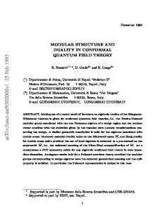
The diagram has a physical interpretation as crossing symmetry. Note that there is an additional way applying the associativity of the OPE in case of the 4-point function leading to another diagram and two further equalities. A conformal field theory can also be defined on arbitrary Riemann surfaces ins stead of C. Then the F r , F depend only on the complex structure of the surface. Finally, they can be considered as holomorphic sections on the appropriate

168


moduli spaces with values in suitable line bundles (cf. [FS87], [TUY89], [KNR94], [Uen95], [Sor95], [Bea95], [Tyu03*] and Chap. 11). In any case a conformal field theory has to satisfy – in addition to the Axioms 1–5 – the following axiom: Axiom 6 (Operator Product Expansion) The primary fields have the OPE (9.10). This OPE is associative. Concluding Remarks: 1. All n-point functions of the primary fields can be derived from the Gi for i ∈ B41 . 2. The expansions (9.10) are the fusion rules, which can be written formally as [Φi ] × [Φ j ] =

∑ [Φl ],

l∈B1

or, carrying more information, as Φi × Φ j = ∑ Nilj Φl , l

where Nilj ∈ N0 is the number of occurrences of elements of the family [Φl ] in the OPE of Φi (z)Φ j (0). The coefficients Nikj define the structure of a fusion ring, cf. Sect. 11.4. 3. We have sometimes passed over to radial quantization, e.g., by using Cauchy integrals in Sect. 9.2, for instance L−n (z) =

1 2π i

3

T (ζ ) dζ . (ζ − z)n+1

4. To construct interesting examples of conformal field theories satisfying Axioms 1–6 it is reasonable to begin with string theory. On a more algebraic level this amounts to study Kac–Moody algebras (cf. pp. 65 and 196). This subject is surveyed, e.g., in [Uen95] where an interesting connection with the presentation of conformal blocks as sections in certain holomorphic vector bundles is described (cf. also [TUY89] or [BF01*]). For other examples, see [FFK89].

9.4 Other Approaches to Axiomatization In order to lay down the foundations of conformal field theory introduced in [BPZ84], Moore and Seiberg proposed the following axioms for a conformal field theory in [MS89]:

References

169

A conformal field theory is a Virasoro module V=

W (ci , hi ) ⊗W (ci , hi )

i∈B1

with unitary highest-weight modules W (ci , hi ), W (ci , hi ) (cf. Sect. 6), subject to the following axioms: P 1. There is a uniquely determined vacuum vector Ω = |0 ∈ V with Ω ∈ W (ci0 , hi0 ) ⊗W (ci0 , hi0 ), hi0 = hi0 = 0. Ω is SL(2, C) × SL(2, C)-invariant. P 2. To each vector α ∈ V there corresponds a field Φα , i.e. an operator Φα (z) on V , z ∈ C. Moreover, there exists a conjugate Φα such that the OPE of Φα Φα contains a descendant of the unit operator. P 3. The highest-weight vectors α = i = vi of W (ci , hi ) determine primary fields Φi . Similarly for the highest-weight vectors of W (ci , hi ). P 4. Gi (z) = Ω|Φi1 (z1 ) . . . Φin (zn )|Ω , |z1 | > . . . > |zn |, always has an analytical continuation to Mn . P 5. The correlation functions and the one-loop partition functions are modular invariant (cf. [MS89]). Another axiomatic description of conformal field theory was proposed by Segal in [Seg91], [Seg88b], [Seg88a]. The basic object in this ansatz is the set of equivalence classes of Riemann surfaces with boundaries, which becomes a semi-group by defining the product of two such Riemann surfaces by a suitable fusion or sewing (cf. Sect. 6.5). Friedan and Shenker introduced in [FS87] a different, interesting system of axioms, which also uses the collection of all Riemann surfaces as a starting point. All these approaches can be formulated in the language of vertex algebras which seems to be the right theory to describe conformal field theory. In the next chapter we present a short introduction to vertex algebras and their relation to conformal field theory. Along these lines, the course of V. Kac [Kac98*] describes the structure of conformal field theories as well as the book of E. Frenkel and D. Ben-Zvi [BF01*]. A more general point of view is taken by Beilinson and Drinfeld in their work on chiral algebras [BD04*] where the theory of vertex algebras turns out to be a special case of a much wider theory of chiral algebras. A comprehensive account of different developments in conformal field theory is collected in the Princeton notes on strings and quantum field theory of Deligne and others [Del99*].

References [Bea95]

[BD04*]

A. Beauville. Vector bundles on curves and generalized theta functions: Recent results and open problems. In: Current Topics in Complex Algebraic Geometry. Math. Sci. Res. Inst. Publ. 28, 17–33, Cambridge University Press, Cambridge, 1995. A. Beilinson and V. Drinfeld. Chiral Algebras. AMS Colloquium Publications 51, AMS, Providence, RI, 2004.

170 [BPZ84]


A.A. Belavin, A.M. Polyakov, and A.B. Zamolodchikov. In- finite conformal symmetry in two-dimensional quantum field theory. Nucl. Phys. B 241 (1984), 333–380. [BF01*] D. Ben-Zvi and E. Frenkel. Vertex Algebras and Algebraic Curves. AMS, Providence, RI, 2001. [Del99*] P. Deligne et al. Quantum Fields and Strings: A Course for Mathematicians I, II. AMS, Providence, RI, 1999. [DMS96*] P. Di Francesco, P. Mathieu, and D. Sénéchal. Conformal Field Theory. SpringerVerlag, Berlin, 1996. [FFK89] G. Felder, J. Fröhlich, and J. Keller. On the structure of unitary conformal field theory, I. Existence of conformal blocks. Comm. Math. Phys. 124 (1989), 417–463. [FS87] D. Friedan and S. Shenker. The analytic geometry of two-dimensional conformal field theory. Nucl. Phys. B 281 (1987), 509–545. [Gaw89] K. Gawedski. Conformal field theory. Sém. Bourbaki 1988–89, Astérisque 177–178 (no 704) (1989) 95–126. [Gin89] P. Ginsparg. Introduction to Conformal Field Theory. Fields, Strings and Critical Phenomena, Les Houches 1988, Elsevier, Amsterdam, 1989. [HS66] N.S. Hawley and M. Schiffer. Half-order differentials on Riemann surfaces. Acta Math. 115 (1966), 175–236. [IZ80] C. Itzykson and J.-B. Zuber. Quantum Field Theory. McGraw-Hill, New York, 1980. [Kac98*] V. Kac. Vertex Algebras for Beginners. University Lecture Series 10, AMS, Providencs, RI, 2nd ed., 1998. [Kak91] M. Kaku. Strings, Conformal Fields and Topology. Springer Verlag, Berlin, 1991. [KNR94] S. Kumar, M. S. Narasimhan, and A. Ramanathan. Infinite Grassmannians and moduli spaces of G-bundles. Math. Ann. 300 (1994), 41–75. [LM76] M. Lüscher and G. Mack. The energy-momentum tensor of critical quantum field theory in 1 + 1 dimensions. Unpublished Manuscript, 1976. [MS89] G. Moore and N. Seiberg. Classical and conformal field theory. Comm. Math. Phys. 123 (1989), 177–254. [OS73] K. Osterwalder and R. Schrader. Axioms for Euclidean Green’s functions I. Comm. Math. Phys. 31 (1973), 83–112. [OS75] K. Osterwalder and R. Schrader. Axioms for Euclidean Green’s functions II. Comm. Math. Phys. 42 (1975), 281–305. [Seg88a] G. Segal. The definition of conformal field theory. Unpublished Manuscript, 1988. Reprinted in Topology, Geometry and Quantum Field Theory, U. Tillmann (Ed.), 432– 574, Cambridge University Press, Cambridge, 2004. [Seg88b] G. Segal. Two dimensional conformal field theories and modular functors. In: Proc. IXth Intern. Congress Math. Phys. Swansea, 22–37, 1988. [Seg91] G. Segal. Geometric aspects of quantum field theory. Proc. Intern. Congress Kyoto 1990, Math. Soc. Japan, 1387–1396, 1991. [Sor95] C. Sorger. La formule de Verlinde. Preprint, 1995. (to appear in Sem. Bourbaki, année 95 (1994), no 793) [TUY89] A. Tsuchiya, K. Ueno, and Y. Yamada. Conformal field theory on the universal family of stable curves with gauge symmetry. In: Conformal field theory and solvable lattice models. Adv. Stud. Pure Math. 16 (1989), 297–372. [Tyu03*] A. Tyurin. Quantization, Classical and Quantum Field Theory and Theta Functions, CRM Monograph Series 21 AMS, Providence, RI, 2003. [Uen95] K. Ueno. On conformal field theory. In: Vector Bundles in Algebraic Geometry, N.J. Hitchin et al. (Eds.), 283–345. Cambridge University Press, Cambridge, 1995.