Joint 48th IEEE Conference on Decision and Control and 28th Chinese Control Conference Shanghai, P.R. China, December 16-18, 2009
ThC06.6
Fractional Order Proportional and Derivative Controller Synthesis for A Class of Fractional Order Systems: Tuning Rule and Hardware-in-the-loop Experiment Ying Luo‡ , HongSheng Li† and YangQuan Chen§ Abstract— In recent years, fractional order systems have attracted more and more attention in various field, studies on real systems have revealed inherent fractional order dynamic behavior. It is intuitively true that these fractional order models require the corresponding fractional order controllers to achieve excellent performance. In this paper, a fractional order P D µ controller is designed systematically, to control a class of fractional order systems, the performance of the proposed P D µ controller designed for the fractional order system is compared with both the integer order and fractional order controllers which are designed for the approximate integer order system in the simulation and the hardware-in-the-loop experiment respectively. Index Terms— Fractional calculus; fractional order system, fractional order controller; P I λ D µ controller; iso-damping; gain variations; hardware-in-the-loop; dynamometer.
I. I NTRODUCTION Recently, fractional order systems have attracted more and more attention in various field, studies on real systems have revealed inherent fractional order dynamic behavior. Mechanical systems are described by fractional-order state equations [1][2][3]; in electricity, several applications have proposed a concept of fractance, which has intermediate properties between resistance and capacitance [4][5][6][7]; many real systems in bioengineering are modeled or fitted by fractional order systems [8][9]; new fractional derivative-based models have been demonstrated in [10][11][12][13], which provide powerful instrument for the description of memory and hereditary effects in various substances. Fractional order systems could model various real materials more adequately than integer order ones and thus provide an excellent modeling tool in describing many actual dynamical processes. It is intuitively true that these fractional order models require the corresponding fractional order controllers to achieve excellent performance. In most cases, however, researchers consider the fractional order controller applied to the integer order plant to enhance the system control performance [14][15]. The significance of fractional order control is that it is a generalization of classical integral order control theory, which could lead to more adequate and more robust control performance [15][16]. In general, there is no systematic way of designing proper fractional order controller (FOC) for the fractional order system (FOS). However, we may be able to get practical and simple FOC parameters tuning methods for certain specific fractional order plants. In this paper, a fractional order PD (FO-PD) controller is designed systematically for a class of fractional order systems, the performance of the proposed FO-PD controller designed for the fractional order system is compared with both the integer order and the fractional order controllers designed for the approximate integer order system (IOS) in the simulation and the hardware-in-the-loop (HIL) experiment respectively. The major contributions of this paper include 1)A fractional order P Dµ controller systematic design procedure for a class of fractional order systems, which can achieve favorable dynamic performance §
[email protected]; Dept. of Automation Science and Engineering, South China University of Technology, Guangzhou, P. R. China; Ying Luo was an Exchange Ph.D in Dept. of Electrical and Computer Engineering, Utah State University, Logan, UT, USA; †
[email protected]; with the Dept. of Automatic Engineering, Nanjing Institute of Technology, Jiangsu, P R China. ‡
[email protected]; Tel: 01(435)797-0148; Fax: 01(435)797-3054; Center for Self-Organizing and Intelligent Systems, Electrical and Computer Engineering department, Utah State University, Logan, UT 84341, USA. URL: http://www.csois.usu.edu/people/yqchen.
978-1-4244-3872-3/09/$25.00 ©2009 IEEE
and robustness; 2) Simulation performance comparison between the proposed FO-PD controller designed for the fractional order system and the integer/fractional order controllers which are designed for the approximate integer order system; 3) HIL experiment validation for the simulation results. The remaining part of this paper is organized as follows. In Sec. II, the fractional order system and the fractional order controller considered are introduced briefly and in Sec. III, a new tuning method for fractional order P Dµ controller design is proposed for the class of fractional order systems. The FO-PD controller can ensure that the given gain crossover frequency and phase margin are achieved and the phase derivative w. r. t. the frequency is zero, i.e., phase Bode plot is flat, at the gain crossover frequency. The simulation illustration and the HIL experiment validation are presented in Sec. IV and Sec. V, respectively. Finally, conclusions are given in Sec. VI. II. I NTRODUCTION FOR THE F RACTIONAL O RDER S YSTEM AND F RACTIONAL O RDER C ONTROLLER C ONSIDERED The fractional order system discussed in this paper is the fractional calculus model of Membrane Charging [9], which has the following form: 1 P (s) = . (1) s(T sα + 1) Note that, the plant gain is normalized to 1 without loss of generality since the proportional factor in the transfer function (1) can be incorporated in Kp of the system controller.
u(t)
I mo
Vm(t)
Switch closes at t =0
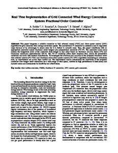
Fig. 1.
Rm
Cm D
Membrane charging circuit
The schematic diagram for the circuit of Membrane Charging is shown in Fig. 1, we can obtain the fractional order differential equation, α Vm (t) α d Vm (t) Cm = Imo u(t), (2) + dtα Rm applying the Laplace transformation to (2), and the Caputo representation for the fractional derivative [17] is chosen, then we can obtain, K Vm (s) = , (3) s(T sα + 1) α where K=Imo Rm , T =Rm Cm , with initial condition Vm (0+ )=0. Using the table of Inverse Laplace Transforms, we can find a solution in terms of the two parameters Mittag-Leffler function, which can be written as,
tα tα Eα,α+1 (− ). (4) T T This generalized fractional capacitor membrane model plays an important role in describing the dielectric behavior of membranes,
5460
Vm (t) = Imo Rm
ThC06.6 cells, tissues and variety of biological materials, for example, nerve, muscle, skin and so on [9]. The fractional order proportional and derivative controller considered in this paper has the following form of transfer function: C(s) = Kp (1 + Kd sµ ),
(5)
where µ∈(0, 2). Clearly, this is a specific form of the most common P I λ Dµ controller which involves an integrator of order λ (λ = 0, in this paper) and a differentiator of order µ. III. FO-PD C ONTROLLER D ESIGN P ROCEDURE FOR THE C LASS OF F RACTIONAL O RDER P LANTS In this paper, we restrict our attention to the class of fractional order plants P (s) described by (1). The transfer function of FO-PD considered has the form of (5).
(ii) Robustness to variation in the gain of the plant d(Arg(G(jω))) )ω=ωc = 0, dω with the condition that the phase derivative w. r. t. the frequency is zero, i.e., the phase Bode plot is flat, at the gain crossover frequency. It means that the system is more robust to gain changes and the overshoots of the responses are almost the same. (iii) Gain crossover frequency specification (
|G(jωc )|dB = |C(jωc )P (jωc )|dB = 0. C. Numerical Computation Process 1) For integer order PD controller (µ = 1 in (5)): From (13) and according to Specification (ii):
P (jw)
1 (jω)(T (jω)α + 1) 1 (jω)[T ω α (cos απ + j sin απ ) + 1] 2 2 1 −T ω 1+α sin απ + j(ω + T ω 1+α cos 2
= = =
Arg[P (jω)]
=
|P (jω)|
=
(T ω 1+α sin
απ 2 ) 2
=
we arrive at Kd = απ , ) 2
(6)
where N =
1±
+ (ω + T ω 1+α cos
απ 2 ) 2
(8)
α−1 ωc αT sin απ 2
, and
2α +2T ω α cos απ 1+T 2 ωc c 2
Fractional order P D controller described by (5) can be written as, =
Kp (1 + Kd (jω)µ )
=
Kp [(1 + Kd ω µ cos
(Arg[G(jω)])ω=ωc
Arg[C(jω)] = tan
sin
µπ µπ ) + jKd ω µ sin ], (9) 2 2
(1−µ)π + Kd ω µ 2 (1−µ)π cos 2
(1 − µ)π − , 2
(10)
µπ 2 µπ 2 ) + (Kd ω µ sin ) . (11) 2 2 The open-loop transfer function G(s) is that,
|C(jω)| = Kp
q
(1 + Kd ω µ cos
G(s) = C(s)P (s),
(12)
from (7) and (10), the phase of G(s) is as follows, Arg[G(jω)]
=
tan
−1
−π −
(1−µ)π + Kd ω µ 2 + cos (1−µ)π 2 T ω α sin απ 2 tan−1 1 + T ω α cos απ 2
sin
= =
Arg[C(jωc )P (jωc )] −π + φm ,
= =
µπ − π − tan 2 −π + φm φ,
sin απ 2 1 + T ω α cos απ 2 (14)
According to Specification (ii) about the robustness to gain variations in the plant: ( =
(13)
d(Arg(G(jω))) )ω=ωc dω µ−1 µKd ωc cos (1−µ)π 2
cos2
(1−µ)π 2
+ (sin
(1−µ)π 2
(α−1)
B. Design Specifications Here, three interesting specifications to be met by the fractional order P Dµ controller are proposed. From the basic definitions of gain crossover frequency and phase margin: (i) Phase margin specification Arg[G(jωc )]
(1−µ)π + Kd ωcµ 2 (1−µ)π cos 2 T ωα −1
tan−1
from (14), the relationship between Kd and µ can be established as follows: T ω α sin απ 1 µπ −1 2 Kd = tan[φ + tan − ] m ωcµ 1 + T ω α cos απ 2 2 (1 − µ)π (1 − µ)π 1 cos − µ sin . (15) 2 ωc 2
µπ 2 .
sin
=
+
the phase and gain are as follows, −1
1 + T ωcα cos απ 2 ). T ωcα sin απ 2
That means the Specifications (i) and (ii) can not be satisfied simultaneously for traditional PD controller. 2) For fractional order P Dµ controller : According to Specification (i), the phase of G(s) can be expressed as:
µ
C(jω)
= 0,
1 − 4N 2 ωc2 , 2N ωc2
(7) .
απ 2
√
Arg[G(jω)] = tan−1 (Kd ωc ) + tan−1 (
T ω α sin απ π 2 − − tan−1 , 2 1 + T ω α cos απ 2 1
p
d(Arg(G(jω))) )ω=ωc dω αT sin απ ωcα−1 Kd 2 − 2α 2 2 1 + (Kd ωc ) 1 + T ωc + 2T ωcα cos
(
A. Preliminary The phase and gain of the plant in frequency domain can be given from (1) by,
− =
(T ω α
αT ω sin απ )2 + (1 2
+ Kd ωcµ )2
sin απ 2 + T ωα
cos
0,
απ 2 ) 2
(16)
from (16), we can establish an equation about Kd in the following form: Aωc2µ Kd2 + BKd + A = 0, (17) that is Kd =
where φm is the phase margin.
5461
−B ±
p
B 2 − 4A2 ωc2µ , 2Aωc2µ
(18)
ThC06.6 where A
=
(T ωcα sin
(α−1) sin απ αT ωc 2 απ 2 α ) + (1 + T ω c 2
cos
απ 2 , ) 2
(1 − µ)π (1 − µ)π − µωcµ−1 cos . 2 2 According to Specification (iii), we can establish an equation about Kp : B
2Aωcµ sin
=
|G(jωc )| |C(jωc )||P (jωc )|
=
Kp
=
p
(1 + Kd ωcµ cos
p
(T ω 1+α sin
=
απ 2 ) 2
µπ 2 ) 2
+ (Kd ωcµ sin
+ (ω + T ω 1+α cos
µπ 2 ) 2 απ 2 ) 2
1.
(19)
Clearly, we can solve equations (15), (18) and (19) to get µ, Kd and Kp . D. Design Procedure Summary It can be observed from (15) and (18) that µ and Kd can be obtained jointly. But, it is complex to get the analytical solution of µ and Kd as the equations (15) and (18) are complicated. Fortunately, a graphical method can be used as a practical and simple way to get µ and Kd because of the plain forms about (15) and (18). The procedure to tune the fractional order P Dµ controller are as follows: (1) Given ωc , the gain crossover frequency; (2) Given Φm , the desired phase margin; (3) Plot the curve 1, Kd w. r. t µ, according to (15); (4) Plot the curve 2, Kd w. r. t µ, according to (18); (5) Obtain the µ and Kd from the intersection point on the above two curves; (6) Calculate the Kp from (19). Remark 3.1: Design specifications should not be chosen too aggressive because of the constraint in (18) and the intersection point needed on the two curves above.
100 50 Magnitude (dB)
Gf (s) = K
N Y s + ωk′
k=−N
s + ωk
,
(20)
where the zeros, poles and the gain can be evaluated from 1
ωk′ = ωb (
+ (1−γ) 2 ωh k+N2N +1 , ) ωb
ωk = ωb (
+ (1+γ) 2 ωh k+N2N +1 , ) ωb
(21)
1
K=(
(22)
N ωh − γ2 Y ωk ) . ωb ωk′
(23)
k=−N
In our simulation, for approximation of fractional order differentiator sµ , the frequency range of practical interest is set to be from 0.0001Hz to 10000Hz. For the comparison purpose, the considered fractional order real system can be approximated by a typical second order system as shown in (24), K P (s)app = , (24) s(T s + 1) which can model a DC motor position servo system. In order to compare the controllers designed for approximate integer order system (IOS) with the ones designed for the real fractional order system (FOS) fairly, three simulation cases are presented. • Case-1: The optimal P controller and the FO-PD controller designed for the approximate IOS simulation test for the approximate IOS; • Case-2: The optimal P controller and the FO-PD controller designed for the approximate IOS simulation test for the real FOS; • Case-3: The FO-PD controller designed for the real FOS simulation test for the FOS;
Bode Diagram
0 −50 −100 −150 −70 −80
Phase (deg)
(19) easily, that is Kp = 10.916. The Bode diagrams of the openloop system designed are shown in Fig. 2. As can be seen, the gain crossover frequency specification, ωc = 10(rad/sec), and phase margin specification, Φm = 70o , are fulfilled. The phase is forced to be flat at ωc . Actually, the fractional order system and the fractional order P Dµ controller are infinite dimensional due to the fractional order differentiator α and µ. A band-limit implementation is important in practice. Finite dimensional approximation of the FOS and FOC should be utilized in a proper range of frequency of practical interest. The approximation method in this paper is the Oustaloup Recursive Algorithm [18]. Assuming the frequency range to fit is selected as (ωb , ωh ). The approximate transfer function of a continuous filter for sγ with Oustaloup Algorithm is as follows:
−90 −100
8 Kp=1.000 Kp=1.125 Kp=1.250 Kp=1.375 Kp=1.500
−110 −2
10
−1
10
0
10
1 2 3 10Frequency10(rad/sec) 10
4
10
5
10
7
6
10
6
Bode diagram with fractional order P D µ controller
5
IV. S IMULATION I LLUSTRATION For the real fractional order system, the P Dµ fractional order controller design method above is illustrated via a numerical simulation. In the simulation, the plant parameter T and α in (1) are chosen as 0.4s and 1.4 respectively. The specifications of interest are set as ωc =10(rad./sec.), Φm =70o , and the robustness to gain variations in the plant is required. From (15) and (18), two curves can be plotted easily. One can obtain the µ and Kd obviously from the intersection point on the two curves, that is µ = 1.189 and Kd = 0.6138. Then Kp can be calculated from
Position (rads)
Fig. 2.
4
3
2
1
0
0
1
2
3
4
5 Time (seconds)
6
7
8
9
10
Fig. 3. Simulation. Step responses with the ITAE optimum P controller designed for the approximate IOS for the IOS
5462
ThC06.6 8
8 Kp=11.088 Kp=12.474 Kp=13.860 Kp=15.246 Kp=16.632
7
6
6
5 Position (rads)
Position (rads)
5
4
3
3
2
1
1
0
1
2
3
4
5 Time (seconds)
6
7
8
9
0
10
Fig. 4. Simulation. Step responses with the FO-PD controller designed for the approximate IOS for the IOS
1
2
3
4
5 Time (seconds)
6
7
8
9
10
8 Kp=1.000 Kp=1.125 Kp=1.250 Kp=1.375 Kp=1.500
7
6
6
Position (seconds)
4
3
5
4
3
2
2
1
1
0
1
2
3
4
5 Tiime (seconds)
6
7
8
9
Kp=8.733 Kp=9.825 Kp=10.916 Kp=12.008 Kp=13.099
7
5
0
0
Fig. 6. Simulation. Step responses with the FO-PD controller designed for the approximate IOS for the real FOS
8
Position (rads)
4
2
0
Kp=11.088 Kp=12.474 Kp=13.860 Kp=15.246 Kp=16.632
7
0
10
0
1
2
3
4
5 Time (seconds)
6
7
8
9
10
Fig. 5. Simulation. Step responses with the ITAE optimum P controller designed for the approximate IOS for the real FOS
Fig. 7. Simulation. Step responses with the FO-PD controller designed for the real FOS for the FOS
A. Case-1: The optimal P controller and the FO-PD controller designed for the approximate IOS simulation test for the IOS
can see both of the results are not satisfied, which confirms that this fractional order system model may require the corresponding fractional order controller to achieve expectative performance.
In this case, the traditional P controller and the FO-PD controller are designed and tested for the approximate integer order model (24). It is well-known that proportional controller is adopted commonly for the typical second order plant (24), and the ITAE optimum proportional parameter is K=1/2T [19], therefore, proportional parameter is set as 1.25 in this example. The FO-PD controller can also be designed for this integer order approximation following our proposed procedures, this integer order system is just a special case of the fractional order system considered. The specifications of interest are also set as ωc = 10(rad./sec.), Φm = 70o , and the robustness to gain variations in the plant is required. Following our design procedure, one can obtain that µ = 0.844, Kd = 0.368 and Kp = 13.860. In Fig. 3, applying the ITAE optimal proportional controller, the unit step responses are plotted with the open-loop plant gain varying from 1 to 1.5 (±20% variations from the desired value 1.25). In Fig. 4, applying fractional order P Dµ controller, the unit step responses are plotted with open-loop gain changing from 11.088 to 16.632 (±20% variations from the desired value 13.86). It can be seen from Fig. 3 and Fig. 4 that the fractional order P Dµ controller designed by the proposed method is effective, and performances better than the optimum P controller for the approximate IOS. B. Case-2: The optimal P controller and the FO-PD controller designed for the approximate IOS simulation test for the real FOS If the optimum P controller and the FO-PD controller, which are designed in Case-1 for the approximate IOS, are used to control the real FOS, from Figs. 5 and 6, which also plotted the five unit step responses for the ITAE optimal P controller and the FO-PD controller with the open-loop plant gain varying from the lower ±20% to the upper ±20% of the desired value respectively, we
C. Case-3: The FO-PD controller designed for the real FOS simulation test for the FOS In this case, as mentioned before, when the specifications are set as ωc = 10(rad./sec.), Φm = 70o , and the robustness to gain variations in the plant is required, according to the real FOS and following the proposed design procedures, the FO-PD controller parameters are designed as µ = 1.189, Kd = 0.6138 and Kp = 10.916. Figure. 7 shows the effectiveness of the systematic designed FOPD controller tested for the real FOS, the unit step responses are also plotted with open-loop gain changing from 8.733 to 14.099 (±20% variations from the desired value 10.916). Comparing with Fig. 5 and Fig. 6, the overshoots of the position step responses are much smaller and there is no oscillation. Especially, the five responses almost follow the same curve, the robustness to the gain variation of the system is excellent. V. E XPERIMENT VALIDATION In this section, the practicality of the proposed FO-PD controller design scheme and the performance advantages of the FO-PD controller for the FOS presented in the simulation are also validated in a hardware-in-the-loop (HIL) experimental test bench. A. HIL Experimental Setup A fractional horsepower dynamometer was developed as a general purpose experiment platform [20]. The architecture of the dynamometer control system is shown in Fig. 8. The dynamometer includes the DC motor to be tested, a hysteresis brake for applying torque load to the motor, a load cell to provide force feedback, an optical encoder for position feedback and a tachometer for velocity feedback. The dynamometer was modified to connect to a Quanser
5463
ThC06.6 8 Kp=1.000 Kp=1.125 Kp=1.250 Kp=1.375 Kp=1.500
7
6
Position (rads)
5
4
3
2
1
The dynamometer setup
0
MultiQ4 terminal board in order to control the system through Matlab/Simulink Real-Time Workshop (RTW) based software. This terminal board connects with the Quanser MultiQ4 data acquisition card. Then, use the Matlab/Simulink environment, which uses the WinCon application from Quanser, to communicate with the data acquisition card. This enables rapid prototyping and experiment capabilities to many linear/nonlinear models of arbitrary form. Without loss of generality, consider the servo control system modeled by:
0
1
2
3
4
5 Time (seconds)
6
7
8
9
10
Fig. 10. Experiment. Step responses with the ITAE optimum P controller designed for the original dynamometer IOS for the IOS 8 Kp=11.088 Kp=12.474 Kp=13.860 Kp=15.246 data5
7
6
5 Position (rads)
Fig. 8.
4
3
x(t) ˙ = v(t), v(t) ˙ = Ku u(t) − Kb v.
(25) (26)
2
1
where x is the position state, v is the velocity, and u is the control input, Ku and Kb are positive coefficients. B. HIL Emulation of the FOS Through simple system identification process, the dynamometer position control system can be approximately modeled by a transfer 1.52 function s(0.4s+1) , which can be treated as the approximate integer order system (24). The fractional order system (1) can be emulated by modifying the dynamometer hardware-in-the-loop test bench as shown in Fig. 9, P (s) = Gm (s)(
KA(s) KB(s) 1 1 + ) , 1 + KA(s) 1 + KB(s) 1s K s
(27)
where Gm (s) =
1 1 , A(s) = s−α , B(s) = s−α+1 , K = , Ts + 1 T
and Gm (s) s1 is the model of the dynamometer position control system with T = 0.4s and modifying the DC gain of the model as 1 without loss of the generality. So, we can calculate the designed fractional order system from (27) as follows, 1 . (28) P (s) = s(T sα + 1) The modules A(s) and B(s) in Fig. 9 are also implemented using the fractional order operator module sγ with Oustaloup Algorithm introduced in Sec. IV.
0
0
1
2
3
4
5 Time (seconds)
6
7
8
9
10
Fig. 11. Experiment. Step responses with the FO-PD controller designed for the original dynamometer IOS for the IOS
C. Experimental Results Substituting the original dynamometer bench and the modified dynamometer platform for the approximate integer order model and the fractional order system in the simulation respectively, the optimum P controllers and designed FO-PD controllers in the three simulation cases are all tested in this hardware-in-the-loop manner. First, designed for the original dynamometer IOS, and tested for the original dynamometer setup, Fig. 10 and Fig. 11 show the unit step position responses using the ITAE optimal P controller and the FO-PD controller. Second, designed also for the original dynamometer IOS, but tested for the modified dynamometer FOS, Fig. 12 and Fig. 13 present the unit step position responses using the ITAE optimal P controller and the FO-PD controller respectively. Third, designed for and also tested for the modified dynamometer FOS, Fig. 14 shows the unit step position responses using the FOPD controller designed by the proposed tuning method in this paper. Comparing with Figs. 12 and 13, it is obvious that, in Fig. 14 with the properly designed FO-PD controller, the overshoots of the position step responses are much smaller and there is no oscillation; especially, the five responses almost follow the same curve, the robustness to the gain variation of the system is excellent. So, the simulation results are validated in our HIL experimental platform. VI. C ONCLUSIONS
Fig. 9.
The fractional order system by modifying the dynamometer
In this paper, we have proposed a tuning method for fractional order proportional and derivative controller for a class of fractional order plants. According to the fractional order system considered, the FO-PD controller is tuned to ensure that the given gain crossover frequency and the phase margin are achieved and the phase derivative w. r. t. the gain crossover frequency is zero, i.e., the phase Bode plot is flat, at the gain crossover frequency, so that the closedloop system is robust to gain variations and the step responses exhibit iso-damping property. The FO-PD controller tuning method proposed in the paper, aiming at a class of fractional order plants,
5464
ThC06.6 8
8 Kp=1.000 Kp=1.125 Kp=1.250 Kp=1.375 Kp=1.500
7
6
6
5 Position (rads)
Position (rads)
5
4
4
3
3
2
2
1
1
0
Kp=8.733 Kp=9.825 Kp=10.916 Kp=12.008 Kp=13.099
7
0
1
2
3
4
5 Time (seconds)
6
7
8
9
0
10
Fig. 12. Experiment. Step responses with the FO-PD controller designed for the original dynamometer IOS for the modified dynamometer FOS
0
1
2
3
4
5 Time (seconds)
6
7
8
9
10
Fig. 14. Experiment. Step responses with the FO-PD controller designed for the modified dynamometer FOS for the FOS
8 Kp=11.088 Kp=12.474 Kp=13.860 Kp=15.246 Kp=16.632
7
6
Position (rads)
5
4
3
2
1
0
0
1
2
3
4
5 Time (seconds)
6
7
8
9
10
Fig. 13. Experiment. Step responses with the FO-PD controller designed for the original dynamometer IOS for the modified dynamometer FOS
is practical, simple and systematic. Simulation and experimental results show that the closed-loop system can achieve favorable dynamic performance and robustness with the properly designed FO-PD controller for the fractional order system considered.
[13] M. Caputo and F. Mainardi, “A new dissipation model based on memory mechanism,” Pure and Appl. Geophysics, vol. 91, no. 8, pp. 134–147, 1971. [14] D. Y. Xue, C. N. Zhao, and Y. Q. Chen, “Fractional order PID control of a DC motor with elatic shaft: A case study,” in Proc. of American Control Conference (ACC), Minnesota, USA, 2006, pp. 3182–3187. [15] HongSheng Li, Ying Luo, and YangQuan Chen, “Fractional order proportional and derivative (FOPD) motion controller: Tuning rule and experiments,” IEEE Trans. on Control System Technology (in press). [16] I. Podlubny L. Dorcak and I. Kostial, “On fractional derivatives, fractional-order dynamic system and PID-controllers,” in IEEE Proc. of the 36th CDC, San Diego, California USA, December 1997. [17] I. Podlubny, “Fractional Differential Equations,” Academic Press, 1999. [18] A. Oustaloup, J. Sabatier, and P. Lanusse, “From fractional robustness to CRONE control,” Fractional Calculus and Applied Analysis, vol. 2, no. 1, pp. 1–30, 1999. [19] Richard C. Dorf and Robert H. Bishop, “Modern control systems,” Pearson Prentice Hall, Pearson Education, Upper Saddle River, pp. 270–278, 2005. [20] Y. Tarte, YangQuan Chen, Wei Ren, and K. Moore, “Fractional horsepower dynamometer - a general purpose hardware-in-the-loop realtime simulation platform for nonlinear control research and education,” in IEEE Conference on Decision and Control, 13-15 Dec. 2006, pp. 3912 – 3917.
R EFERENCES [1] R. L. Bagley and R. A. Calico, “Fractional-order state equations for the control of viscoelastic damped structures,” J. Guidance, Control and Dynamics, vol. 14, no. 2, pp. 304–311, 1991. [2] R. L. Bagley and P. Torvik, “On the appearance of the fractional derivative in the behavior of real materials,” J. Appl. Mech., vol. 51, pp. 294–298, 1984. [3] A. Makroglou, R. K. Miller, and S. Skaar, “Computational results for a feedback control for a rotating viscoelastic beam,” J. Guidance, Control and Dynamics, vol. 17, no. 1, pp. 84–90, 1994. [4] A. Le Mehaute and G. Crepy, “Introduction to transfer and motion in fractal media: The geometry of kynetics,” Solid State Ionics, , no. 9-10, pp. 17–30, 1983. [5] M. Nakagawa and K. Sorimachi, “Basic characteristics of a fractance device,” IEICE Trans. Fundamentals, vol. E75-A, no. 12, pp. 1814– 1819, 1992. [6] K. B. Oldham and C. G. Zoski, “Analogue instrumentation for processing polarographic data,” J. Electroanal. Chem., vol. 157, pp. 27–51, 1983. [7] S. Westerlund, “Capacitor theory,” IEEE Trans. Dielectrics Electron. Insulation, vol. 1, no. 5, pp. 826–839, 1994. [8] YangQuan Chen, Dingyu Xue, and Huifang Dou, “Fractional calculus and biomimetic control,” in IEEE Int. Conf. on Robotics and Biomimetics (RoBio04), Shengyang, China, August 22-25 2004, pp. (PDF–robio2004–347). [9] Richard L. Magin, “Fractional calculus in bioengineering,” Begell house publishers Inc., 2006. [10] M. Caputo, “Elasticita e dissipacione,” Bologna: Zanichelli, 1969. [11] T. F. Nonnenmacher and W. G. Glockle, “A fractional model for mechanical stress relaxation,” Philosophical Magazine Lett., vol. 64, no. 2, pp. 89–93, 1991. [12] Ch. Friedrich, “Relaxation and retardation functions of the maxwell model with fractional derivatives,” Rheol. Acta., vol. 30, pp. 151–158, 1991.
5465


![Fractional-Order [Proportional Derivative] Controller for Robust Motion ...](https://m.moam.info/img/260x300/fractional-order-proportional-derivative-controlle_5bb87d99097c47550a8b4594.jpg)