FREIGHT MODAL ENERGY EFFICIENCY: A COMPARISON MODEL A. Parajuli, L. Ferreira and J. Bunker School of Civil Engineering, Queensland University of Technology Brisbane, Queensland
[email protected],
[email protected] Abstract This paper describes the findings of a state-of-the-art literature review on the energy consumption of land based freight transport modes and outlines the development of a model to compare corridor energy consumption of road and rail options. The key parameters influencing the energy estimation and comparison procedure are identified and a methodology to compare door to door freight movement is provided.
Apelbaum (1998) has also recorded the rising trend of energy efficiency on road until 1995.
Introduction
The Australian freight task is expanding rapidly. Doubling of the road freight task in the next twenty years has been estimated. The growth continues to be stronger than GDP (BTRE 2002). The relative share of freight between road, rail and sea has seen a significant change over the past twenty years. For the non-bulk freight task there has been considerable competition between the modes as can be seen in Figure 1.1.
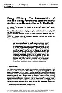
Figure 1.2 Australian energy efficiency
Energy efficiency (net ton km per MJ)
1.0
5.4 5.2 5 4.8 4.6 4.4 4.2 4 3.8 3.6 3.4 3.2 3 2.8 2.6 2.4 2.2 2 1.8 1.6 1.4 1.2 1 0.8 0.6 0.4 0.2 0
Australian
non-bulk
freight
Road Rail Sea
1975
Figure 1.1 movements
domestic
1984
1987
1990
1994
1997
Year
freight
Source: Laird (2003)
Freight Task (in B ln NtKm)
50 45
Total
40
Road
These issues raise concerns regarding freight mode choice based on energy consumption and the corresponding energy saving. The factors affecting the energy consumption are discussed.
Rail
35
Coastal shipping
30 25 20 15
2.0
10
Review of energy estimation models
5
95 19
91
93 19
19
87
89 19
19
83
85 19
19
79
77
81 19
19
19
75
73 19
19
19
71
0
Year
Source: BTE (1999) Laird (2003) reported the corresponding rise in the energy consumption in freight sector from 233.3 PJ in 1976 to 401.1 PJ in 1998 or a 72% increase. Laird (2003) summarized the efficiency of road, rail and sea. Figure 1.2 shows that energy efficiency of sea and rail improved substantially, particularly between 1984 and 1997. The increase in road energy efficiency is less distinct due to its inefficiency relative to the other two modes.
Energy estimation is based on the forces that the vehicle has to overcome in operation, including: • Rolling resistance; • Grade resistance; • Inertial resistance; and • Air resistance. Some additional energy is required to overcome driveline losses and to power vehicle accessories. Greenwood and Bennett (2001) presented a typical energy flow model of a passenger car. The same principles apply to freight vehicles. Figure 2.1
Model of energy flow
1
Idling
17.2%
Energy in fuel
2.2%
Engine
100%
2.6%
Accessories
Aerodynamic
18.2 %
Drive line
12.6
4.2%
Rolling 62.4%
5.6%
Engine loss (Waste heat)
Drive line losses
5.8%
Braking
Source: Greenwood and Bennett (2001) 2.1
Additional fuel consumption model types include: • Emission and carbon balance approach (Kent and Mudford 1979 and EC 1999) • Mechanistic approach (Wang et al 1992, Shayler et al 1999 and Meibom 2001)
Road transport models
Modelling the fuel consumption based on vehicle speed has been a common practice over the years (see Chang et al (1976), Bowyer et al (1985), Biggs (1988)). Ferreira (1985) developed an empirical relationship which also incorporated stop/start and slowing down. To better describe the fuel consumption in regression models, the terms such as rise, fall and roughness were introduced. Greenwood and Bennett (2001) reported the form of those equations as: Fuel consumptio n = A0 + ( A1 / v ) + ( A2 × v 2 ) + A3 × Rise + A4 × Fall + A5 × Roughness K K (1)
where: A0, A1, A2, A3, A4 and A5 are regression coefficients. Based on Bowyer et al (1985) and Biggs (1988), the energy consumption models could be classified into four groups, namely: • Average speed model; • Running speed model; • Four mode elemental model; and • Instantaneous model. Average speed models have been improved to include the effect of acceleration by West et al (1997) and Ahn et al (2002). Running speed models incorporate the average effect of grade and difference in running and idle phases. Bowyer et al (1985) reported that running speed models could underestimate fuel consumption over a trip and the error was related to the grade term. Four mode elemental models estimate fuel consumption more precisely by dividing the operating phases of vehicle into four different phases, namely: idle, cruise, acceleration and deceleration. Instantaneous models estimate fuel consumption in small time increments, thus increasing the accuracy.
Some of these low level models offer good predictive ability but suffer from complex data requirements that are not always available to be implemented on a corridor level. Post et al (1984) reported that the more aggregate models such as average and running speed models cannot estimate energy consumption well for short sections (less than 4 km) but their performance did not differ large for long trip (9km). This was accredited to the effect of negative power demand, for example due to downhill with some engine breaking, which may account for substantial proportion for short trip. BT (1995) reported age and type of vehicles in operation, condition of the equipment and standards for maintenance and repair, technologies used, terrain travelled and driver’s skill as major factors influencing fuel consumption. The NIMPAC style models use the following relationship to estimate the fuel consumption as a part of estimating vehicle operating cost (VOC) (Thoresen and Roper 1996). Fuel Consumptio n (litres/10 00km)
=
Engine Basic Fuel/Speed × 1 + Efficiency Adjustment Relationsh ip
Road Traffic Curvature Gradient + + + Roughness + Congestion Adjustment Adjustment Adjustment Adjustment
KKKKKKKKKKKK (2)
NIMPAC is easy to use and understand due to the simplicity of its algorithm. The input data set includes parameters that are easily available in the public domain. The model is used widely in Australia. The Queensland Department of Main Roads currently uses NIMPAC models for estimating VOC parameters for road project evaluation. It was found from a review of NIMPAC style models that one of the important missing parameters on fuel consumption subroutine is payload. This research focuses on freight movement comparison where
2
payload is of prime importance. The effect of payload has been investigated later. 2.2
Rail transport models
Kraay et al (1991) developed an energy consumption model for trains based on energy needed to overcome resistance along with an energy parameter related to change in kinetic energy. The resistance term accounts for grade, radius of curvature, gravity, air friction, rail friction and speed. A number of coefficients were adopted for correlating those terms with energy consumption, depending on train and track types. The energy consumption of a train has also been estimated using speed as a prime influencing factor. EC (1999) suggested two models for rail energy estimation, the first one as a function of average speed and distance between stops and the second based on steady state loading of the train, acceleration energy, deceleration energy and gradient energy. The generalised relationships are given below: 2 / ln( x) + C Energy consumption = k × Vavg KKKKKK(3) 2 / 2) Energy consumption = (( N stop + 1) / L) × (Vmax + B0 + B1 × Vavg 2 + g × ∆h / L + B2 × Vavg KKKKKK(4)
where: k and C are train dependent constants; x is distance between stops in km; Vavg and Vmax are average and maximum speed; Nstop is number of stops; ∆h is the difference in elevation; L is total trip length; and B0, B1 and B2 are empirical coefficients for the steady state load.
Several Australian Railway Association (ARA) rail fact sheets argue that rail freight transport consumes much less energy than road transport. However, this type of comparison, which is based only on line haul movement, does not provide the overall efficiency of the task. Modal energy comparisons should reflect the door to door task. The characteristics that need to be compared to fully understand energy consumption across the entire freight task are highlighted in figure 3.1. Figure 3.1
Comparison routes Origin
Collection
Road leg (pick up) Could be LCV or rigid truck or articulated truck
Total haulage by Road (by rigid or articulated truck)
Rail line haul
Collection
Road leg (pick up) Could be LCV or rigid truck
Road leg (delivery)
Could be LCV or rigid truck or articulated truck
Road line haul (by rigid or articulated truck)
Road leg (delivery)
Destination
Collection
Collection Could be LCV or rigid truck
Recent attempts to compare freight modal energy demand, such as ATC (1991), IFEU and SGKV (2002) and Affleck (2002), lack an analytical energy accounting framework necessary to thoroughly understand and describe the complete freight task’s energy consumption on many (and/or rest) of the Australian corridor. Houghton and McRobert (1998) started the work of model framework development for an energy based comparison between several options available for Australian land freight movement. This study focuses on developing a similar type of model with the inclusion of more explanatory variables that will quantify the traffic and terrain characteristics in terms of fuel use.
Here the models are reviewed for their suitability in corridor level analysis and comparison. IFEU and SGKV (2002) suggested some additional parameters influencing road and rail energy comparison study, such as weight restriction, shunting, intermodal transfers etc. Hence a prudent judgement prior to the evaluation of modal performance by an analytical model is desired.
4.0 Development of a Freight Energy Consumption Comparison Model
3.0
The discussion below describes aspects of development of the model.
Modal comparison of energy efficiency
In this research a model will be developed to compare the energy consumption on a net tonnekm (NTK) basis between the major land based freight modes, road and rail. A spreadsheet modelling tool is being developed.
3
4.1
more data, computer based vehicle simulation model and test runs.
Road transport
For the road section of the freight task, it is proposed to adopt the NIMPAC model with an additional correction factor related to payload term. The proposed model is: Fuel Consumptio n (litres/10 00km)
+
=
Payload Engine Basic Fuel/Speed × Correction × 1 + Efficiency Factor Adjustment Relationsh ip
Road Traffic Gradient Curvature + + Roughness + Congestion Adjustment Adjustment Adjustment Adjustment KKK KKKK (5)
Basic fuel/speed relationship The basic fuel/speed in the NIMPAC model relationship only purports how fuel consumption varies with vehicle speed, assuming steady speed operation over flat straight road. The basic fuel speed relationship is given as: Basic fuel / speed relationship = A + B / Speed + C × Speed 2 KKKKKKK(6)
Harmonised values for terms A, B and C for each of the vehicle types as reported by Thoresen and Roper (1996) and Thoresen (2003) are being considered for the estimation. Payload correction factor Payload has a significant impact on energy consumption. Ghojel and Watson (1995) reported a good linear fit between basic fuel consumption and payload. IFEU and SGKV (2002) also successfully used a multiplying factor to incorporate the effect of variation in payloads. It is already a tested approach to quantify a variation in payload as a multiplying factor. Load factor is to be used for quantifying the adjustment of fuel consumption. CSIRO, PPK and USA (2002) reported a linear fit of load factor and fuel consumption load correction factor. Payload correction term correlating the relationship between vehicle type and fuel consumption is yet to be fixed. Fuel consumption data (to be collected from freight operator/s) will be used to finalise the correction factor. Later it will be validated with
Adjustment factors The first adjustment factor in the NIMPAC model is the engine efficiency adjustment factor, which was modelled on state of tune factor (Thoresen 2003, pg 24). Thoresen (1988) reported that on an average the untuned vehicles consumed only about one per cent more fuel compared with their fuel use when tuned. The second adjustment factor in the equation is gradient adjustment. The gradient adjustment was quantified based on road gradient, vehicle type and corresponding speed. Curvature adjustment is the third adjustment factor which was modelled on degree of road curvature and vehicle type. For road roughness two separate factors were calculated (Pavement condition cost factor, GCFGAC and NIMPAC model variable, FCGRVF). GCGFAC adjusts for the effects of changing road roughness measured in NRM (counts per kilometre) and FCGRVF allows this impact to be varied by vehicle type and travel speed (Thoresen 2003). These factors are combined together for road roughness factor. The last adjustment factor is traffic congestion which was quantified based on Volume to Capacity Ratio (VCR) and NIMPAC model parameter namely FCONG. Traffic congestion adjustment is the product of VCR and FCONG where FCONG is the maximum value applicable regardless of whether VCR is higher than unity. 4.2
Rail transport
The review of various rail energy consumption model supports the inclusion of parameters related to speed, travel distance/number of stops, grade, curvature, length of the train and mass. Travel dis tan ce Grade Speed + A× = and / or term + B × and term Consumption term number of stops curvature Energy
Lengthof thetrain + C × and / or term Mass KKKKK (7)
4
A regression analysis is planned with the collection of data from rail operator/s. Sensitivity testing is also planned for determining the significance of those parameters. Speed term The forces opposing the motion of train are similar to those of a road vehicle. Hence it has been believed that the energy consumption could be modelled based on speed. Lukaszewicz (2001) and EC (1999) modelled the basic force required to propel train based on speed of the motion. FR = K0 + ( K1 × v) + ( K 2 × v2 ) KKK (8) Lukaszewicz (2001) has established a relationship between K0, K1 and K2 and train’s characteristics such as roller bearing resistance, mechanical resistance (such as deflection in the track, the wheel rail contact area, frictional forces in the wheel rail interference), length of the train, front and rear area etc. Adjustment factors Similar to road energy consumption modelling, the basic speed term only takes into account the energy demand of overcoming basic resistive forces over a flat straight section assuming the movement at approximately constant speed. EC (1999) successfully modelled the energy consumption of a train by combining the power required for resistance forces; similar to the one mentioned in Equation 8, with acceleration energy, and grade resistance energy in order to estimate the energy for more detailed route description. But the model lacks an ability to describe the effect of length and mass of the train independently. These are the desired flexibility in modal freight energy comparison model since the options may involve a large set of combinations ultimately affecting the freight energy efficiency measured in MJ per net tonne-km. This study is also approaching the modelling in the similar way, by first modelling the resistive forces with respect to velocity and then combining the effect of stop/start, grade, curvature, length and mass on the resistance overcoming forces with added understanding of the factors and collection of historical and current data. 4.3
Spreadsheet modelling tool
The spreadsheet has nine sheets namely: input freight characteristics, input road, input rail, vehicle characteristics, lookup tables, calculation, output road, output rail and summary table. The interrelationships between the sheets is summarised in Figure 4.1. The Input Freight Characteristics sheet allows the user to define, and later identify, the freight characteristics such as type of freight, size of freight and type of commodity. In some cases quantifying the energy used in terms of MJ per tonne-km would not totally describe other various aspects of freight task (BT 1995). The major deficiency of the measurement is the inability to deal with the volume of the task, which would govern the number of containers and trips ultimately affecting the final energy consumption. These parameters may be tallied at first so the user is better informed about the number of containers required to carry the commodity and trips generated for the task. The main aim of this sheet is to make an allowance for such judgement by informing users about the available volume and freight volume. The Input Road sheet allows user to input the freight movement characteristics of the pickup, road line haul and delivery section. Each pickup and delivery sections has been divided into three segments; each segment containing five rows (such as PU01 to PU05 for pickup leg). Each of those rows allows segregation based on traffic and terrain characteristics of freight task. If the pickup and delivery legs are more than one in number then each segment (that is five rows, distinguished by a colour) should be used for a single leg and later they could be identified with unique number (such as PU01 and PU05, De01 and De05) and accompanying start and end point’s detail. Road line haul section has three segments with fifteen rows in each segment. Each of those rows allows segregation based on traffic and terrain characteristics of freight. Three segments separated here allow three different vehicles of the same freight fleet to be considered at once for energy consumption comparison. Repeated run of the spreadsheet tool is necessary to encompass the energy performance of more number of vehicles on the fleet (more than three, if any) at once. Lookup table and calculation sheets quantify the adjustment factors.
5
Similarly the input rail sheet provides the user to input the freight movement characteristics involving road for pickup and delivery, and rail for line haul movement. Figure 4.1
The summary table sheet compares the energy required for pickup, line haul and delivery legs for options mentioned on input road sheet and input rail sheet to depict the overall modal freight energy.
Flow diagram of the comparison model Helps in identifying the freight task Informs users about the size of containers and number of trips required
Input Sheet
Freight characteristics Input road
Lookup tables
Estimating energy required for road movement section including pick up and delivery
Estimating energy required for rail movement section including road pick up and delivery
Input rail Output sheet
Road
Rail
Summary sheet (Comparison) 5.0
Conclusions and future work
There has been a significant growth in the Australian freight task accompanied by a corresponding increase in energy consumption. There is a large number of energy consumption models, some widely used and tested. A spreadsheet tool is under construction using the models reviewed with some adjustments. The spreadsheet tool compares the whole freight task from origin to destination, which will enable a thorough and unbiased comparison. The models to be used in the comparison tool are to be calibrated using data collected from freight operators and validated using a computer based vehicle simulation model. The spreadsheet tool will
be tested using a number of Queensland corridors. It will then be applied to compare the modal energy efficiency for specific movements. References Affleck. (2002). "Comparison of Greenhouse Gas Emission by Australian Intermodal Rail and Road Transport." Affleck Consulting, Brisbane. Ahn, K., Rakha, H., Trani, A. A., and Van Aerde, M. (2002). "Estimating Vehicle Fuel Consumption and Emissions based in Instantaneous Speed and Acceleration Levels." Journal of Transportation Engineering. Apelbaum. (1998). "The Queensland Transport Task: Primary Energy Consumed and Greenhouse Gas Emissions." Apelbaum Consulting Group Pty Ltd. ATC. (1991). "Rail vs Truck Fuel Efficiency: The relative fuel efficiency of truck competitive rail freight and truck
6
operations compared in a range of corridors." Abacus Technology Corporation, Chevy Chase. Biggs, D. C. (1988). "ARFCOM-Models for estimating light to heavy vehicle fuel consumption." ARR No. 152, Australian Road Research Board, Victoria. Bowyer, D. P., Akcelik, R., and Biggs, D. C. (1985). "Guide to fuel consumption analyses for Urban Traffic Management." Report Number 32, Australian Road Research Board, Victoria. BT. (1995). "Comprehensive Truck size and weight study: Phase 1-Synthesis: Energy Conservation and truck size and weight regulations: Working Paper 12." Battle Team, Ohio. BTE. (1999). "Competitive neutrality between road and rail." Working Paper 40, Bureau of Transport Economics, Canberra. BTRE. (2002). "Greenhouse emissions from transport Australian trends to 2020." Report 107, Bureau of Transport (and Regional) Economics, Canberra. Chang, M., Evans, L., Herman, R., and Wasielewski, P. (1976). "Gasoline Consumption in Urban Traffic." Transportation Research Record 599. CSIRO, PPK, and USA. (2002). "Modelling Responses of Urban Freight Patterns to Greenhouse Gas Abatement Measures: Draft Interim Report." CSIRO Division of Building, Construction and Engineering; PPK Environment and Infrastructure; and Transport System Centre, University of South Australia, North Ryde 1670, New South Wales. EC. (1999). "MEET: Methodology for calculating transport emissions and energy consumption." ISBN 92828-6785-4, European Commission, Luxemburg. Ferreira, L. (1985). "Modelling urban fuel consumption, some empirical evidence." Transportation Research A, 19A(3), 253-268. Greenwood, I. D., and Bennett, C. R. (2001). "Modelling road user and environmental effects in HDM-4." ISBN 284060-103-6, Birmingham. Houghton, N., and McRobert, J. (1998). "Towards a methodology for comparative resource consumption: modal implications for the freight task." ARR 318, Australian Road Research Board Transport Research Ltd. IFEU, and SGKV. (2002). "Comparative analysis of energy consumption and CO2 emissions of road transport and combined transport road/rail." Institute for Energy and Environmental research (IFEU) and Association for Study of Combined Transport (SGKV). Kent, J. H., and Mudford, N. R. (1979). "Motor vehicle emissions and fuel consumption modelling." Transportation Research, 13(A), 395-406.
Kraay, D., Harker, P. T., and Chen, B. (1991). "Optimal pacing of trains in freight railroads: Model formulation and solution." Operations Research, 39(1), 82-99. Laird, P. (2003). "Literature survey re energy use in Australian transport." Rail Transport Energy Efficiency and Sustainability CRC for Railway Engineering and Technologies, University of Wollongong. Lukaszewicz, P. (2001). "Energy consumption and running time for trains. Modelling of running resistance and driver behaviour based on full scale testing," Doctoral thesis, Royal Institute of Technology, Stockholm. Meibom, P. (2001). "Technology analysis of public transport modes," Final report for an industrial PhD fellowship, Technical University of Denmark. Post, K., Kent, J. H., Tomlin, J., and Carruthers, N. (1984). "Fuel consumption and emission modelling by power demand and a comparison with other models." Transportation Research A, 18 A(3), 191-213. Shayler, P. J., Chick, J., Darnton, N. J., and Eade, D. "Generic functions for fuel consumption and engine out emissions of HC, CO and NOx of spark-ignitiion engines." Proceedings of the Institute of Mechanical Engineer. Thoresen, T. (1988). "Review of NIMPAC car fuel consumption algorithms." AIR 384-2, Australian Road Research Board, Vermont South, Victoria. Thoresen, T. (2003). "Economic Evaluation of Road Investment Proposals: Harmonisation of Non-Urban Road User Cost Models." AUSTROADS, Sydney. Thoresen, T., and Roper, R. (1996). "Review and enhancement of vehicle operating cost models: Assessment of non urban evaluation models." ARR 279, Australian Road Research Board, Victoria. Wang, W. G., Palmer, G. M., Bata, R. M., Clark, N. N., Gautam, M., and Lyons, D. W. (1992). "Determination of heavy duty vehicle energy consumption by a Chassis Dynamometer." SAE Technical Paper Series 922435, International Truck and Bus Meeting and Exposition, Society of Automotive Engineers, Toledo, Ohio. West, B. H., McGill, R. N., Hodgson, J. W., Sluder, C. S., and Smith, D. E. (1997). "Development of data based light duty modal emissions and fuel consumption models." SAE Technical Paper Series 972910, International Fall Fuels and Lubricants Meeting and Exposition, Society of Automotive Engineers, Tulsa, Oklahoma.
7