Frequentist Accuracy of Bayesian Estimates - Stanford University

Frequentist Accuracy of Bayesian Estimates Bradley Efron Stanford University

Bayesian Inference Parameter: µ ∈ Ω Observed data: x Prior:

π(µ) n o fµ (x), µ ∈ Ω

Probability distributions: Parameter of interest:

θ = t(µ) ,Z t(µ)fµ (x)π(µ) dµ fµ (x)π(µ) dµ

Z E{θ|x} = Ω

Ω

What if we don’t know g? Bradley Efron (Stanford University)

Frequentist Accuracy of Bayesian Estimates

2 / 30

Jeffreysonian Bayes Inference “Uninformative Priors”

Jeffreys:

n o 1/2 π(µ) = I(µ) where I(µ) = cov ∇µ log fµ (x)

(the Fisher information matrix) Can still use Bayes theorem but how accurate are the estimates? Today: frequentist variability of E t(µ)|x

Bradley Efron (Stanford University)


3 / 30

General Accuracy Formula µ and x ∈ Rp x ∼ (µ, Vµ ) T ∂ log fµ (x) αx (µ) = ∇x log fµ (x) = . . . , ∂xi , . . . Lemma ˆ = E t(µ)|x has gradient ∇x E = cov t(µ), αx (µ)|x . E Theorem The delta-method standard deviation of E is h i ˆ = cov t(µ), αx (µ)|x T Vx cov t(µ), αx (µ)|x 1/2 . sd E Bradley Efron (Stanford University)


4 / 30

Implementation

Posterior Sample µ∗1 , µ∗2 , . . . , µ∗B θˆ∗i = t(µ∗i ) = ti∗

and

(MCMC)

α∗i = αx (µ∗i )

cd ov =

B X

. ¯ ti∗ − ¯t B α∗i − α

i=1

1/2 T b E ˆ = cd ov sd ov Vx cd



5 / 30

Diabetes Data Efron et al. (2004), “LARS”

n = 442 subjects p = 10 predictors: age, sex, bmi, glu,. . . Response: Model:

y = disease progression at one year

y = X n×1


α + e

n×p p×1

n×1

[e ∼ Nn (0, I)]


6 / 30

15

Diabetes data. Lasso: min{RSS/2 + gamma*L1(beta)} Cp minimized at Step 7, with gamma = .37

10

ltg

map

0

5

●

●

tch hdl glu

●

age

● ● ●

sex

−15

−10

−5

beta vals

bmi ldl

● ●

gamma: 16.44

8.37

0

2

5.84

2.41 4

1.64

1.27 6

Step 7 0.37

0.1 8

0.09

0.04 10

0.02

tc 0 12

step



7 / 30

Bayesian Lasso Park and Casella (2008)

Model:

y ∼ Nn (X α, I)

Prior:

π(α) = e −γL1 (α)

“µ”= α and “x”= y [γ = 0.37]

ˆγ Then posterior mode at Lasso α Subject 125:

θ125 = x T125 α

How accurate are Bayes posterior inferences for θ125 ?



8 / 30

Bayesian Analysis

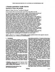
n o MCMC: posterior sample α∗i for i = 1, 2, . . . , 10, 000 o n Gives θ∗125,i = x T125 α∗i , i = 1, 2, . . . , 10, 000 θ∗125,i ∼˙ 0.248 ± 0.072 General accuracy formula: Other subjects


ˆ = 0.248 frequentist sd 0.071 for E

freq sd < Bayes sd


9 / 30

400 300 0

100

200

Frequency

500

600

700

Figure 2. 10000 MCMC values for Theta =Subject 125 estimate; mean=.248, stdev=.0721; Frequentist Sd for E{theta|data} is .0708, giving Coefficient of Variation 29%

^

[ 0.0

0.1

0.2

^

]

●

.248 0.3

0.4

0.5

MCMC mu125 values



10 / 30

Posterior CDF of θ125

n o Apply GAC to si∗ = I ti∗ < c so E{s|data} = Pr{θ125 ≤ c|data} c = 0.3 :


ˆ = 0.762 ± 0.304 E % % Bayes GAC sd estimate


11 / 30

0.6 0.4 0.0

0.2

Prob{mu125 < c | data}

0.8

1.0

Figure 3. MCMC posterior cdf of mu125, Diabetes data, Prior exp{−.37*L1(alpha)}; verts are +− One Frequentist Standard Dev

[

●

]

.336

0.0

0.1

0.2

0.3

0.4

c value Upper 95% credible limit is .336 +− .071



12 / 30

Exponential Families

Tˆ fα βˆ = e α β−ψ(α) f0 βˆ

“x”= βˆ and “µ”= α

General Accuracy Formula n o ˆ = E t(α) βˆ For E

α = αx (µ)

1/2 b = cov t, α βˆ T Vαˆ cov t, α βˆ sd n o ¨ α). with Vαˆ = covα=ˆα βˆ = ψ(ˆ



13 / 30

Bayesian Estimation Using the Parametric Bootstrap Efron (2012)

n o Parametric bootstrap: fαˆ (·) → βˆ∗1 , βˆ∗2 , . . . , βˆ∗B n o ˆ = E t(α) βˆ for prior π(α) Want to calculate: E Importance sampling: ˆ E

B X

ti πi Ri

1

ˆ∗i , πi = π α ˆ∗i , ti = t α

and

,X B

πi Ri

1

Ri = “conversion factor”

Ri = fαˆ∗i βˆ fαˆ βˆ∗i (Easy in exponential families.) Bradley Efron (Stanford University)


14 / 30

Bootstrap for GAC

.P B pi = πi Ri 1 πj Rj is weight on ith Bootstrap Replication ˆ = PB pi t ∗ E i=1 i PB ˆ estimates cov α, t βˆ ˆ∗i ti∗ − E cd ov = i=1 pi α 1/2 T b d d sd = cov Vαˆ cov



15 / 30

Prostate Cancer Study Singh et al. (2002)

Microarray study: 102 men — 52 prostate cancer, 50 healthy controls 6033 genes zi test statistic for H0i : “no difference” H0i : zi ∼ N(0, 1) Goal:

identify genes involved in prostate cancer



16 / 30

200 100

Frequency

300

400

Figure 4. Prostate study: 6033 z−values and matching N(0,1) density

0

●

3 −4

−2

0

2

4

z value



17 / 30

Poisson GLM

Histogram:

49 bins, cj midpoint of bin j

yj = #{zi in bin j} Poisson GLM:

ind

yj ∼ Poi(µj ) log(µ) = poly(c, degree=8)

[MLE:

glm(y ∼ poly(c,8), Poisson)]



18 / 30

Bayesian Estimation for the Poisson Model

Model: Prior: cdf:

y ∼ Poi(µ),

µ = eX α

[X = poly(c,8)]

Jeffreys prior for α α → µ → cdf: Fα (z) =

X

µi

,X

µi

ci ≤z

Fdr parameter: t(α) =

1 − Φ(3) = Fdr(3) 1 − F(3)

[MLE: Fdrαˆ (3) = 0.183]



19 / 30

5

density

10

15

Figure 5. Prostate study: posterior density for Fdr(3) based on 4000 parametric bootstraps from Poisson poly(8) gave posterior (m,sd) =(.183,.025); Frequentist Sd for .183 equalled .026; CV=14%

0

●

E{t|x}=.183 0.15

0.20

0.25

0.30

Fdr(3) values Internal coefficient of variation = .0023



20 / 30

Model Selection Calculations

Full model:

y ∼ Poi(µ),

Submodel Mm :

µ = eX α

i h α ∈ R9 , µ ∈ R49

{µ : only 1st m + 1 coordinates of β , 0}

Bayesian model selection:

prior probabilities on

and within each Mm Poor man’s model estimates:

partition R49 into

“preference regions“ Rm = {µ closest to Mm } Calculate posterior probabilities Pr{Rm |y}



21 / 30

Posterior Model Probabilities

Distance:

minimum AIC from µ to point in Rm

Preferred model:

is one with smallest distance

Rm

4

5

6

7

8

posterior prob

.36

.12

.05

.02

.45

sd

.32

.16

.08

.03

.40



22 / 30

Empirical Bayes Accuracy zk = observed value for gene k θk = “true effect size” zk ∼ N(θk , 1) Unknown prior g(·) → θ1 , θ2 , . . . , θN

[N = 6033]

From observations z1 , z2 , . . . , zN we wish to estimate ,Z Z Ez = E t(θ) z = t(θ)fθ (z)g(θ) dθ fθ (z)g(θ) dθ [if t(θ) = δ0 (θ) then Ez = Pr{θ = 0|z}]. Bradley Efron (Stanford University)


23 / 30

Parametric Families of Priors p-parameter exponential family: log gα (θ) = q(θ)T α + constant 1×p

p×1

α the unknown parameter R Marginal: fα (z) = fθ (z)gα (θ) dθ T e.g., q(θ) = δ0 (θ), θ, θ2 , θ3 , θ4 , θ5

[“spike and slab”] marginal MLE

ˆ α → gα → fα → (z1 , z2 , . . . , zN ) −→ α .R R ˆ z = t(θ)fθ (z)gαˆ (θ) dθ fθ (z)gαˆ (θ) dθ ±?? E MLE:



24 / 30

ˆz Delta-Method Standard Deviation of E ( )1/2 dEz T −1 dEz ˆ Iα sd Ez = dα dα Fisher information matrix:

I I

¯α = q

R

q(θ)gα (θ) dθ R ¯ ] dθ hα (z) = fθ (z)gα (θ) [q(θ) − q

Z Iα = N

hα (z)hα (z)T dz fα (z)

R dEz ¯ ] dθ where = Ez w(θ)gα (θ) [q(θ) − q dα .R .R w(θ) = t(θ)fθ (z)gα (θ) tfgα − fθ (z)gα (θ) fgα Bradley Efron (Stanford University)


25 / 30

0.6 0.4

●

0.0

0.2

prob{|theta| >2|z}

0.8

1.0

Figure 6. Estimated prob{abs(theta)>2 | z value} Prostate study; Bars show +− one freq stdev. Using g−model {0,ns(5)}

●

3 −4

−2

0

2

4

6

z value Prob{abs(theta)>2 | z=3} = .434 +− .071



26 / 30

Estimated False Discovery Rate

Local false discovery rate:

fdr(z) = Pr {θ = 0|z} = E t(θ)|z

where t(θ) = δ0 (θ) Next:

applied to prostate study



27 / 30

0.6 0.4

prob{theta=0|z}

0.8

1.0

Figure 7. Estimated prob{theta=0 | z value} Prostate study; Bars show +− one freq stdev. Using g−model {0,ns(5)}

0.0

0.2

●

●

3 −4

−2

0

2

4

6

z value Prob{theta=0 | z=3} = .322 +− .068, coeff of var =.21



28 / 30

For z = 3:

b {|θ| > 2|z = 3} = 0.43 ± 0.07 Pr c fdr(3) = 0.32 ± 0.07 “locfdr”:

c exfam modeling of z’s, not θ’s, gave fdr(3) = 0.35 ± 0.03

but doesn’t work for |θ| > 2, etc.



29 / 30

References

Park and Casella (2008) “The Bayesian Lasso” JASA 681–686 Singh et al. (2002) “Gene expression correlates of clinical prostate cancer behavior” Cancer Cell 203–209 Efron, Hastie, Johnstone and Tibshirani (2004) “Least angle regression” Ann. Statist. 407–499 Efron (2012) “Bayesian inference and the parametric bootstrap” Ann. Appl. Statist. 1971–1997 Efron (2010) Large-Scale Inference: Empirical Bayes Methods for Estimation, Testing, and Prediction IMS Monographs, Cambridge University Press



30 / 30