N00014-93-1-0385 and contract No. N00014-95-1-0600. Partial support was also provided by Daimler-Benz AG, Eastman Kodak, Siemens Corporate Research ...
MASSACHUSETTS INSTITUTE OF TECHNOLOGY ARTIFICIAL INTELLIGENCE LABORATORY and
CENTER FOR BIOLOGICAL AND COMPUTATIONAL LEARNING DEPARTMENT OF BRAIN AND COGNITIVE SCIENCES A.I. Memo No. 1649 C.B.C.L Paper No. 166
November 1998
From Regression to Classification in Support Vector Machines Massimiliano Pontil, Ryan Rifkin and Theodoros Evgeniou This publication can be retrieved by anonymous ftp to publications.ai.mit.edu. The pathname for this publication is: ai-publications/1500-1999/AIM-1XXX.ps Abstract We study the relation between support vector machines (SVMs) for regression (SVMR) and SVM for classification (SVMC). We show that for a given SVMC solution there exists a SVMR solution which is equivalent for a certain choice of the parameters. In particular our result is that for � sufficiently close to one, the optimal hyperplane and threshold for 1 times the optimal the SVMC problem with regularization parameter Cc are equal to 1−� hyperplane and threshold for SVMR with regularization parameter Cr = (1−�)Cc . A direct consequence of this result is that SVMC can be seen as a special case of SVMR. c Massachusetts Institute of Technology, 1998 Copyright � This report describers research done at the Center for Biological & Computational Learning and the Artificial Intelligence Laboratory of the Massachusetts Institute of Technology. This research was sponsored by the Office of Naval Research under contract No. N00014-93-1-0385 and contract No. N00014-95-1-0600. Partial support was also provided by Daimler-Benz AG, Eastman Kodak, Siemens Corporate Research, Inc., and AT&T.
1
Introduction
We assume that the reader has some familiarity with Support Vector Machines. In this section, we provide a brief review, aimed specifically at introducing the formulations and notations we will use throughout this paper. For a good introduction to SVMs, see [1] or [2]. In the support vector machine classification problem, we are given l examples (x1 , y1), . . . , (xl , yl ), with xi ∈ R n and yi ∈ {−1, 1} for all i. The goal is to find a hyperplane and threshold (w, b) that separates the positive and negative examples with maximum margin, penalizing points inside the margin linearly in a user-selected regularization parameter C > 0. The SVM classification problem can be restated as finding an optimal solution to the following quadratic programming problem: (C)
min w, b, ξ
1 �w�2 2
+C
��
i=1 ξi
yi(w · xi + b) ≥ 1 − ξi ξ ≥0
i = 1, . . . , l
This formulation is motivated by the fact that minimizing the norm of w is equivalent to maximizing the margin; the goal of maximizing the margin is in turn motivated by attempts to bound the generalization error via structural risk minimization. This theme is developed in [2]. In the support vector machine regression problem, the goal is to construct a hyperplane that lies “close” to as many of the data points as possible. We are given l examples (x1 , y1), . . . , (xl , yl ), with xi ∈ R n and yi ∈ R for all i. Again, we must select a hyperplane and threshold (w, b)1 . Our objective is to choose a hyperplane w with small norm, while simultaneously minimizing the sum of the distances from our points to the hyperplane, measured using Vapnik’s �-insensitive loss function: �
|yi − (w · xi + b)|� =
0 if |yi − (w · xi + b)| ≤ � |yi − (w · xi + b)| − � otherwise
(1)
The parameter � is preselected by the user. As in the classification case, the tradeoff between finding a hyperplane with small norm and finding a hyperplane that performs regression well is controlled via a user selected regularization parameter C. The quadratic programming problem associated with SVMR is: (R)
min w, b, ξ, ξ ∗
1 �w�2 2
+C
��
i=1 (ξi
+ ξi∗ )
yi − (w · xi + b) ≤ � + ξi −yi + (w · xi + b) ≤ � + ξi∗ ξ, ξ ∗ ≥ 0
i = 1, . . . , l i = 1, . . . , l
The main aim of this paper is to demonstrate a connection between support vector machine classification and regression. In general, SVM classification and regression are performed using a nonlinear kernel K(xi , xj ). For simplicity of notation, we chose to present our formulations in terms of a linear separating hyperplane w. All our results apply to the nonlinear case; the reader may assume that we are trying to construct a linear separating hyperplane in a high-dimensional feature space. 1
Observe that now the hyperplane will reside in n + 1 dimensions.
1
2
From Regression to Classification
In the support vector machine regression problem, the yi are real-valued rather than binaryvalued. However, there is no prohibition against the yi being binary-valued. In particular, if yi ∈ {−1, 1} for all i, then we may perform support vector machine classification or regression on the same data set. Note that when performing support vector machine regression on {−1, 1}-valued data, if � ≥ 1, w = 0, ξ = 0, ξ ∗ = 0 is an optimal solution to R. Therefore, we restrict our attention to cases were � < 1. Loosely stated, our main result is that for � sufficiently close to one, the optimal hyperplane and threshold for the support vector machine classification problem with 1 times the optimal hyperplane and threshold for the regularization parameter Cc are equal to 1−� support vector machine regression problem with regularization parameter Cr = (1 − �)Cc . We now proceed to formally derive this result. We make the following variable substitution: �
ηi =
ξi if yi = 1 ξi∗ if yi = −1.
�
, ηi∗ =
ξi∗ if yi = 1 ξi if yi = −1.
(2)
Combining this substitution with our knowledge that yi ∈ {−1, 1} yields the following modification of R: (R� )
1 �w�2 2
min w, b, η, η ∗
+C
��
i=1 (ηi
+ ηi∗ )
yi (w · xi + b) ≥ 1 − � − ηi yi (w · xi + b) ≤ 1 + � + ηi∗ η, η ∗ ≥ 0
i = 1, . . . , l i = 1, . . . , l
Continuing, we divide both sides of each constraint by 1 − �, and make the variable substitutions � η η∗ w b w� = 1−� , b� = 1−� , η � = 1−� , η ∗ = 1−� : (R�� )
1 �w� �2 2
min � � � w , b , η �, η ∗
+
C �� ( i=1 (ηi� 1−�
�
+ ηi∗ ))
yi(w� · xi + b) ≥ 1 − ηi� i = 1, . . . , l 1+� � ∗� yi(w · xi + b) ≤ 1−� + ηi i = 1, . . . , l � η�, η∗ ≥ 0 Looking at formulation R�� , one suspects that as � grows close to 1, the second set of constraints will be “automatically” satisfied with η ∗ = 0. We confirm this suspicion by forming the Lagrangian dual: (RD�� ) min β
1 2
�l
i,j=1 (βi
�
− βi∗ )Dij (βi − βi∗ ) −
� i
�
βi +
1+� 1−�
� i
βi∗
yi βi = i yi βi∗ βi , βi∗ ≥ 0 C βi , βi∗ ≤ 1−� where D is the symmetric positive semidefinite matrix defined by the equation Dij ≡ yi yj xi xj . For all � sufficiently close to one, the ηi∗ will all be zero: to see this, note that η = 0, η ∗ = 0 is a feasible solution to RD�� with cost zero, and if any ηi∗ is positive, for � sufficiently close to one, the value of the solution will be positive. Therefore, assuming that � is sufficiently large, we may i
2
eliminate the η ∗ terms from R�� and and the β ∗ terms from D�� . But removing these terms from R�� leaves us with a quadratic program essentially identical to the dual of formulation C: (CD�� ) min β
1 2
�l
i,j=1 βi Dij βj
� i
−
�
i
βi
yi βi = 0 βi ≥ 0 C βi ≤ 1−�
Going back through the dual, we recover a slightly modified version of C: C �� (C � ) min 12 �w�2 + 1−� i=1 ξi w, b, ξ yi (w · xi + b) ≥ 1 − ξi i = 1, . . . , l ξ ≥0 Starting from the classification problem instead of the regression problem, we have proved the following theorem: Theorem 2.1 Suppose the classification problem C is solved with regularization parameter C, and the optimal solution is found to be (w, b). Then, there exists a value a ∈ (0, 1) such that ∀� ∈ [a, 1), if problem R is solved with regularization parameter (1 − �)C, the optimal solution will be (1 − �)(w, b). Several points regarding this theorem are in order: • The η substitution. This substitution has an intuitive interpretation. In formulation R, a variable ξi is non-zero if and only if yi lies above the �-tube, and the corresponding ξi∗ is non-zero if and only if yi lies below the �-tube. This is independent of whether yi is 1 or −1. After the η substitution, ηi is non-zero if yi = 1 and yi lives above the �-tube, or if yi = −1 and yi lives below the �-tube. A similar interpretation holds for the ηi∗ . Intuitively, the ηi correspond to error points which lie on the same side of the tube as their sign, and the ηi∗ correspond to error points which lie on the opposite side. We might guess that as � goes to one, only the former type of error will remain: the theorem provides a constructive proof of this conjecture. • Support Vectors. Examination of the formulations, and their KKT conditions, shows that there is a one-to-one correspondence between support vectors of C and support vectors of R under the conditions of correspondence. Points which are not support vectors in C and therefore lie outside the margin and are correctly classified will lie strictly inside the �-tube in R. Points which lie on the margin in C will lie on the boundaries of the �-tube in R, and are support vectors for both problems. Finally, points which lie inside the margin or are incorrectly classified in C will lie strictly outside the �-tube, above the tube for points with y = 1, below the tube for points with y = −1, and are support vectors for both problems. • Computation of a. Using the KKT conditions associated with problem (R�� ), we can determine the value of a which satisfies the theorem. To do so, simply solve problem C � , and � choose a to be the smallest value such that when the constraints (w� · xi +b) ≤ 1+� +ηi∗ , i = 1−� 1, . . . , l are added, they are satisfied by the optimal solution to C � . In particular, if we define m to be the maximal value of yi (w · xi + b), then a = m−1 will satisfy the theorem. Observe m+1 that as w := �w� gets larger (i.e., the separating hyperplane gets steeper), or as the 3
correctly classified xi get relatively (in units of the margin w −1 ) farther away from the hyperplane we expect a to increase. More precisely it is easy to see that m ≤ wD, with D the diameter of the smallest hypersphere containing all the points. Then a ≥ wD−1 , which wD+1 is an increasing function of w. Finally observe that incorrectly classified points will have yi (w · xi + b) < 0, and therefore they cannot affect m or a. • The ξ 2 case. We may perform a similar analysis when the slack variables are penalized quadratically rather than linearly. The analysis proceeds nearly identically. In the transition from formulation R� to R�� , an extra factor of (1 − �) falls out, so the objective � � function in R�� is simply 12 �w��2 + C( �i=1 ((ηi� )2 + (ηi∗ )2 )). The theorem then states that for sufficiently large �, if (w, b) solves C with regularization parameter C, (1 − �)(w, b) solves R, also with regularization parameter C.
3
Examples
In this section, we present two simple one-dimensional examples that help to illustrate the theorem. These examples were both performed penalizing the ξi linearly. In the first example, the data are linearly separable. Figure 1a shows the data points, and Figure 1b shows the separating hyperplane found by performing support vector classification with C = 5 on this data set. Note that in the classification problem, the data lie in one dimension, with the y-values being “labels”. The hyperplane drawn shows the value of w · x + b as a function of x. The computed value of a is approximately .63. Figure 1c shows the �-tube computed for the regression problem with � = .65, and Figure 1d shows the same for � = .9. Note that every data point is correctly classified in the classification problem, and that every data point lies inside the �-tube in the regression problems, for the values of � chosen. In the second example, the data are not linearly separable. Figure 2a shows the data points. Figure 2b shows the separating hyperplane found by performing classification with C = 5. The computed value of a is approximately .08. Figures 2c and d show the regression tubes for � = .1 and � = .5, respectively. Note that the points that lie at the edge of the margin for classification, x = −5 and x = 6 lie on the edge of the �-tube in the regression problems, and that points that lie inside the margin, or are misclassified, lie outside the �-tube. The point x = −6, which is the only point that is strictly outside the margin in the classification problem, lies inside the �-tubes. The image provides insight as to why a is much smaller in this problem than in the linearly separable example: in the linearly separable case, any �-tube must be shallow and wide enough to contain all the points.
4
Conclusions and Future Work
In this note we have shown how SVMR can be related to SVMC. Our main result can be summarized as follows: if � is sufficiently close to one, the optimal hyperplane and threshold 1 for the SVMC problem with regularization parameter Cc are equal to 1−� times the optimal hyperplane and threshold for SVMR with regularization parameter Cr = (1 − �)Cc . A direct consequence of this result is that SVMC can be regarded as a special case of SVMR. An important problem which will be study of future work is whether this result can help place SVMC and SVMR in the same common framework of structural risk minimization. 4
1 1 0.8 0.8 0.6
0.6
0.4
0.4
0.2
0.2
0
0
−0.2
−0.2 −0.4
−0.4
−0.6
−0.6
−0.8 −0.8 −1 −1 −6
−4
−2
0
2
4
6
−6
−4
(a) Data
−2
0
2
4
6
4
6
(b) Classification
1
1
0.8
0.8
0.6
0.6
0.4
0.4
0.2
0.2
0
0
−0.2
−0.2
−0.4
−0.4
−0.6
−0.6
−0.8
−0.8
−1
−1
−6
−4
−2
0
2
4
6
−6
(c) Regression, � = .65
−4
−2
0
2
(d) Regression, � = .9
Figure 1: Separable data.
5
Acknowledgments
We wish to thank Alessandro Verri, Tomaso Poggio, Sayan Mukherjee and Vladimir Vapnik for useful discussions.
References [1] C. Burges. A tutorial on support vector machines for pattern recognition. In Data Mining and Knowledge Discovery, volume 2, pages 1 – 43. Kluwer Academic Publishers, Boston, 1998. [2] V. Vapnik. Statistical Learning Theory. John Wiley and sons, New York, 1998.
5
1 1 0.8 0.8 0.6
0.6
0.4
0.4
0.2
0.2
0
0
−0.2
−0.2 −0.4
−0.4
−0.6
−0.6
−0.8 −0.8 −1 −1 −6
−4
−2
0
2
4
6
−6
−4
(a) Data
−2
0
2
4
6
4
6
(b) Classification
1
1
0.8
0.8
0.6
0.6
0.4
0.4
0.2
0.2
0
0
−0.2
−0.2
−0.4
−0.4
−0.6
−0.6
−0.8
−0.8
−1
−1
−6
−4
−2
0
2
4
6
−6
(c) Regression, � = .1
−4
−2
0
2
(d) Regression, � = .5
Figure 2: Non-separable data.
6