Sumbangan Baja*; David M. Chapman; and Deirdre Dragovich. Division of ......
International Journal of Geographic Information Systems, vol.8, no. 4, Nov, pp.
Fuzzy Modelling Of Environmental Suitability Index For Rural Land Use Systems: An Assessment Using A GIS Sumbangan Baja*; David M. Chapman; and Deirdre Dragovich Division of Geography, School of Geosciences, The University of Sydney NSW 2006, Australia; ph +61-2-93514589, fax +61-2-93513644 (*corresponding author, email:
[email protected]) Abstract. The increasing use and capability of geocomputation tools, as well as increasing availability of land resource information, offer opportunities to utilise such tools for the effective management of information for planning purposes. One among those is the development of spatially-based models that may be used for efficiently undertaking land suitability assessment based on available information. This paper presents a spatial modelling procedure for the assessment of land suitability using geographical information systems (GIS). The model consists of two sub-models: land suitability indexing and erosion tolerance indexing. Both were modelled based on fuzzy set methodology in a GIS. A soil landscape map (scale 1:100 000), complemented by New South Wales SALIS (Soil And Land Information System), was used in conjunction with a Digital Elevation Model (DEM) to derive a land suitability index (LSI) for cropping. An erosion tolerance index (ETI) was established from the integration of soil loss tolerance (T-value) and average annual soil loss (A) estimated using the Revised Universal Soil Loss Equation (RUSLE). An environmental suitability index (ESI) was then generated from a convex combination of LSI and ETI. The available land capability map (scale 1:25 000) produced by NSW Soil Conservation Service was employed for cross-checking with the model outputs. It was found that the outputs are consistent with that land capability classification scheme. A sensitivity analysis also reveals reasonably good results. The procedures developed show the significance of this model for the basis of identifying and delineating land management units at a detailed scale.
1.
INTRODUCTION
Appropriate land use decisions are vital to achieve optimum productivity of the land and to ensure environmental sustainability. This requires an effective management of land information on which such decisions should be based. Land suitability evaluation is one of the effective tools for such purposes. Land suitability evaluation, commonly known as ‘land evaluation’, may be defined as ‘the process of assessment of land performance when the land is used for specified purpose’ (FAO, 1985). There are two general kinds of land suitability evaluation approaches: qualitative and quantitative. A qualitative approach is used to assesses land potential at a broad scale, or employed as a preliminary to more detailed investigations (Dent and Young, 1981). The results of classification are generally given in qualitative terms only, such as highly suitable, moderately suitable, and not suitable. The second approach is that using parametric techniques involving more detailed land attributes which allow various statistical analyses to be performed. In a parametric-quantitative approach, the evaluation procedure generally involves deductive, inductive or simulation modeling systems (Shields et al., 1996; van de Graaff, 1988) to quantify the potential of land for specific uses. A deductive approach deals mainly with the estimated yield as an index relative to a standard yield (Soil Survey Staff, 1951), while an inductive
technique utilizes land characteristics as evaluation criteria to establish land unit indices. This latter approach involves such arithmetical operations as additive (Moss, 1972), multiplicative (Pierce et al., 1983; Storie, 1978; Sys, 1985), and complex (Karlen and Stott, 1994). Simulation modelling uses a complex of multivariate factors, and makes use of a computerbased analysis system such as an expert system (see for example Johnson and Cramb, 1991). Such kinds of approaches have recently been widely used and developed with the aid of GIS-based systems (see for example Beinroth et al., 1998). Use of a fuzzy set methodology (Burrough, 1989; Burrough et al, 1992; Tang and van Ranst, 1992; Wang et al., 1990) has made a significant contribution to the refinement of land suitability analyses. Land evaluation is a tool to ‘predict land performance, both in terms of the expected benefits from and constraints to productive land use, as well as the expected environmental degradation due to these uses’ (Rossiter, 1996). Therefore, for land to be suitable (for a given purpose) and for the use to be sustainable, it must address the values that are related to both aspects: degree of suitability, and potential degradation (from long-term perspective) resulting from land management practices. This paper presents a spatiallybased model of land suitability analysis that considers both aspects of land evaluation. The main purpose is to establish indices of environmental suitability for cropping land use systems. A fuzzy set methodology was employed in the modelling procedures, and a GIS
was used to facilitate every stage of the modelling processes. In the sections that follow, a brief overview on fuzzy sets is presented, followed by descriptions of the model framework and methodology in separate sections. The results of modelling procedures are then presented together with uncertainty and sensitivity analysis, before presenting discussion and conclusion. 2.
FUZZY SETS AND MEMBERSHIP FUNCTIONS
A fuzzy set is most commonly used for classifications of objects or phenomena in continuous values, where the classes do not have sharply defined boundaries. It deals with a class with a continuum of grades of memberships (Zadeh, 1965). A fuzzy set A may be defined as follows: A = {x, µA(x)} x ε X ………………….………….(1) Where X = {x} is a finite set (or space) of objects or phenomena, µA(x) is a membership function of X for subset A Therefore, a fuzzy subset is defined by the membership function (MF) that defines the membership grades of fuzzy objects or phenomena in the ordered pairs, consisting of the objects and their membership grades. The MF of a fuzzy subset determines the degree of membership of x in A (Burrough, 1989). There are several ways to generate a fuzzy membership function. For environmental applications, there are two different but complementary approaches to grouping individuals into fuzzy sets or classes (McBratney and Odeh, 1997). The first is the Similarity Relation model (SR), and the second is based on the Semantic Import model (SI). The fuzzy c-means and its modifications (see e.g., McBratney and Gruijter, 1992) is one of the examples for the first. An SI model (see Burrough, 1989) is comparatively simple to use, because it utilizes an a priori membership function (MF) for individual variables under consideration (Burrough, 1989). Examples can be seen in Burrough (1989), Burrough et al. (1992), and Davidson et al. (1994). With this approach, the attribute values considered are converted to common membership grades (from 0 to 1.0), according to the class limits specified by the analysts based on experience or conventionally imposed definitions (McBratney and Odeh, 1997). If MF(xi) represents individual MF values for ith land property x, then, the basic SI model function take the following form in the computation process: MF(xi) = [1/(1 + {(xi – b)/d}2)]………………….. (2) As there are n land characteristics to be rated, the MF values of individual land characteristics under consideration are then combined using a convex combination function to produce a join membership function (JMF) of all attributes, Y as follows: n
JMF(Y) =
Σλ MF(x ) i
i
.….....……....…..…… (3)
i=1
where λi is a weighting factor for the ith land property x, and MF(xi) denotes a membership grade for the ith land property x. 3.
MODEL FRAMEWORK
3.1 Model structures and components There are three sets of model components used in establishing an environmental suitability index (ESI): (i) land use scenarios (including types of management/ support practices); (ii) requirements/ limitations; and (iii) operational functions and databases in GIS. As seen in Figure 1, types of requirements/ limitations (biophysical land properties) and land management/ support practices depend on the selected land use (scenario). For instance, if cropping is selected as a land use scenario, then requirements will include a set of information such as physical and chemical properties of soils, topography, and climate. Combinations and ratings of such factors, in a certain way, are then used to produce a land suitability index (LSI). Such a strategy is commonly known as land suitability evaluation (FAO, 1976). Further, information on land management practices, including erosional control strategies to be applied, is also necessary, as one of the determinants of possible land degradation. Complemented with an assessment of soil loss tolerance (T-value), such information will then become the basis of calculating an erosion tolerance index (ETI). Integration of LSI and ETI gives rise to an environmental suitability index (ESI) for the selected type of land use and land management practices. The second component of the model is land use requirements on which decision criteria are based. The databases used are formed and structured according to such requirements. In a GIS environment, there are two types of spatial data structure: raster and vector. The primary theoretical difference between the two data structures is that the raster structure stores information on the interior of areal features and implies boundaries; whereas the vector structure stores information about boundaries, and implies interiors (Berry, 1988). In a vector program such as Arc/Info, feature attributes are stored in the polygon attribute table (PAT) and arc attribute table (AAT) files for polygon and arc layers, respectively. The model presented here makes use of both data structures. Final computation of ESIs was done in a raster format, involving data conversion procedures from vector to raster. As seen in Figure 1, operations and functions, which are symbolised with ellipses, were undertaken in vector (PC-based Arc/Info) and raster (IDRISI 32) formats. There are three basic groups of operations in performing computations: (i) fuzzy set functions; (ii) convex combination; (iii) multiplication. The first and second belong to operation in SI-based fuzzy set
methodology, while multiplication function also includes the Revised Universal Soil Loss Equation (RUSLE) (Renard et al., 1997). They are described in the sections that follow. Land use scenarios Requirements/ limitations
Soil landscapes
DEM
Soil attribu tes
Individual MFs
Rainfall Management/ conservation
Slope
Fuzzy s et function
(gradient, length)
RUSLE Soil attribu tes
Indiv idual MFs
Convex combination
Potential erosion
JMF Slope
JMF Soils
[JMF(T)]
[J MF(S)]
LSIs = J MF(S) x JM F(T)
Annual soil loss (A) T-value
Land Suitability Indices (LSIs)
T/A ratio Fuzzy set function
Convex combination
Erosion Tolerance Indices (ETIs)
Environme nta l Suitabil ity Indices (ESIs)
Figure 1: A general scheme of the model developed
3.2 Model functions for fuzzy membership classification Model functions used for fuzzy membership classification of land attributes are based on the SI approach, which utilises a bell-shaped curve (Burrough et al., 1992). This approach consists of two basic functions: symmetric and asymmetric. The first function, also called an ‘optimum range’ (see Wymore, 1993), distinguishes two variants: one that uses a single ideal point (Model 1), while the other employs a range of ideal points (Model 2), as will be described later. For example, an ideal level of soil pH for agricultural purposes may range from slightly acid to slightly alkaline, and very low and very high pH values are limiting for agricultural crops. Therefore, a symmetric function with a range of ideal points (Model 2) is the one appropriate for rating soil pH for cropping. The second function, an asymmetric model, is used where only the lower and upper boundary of a class have practical importance (Burrough and McDonnell, 1998). This function consists of two variants: asymmetric left (Model 3) and asymmetric right (Model 4). For example, with regard to soil depth ‘more is better,’ so that it is appropriate to use an asymmetric left model. A similar concept applies to organic carbon content, cation exchange capacity, available water capacity, etc. With a similar rule, an asymmetric right, which is ‘less is better’ is appropriate for rating salinity, slope, erosion, percentage of stones or cobbles, etc.
In this modelling process, computation of criterion membership functions was based on equation (2), which applies to Model 1. In addition to that, the following forms also apply to Models 2, 3, and 4: For optimum range (Model 2): MF(xi) = 1 if (b 1 + d 1) < xi < (b 2 – d 2) ………….. (4) For asymmetric left (Model 3): MF(xi) = [1/(1 + {(xi – b 1 – d 1)/d 1}2)] if xi < (b 1 + d 1) .……………………………………..……..……….. (5) For asymmetric right (Model 4): MF(xi) = [1/(1 + {(xi – b 2 + d 2)/d 2}2)] if xi > (b 2 – d 2) .…….……………………..…….……………... (6) 3.3 RUSLE-based soil erosion model RUSLE (Renard et al., 1997) was used as part of the model structure to calculate potential average annual soil loss and the level of soil loss tolerance (T-value) (see Figure 1). The RUSLE program (originally, USLE) was first developed in U.S.A and was designed for use in U.S conditions. For use in New South Wales, Australia, Rosewell and Edwards (1986) developed a SOILOSS program adapting the principles of RUSLE. Although SOILOSS cannot tackle spatial data sets from a GIS, it is useful to serve as the basis for model parameterisation undertaken in the present study. RUSLE utilises an empirical equation with a multiplication function as follows (Wischmeier and Smith, 1978; Renard et al., 1997):
4. A = R x K x LS x C x P ……………………………(7) where, A denotes annual soil loss (t/ha/y), R is index of rain erosivity, K represents index of soil erodibility, LS are slope factors (L = length, and S = gradient), and C and P represent land cover and conservation practice (support) factors. Clearly, these parameters can also be extracted from the information needed for establishing requirements (or decision criteria) for a selected land use scenario (Figure 1).
4.1 Study area, data base and preliminary data processing The area selected for this study includes some parts of the lower Hawkesbury-Nepean River catchment, covering an area of approximately 370 square kilometres, located about 60 km northwest of Sydney (Figure 2). Data bases used were obtained from the following sources: •
Soil landscape map series, Penrith, scale 1 : 100,000 (Bannerman and Hazelton, 1990)
•
SALIS (Soil And Land Information System) held in the Department of Land and Water Conservation (DLWC), New South Wales
•
A three-second Digital Elevation Model
•
Climate data (rainfall erosivity)
3.4 Soil loss tolerance Soil loss tolerance (or T-value) is defined as ‘the maximum rate of soil erosion that permits an optimum level of crop productivity to be sustained economically and indefinitely’ (ISSS, 1996). It is also sometimes called permissible soil loss (Kok et al., 1995) which is related to the average annual soil loss a given soil type may experience and still maintain its productivity over an extended period of time. In many situations, the establishment of a T-value is intended to provide basic information for the maintenance of soil productivity, which becomes one of the foci of sustainability of agricultural land use (Smith and McDonald, 1998). Therefore, T-values may be determined based on the factors affecting long-term productivity. For practical purposes, T-values may be estimated based on favourable rooting depth (McCormack et al., 1982). The generally accepted maximum limit of soil loss (or Tvalue) is 11.2 t/ha/y (Wischmeier and Smith, 1978), while Rubio (1986) considered a T-value of 20 t/ha/y. An average soil loss of 5 t/ha/y has been considered as the limit for shallow soils (Hudson, 1986). Lal (1985) observed that for shallow soils with root-restrictive layers at 0.2 to 0.3 m depth, a T-value is set at 1 t/ha/y. A comprehensive guideline for the estimation of Tvalues based on the favourable rooting depth can be found in USDA-SCS (1973). Furthermore, for general purposes DLWC (1997) outlined a recommended maximum acceptable soil loss for agricultural and forestry areas in New South Wales, with three different ranges of soil depth, as follows: •
For deep soils (>1.5 m), T-value is set to 10 t/ha per year
•
For moderately thick soils (1.0 – 1.5 m), T-value is set to 5 t/ha per year
•
For shallow soils (< 1.0 m), T-value is 1 t/ha per year.
METHODOLOGY
Soil landscape boundaries were digitised in Arc/Info, and attribute data were input in the polygon attribute (PAT) files. A DEM was available in raster format, and the IDRISI 32 program was used to handle all raster data. Five types of landscapes were found in the study area and these were further divided into seventeen different soil landscapes (Table 1).
Aust ral ia
New South Wales
N
Bro ken Bay
Study area 0
1 0k m
Winds or Ric hmond
Penrith Po rt Ja ckso n
Liv er pool
Sy dney CBD Bo ta ny Bay Bate Bay
Figure 2: Site location of study area Table 1: Soil landscapes in the study area Landscapes
Residual
Estimation of T-values in this study was based on both guidelines (USDA-SCS, 1973; DLWC, 1997). Colluvial
Erosional
Soil landscapes Faulconbridge (fb) Lucas Heights (lh) Blacktown (bt) Kurrajong (kj) Volcanic (vo) Warragamba (wb) Hawkesbury (ha) Picton (pn) Gymea (gy)
Fluvial
Aeolian/alluvial
unit of individual properties in the spatial representation of membership function (MF) and joint membership function (JMF) of soil attributes.
Luddenham (lu) Woodlands (wl) South Creek (sc) Freemans Reach (fr) Richmond (ri) Upper Castlereagh (up) Berkshire Park (bp) Agnes banks (ab)
In the computation, it is crucial to examine an appropriate SI model parameter to suit each decision criterion. The choice depends on the ‘trend of performance’ of the respective land attribute in accommodating a favourable condition for a selected land use type (Baja et al., 2001). Model parameters seen in Table 2 include LCP (lower crossover point), b (central concept), UCP (upper crossover point), and d (width of transition zone) (see Burrough et al., 1992). LCP and UCP represent the situation where a land attribute examined is at a marginal level for a given purpose, while b is for an ideal level (see Sys, 1985). For example, available water capacity (AWC), presented as a cardinal form, C (Table 2), takes an asymmetric left function (i.e., Model 3) or more is better, because the quality function of land performs better, as the AWC level increases. The optimum AWC value (ideal, b) was set at 20%, following the ‘Productivity Index’ model developed by Pierce et al. (1983), while LCP (marginal) was set at 12.5% (Figure 3.a).
4.2 Land use, decision criteria and model parameters In the application of the present model, a land use scenario for cropping in general was chosen. Two groups of land properties were used as decision criteria for this analysis: one for LSIs, and the other for ETIs. For LSIs, as many as ten land attributes were selected as evaluation criteria (Table 2) (adapted from Sys, 1985; Zhang, 1989). The criteria for ETIs include those mentioned in equation (7), in addition to the parameters required for establishing a T-value, as will be described later.
As soil data sets were stored in an Arc/Info vector format, calculation of a membership function of each soil characteristic was done in the attribute file (PAT). Therefore, a soil landscape unit is used as a delineation Table 2: Evaluation criteria suitability assessment for cropping and selected types of fuzzy set models and MF parameters Type of Data #
Land properties
Model function
LCP
MF parameters for cropping b UCP d
Weight (2FD)
Soils Available water capacity, AWC (%) C 3 12.5 20 7.5 0.095 Site drainage [O, 5] 4 1 3 2 0.190 Texture and structure* [O, 5] 3 3 1 2 0.190 Cobbles, boulders, and stones (CBS) [O, 5] 4 1 3 2 0.095 Solum depth [O, 5] 3 3 5 2 0.190 Cation exchange capacity, CEC [O, 5] 3 2 4 2 0.048 (topsoil) Organic carbon, OC (topsoil) [O, 5] 3 3 5 2 0.048 Soil pH C 2 4.75 5.5-8.0 8.8 0.85 0.048 Salinity, Electrical Conductivity (EC) [O, 5] 4 1 2 1 0.190 Topography Slope gradient (%) C 4 2 12.5 10.5 Note: # C = cardinal; O = ordinal. [O, 5] means ordinal data with 5 categories: 1, 2, 3, 4, and 5 (Table 3), used for deriving MF *MF for texture and structure were determined based on ranking, from 1 (very poor) to 5 (very good) (Table 2)
Table 3: Categorical rankings of land attributes measured in an ordinal scale Ordinal/categorical rankings Land attributes CEC (me%) OM (%) Salinity, EC (dS/m) Drainage class Solum depth (m) CBS Soil texture and structure*
1
2
3
4
5
Very low 40 > 5.0 > 8.0
Well Very shallow < 0.15 Absent Very poor
Moderately well Shallow 0.15 – 0.4 Few Poor
Imperfect Moderate 0.4 – 0. 7 Frequent Moderate
Sm
S
Poor Very poor Slightly deep Deep 0.7 – 1.0 > 1.0 Common Abundant Good Very good SCL, SCm, ZCm, Z, ZL, ZCL, ZCs, HCm, SL, SCLm, Cm, HCs, CLm, SCs, CSs, Cs, CLs, LS CSm, Lm Ls
*C = Clay, CL= Clay loam, CS = Clayey sand, L = Loam, LS = Loamy sand, S = Sand, SC = Sandy clay, SCL = Sandy clay loam, SL = Sandy loam, Z = Silt, ZC = Silty clay, ZCL = Silty clay loam, ZL = Silt loam; Structure : s = structured, m = massive (or apedal).
Furthermore, site drainage is represented as an ordinal form (O) consisting of five categorical classes: 1, 2, 3, 4, and 5, representing well, moderately well, imperfect, poor, and very poor (Table 3). This soil property takes the form asymmetric right function (Model 4), or less is better. In other words, class 1 (well-drained soil) is more preferred to class 2 (moderately drained), and so forth. The optimum site drainage class was set at class 1, while a marginal value (LCP) was set at class 3 (Figure 3.b). The property of soil pH takes the form of a symmetric model, which presents an optimum level as a range of values (Model 2). This land characteristic, in the present study, was presented in a cardinal form (C). The optimum level (i.e., b1 and b2) was specified in the range between 5.5 and 8.0 (Table 2) (adapted from Sys, 1985; Zhang, 1989), while LCP and UCP values were set at 4.5 and 8.8 (Figure 3.c). In the study area, there is no soil landscape unit having a pH value of more than 8.0, so that only the LCP values have practical importance in the application of such a model function (Figure 3.c). Likewise, slope angle, which was derived from a DEM (in continuous-cardinal number, C) takes an asymmetric right function. An optimum slope gradient for cropping was set at 2 % or less (adapted from Sys, 1995; Zhang, 1989) (Table 2), while the UCP threshold value was specified at 12.5 % (see Figure 3.d). MF 1.0
MF b
LCP
1.0
d
0.5
b
UCP
d
0.5
weights to compute a joint membership function (JMF) of combined attributes. In the weighting procedure, the soil attributes mentioned above were grouped into three categories, ranked according to their importance in descending order: group I (soil texture and structure, effective depth, and salinity (EC)); group II (site drainage, AWC, and CBS); and group III (soil pH, OM, and CEC). Hence, attributes within each group were weighted equally. The weights as seen in Table 2 are generated based on a two-fold difference (2FD) in terms of degree of importance for the above ranked groups. Different combinations of weightings were also applied to examine the sensitivity of the results, as will be described later. As seen in Table 2, slope was not given a weight. The idea is that this land property represents an external land variable (topography) deemed to have an equal importance to internal soil attributes. Integration of JMF for soils and slope data layers was undertaken using a multiplicatve function, meaning that there will be no tradeoff between these two land variables. In other words, very steep slope of a land area (or block) cannot be compensated for by, for instance, excellent quality of soil profile, or vice versa. Such an operation then produces Land Suitability Indices (LSIs) which are expressed in continuous values, ranging from 0 (very poor or not suitable) to 1.0 (excellent or highly suitable). It is worth noting that as calculation of LSI was done in a raster structure, a data conversion process was undertaken to transform the vector-based soil layer (JMF) to a raster format before performing such computation in the raster-based IDRISI program. 4.4 Estimating potential soil loss
0
0 12.5
1
20 AWC (%)
a. MF for AWC
3
4 5 Site drainage
b. MF for site drai nage
MF 1.0
2
MF b1
LCP
d
0.5
b2
1.0
Not applicable region
b
UCP
d
0.5
0.2 0
0 4.75
5.5
8.0
2.0 Soil pH
c. MF for soil pH
12.5
23.0 Slope (%)
d. MF for slope gradient
Figure 3: Membership functions of selected land properties: AWC (a), site drainage (b), soil pH (c), and slope angle (d) 4.3 Calculating land suitability indices (LSIs) Once the SI model parameters have been determined, the next step was to establish appropriate criterion
As mentioned earlier, RUSLE was employed for predicting average annual soil loss in the study area. The following provides descriptions on the estimation, including some adjustments, of the RUSLE parameters. Rainfall erosivity, R. Accompanying the SOILOSS module, Rosewell and Turner (1992) developed rainfall zoning from a rainfall erosivity map for NSW, and divided the area into 12 zones. The rainfall erosivity map comprises isoerodent contours with an interval of 250 units. Based on that subdivision, the study region falls into zone 4 which includes Station No. 67033 (Richmond RAAF). The estimated R value for the area is found to be 1772 MJ.mm/ha.h.y (Rosewell and Turner, 1992). Soil erodibility, K. The estimated K values based on soil landscapes have been established by NSW Department of Housing (1998) in collaboration with NSW DLWC. Table 4 presents estimated K values of soil landscapes found in the study area based on that scheme.
Slope factor, LS. RUSLE (Renard et al., 1997) utilises the following forms to calculate slope factor value, LS: For slope less than 9%: LS = (Xh/22.13)m . [(10.8 sin s) + 0.03)] ………...…(8) For slope equal or greater than 9%: LS = (Xh/22.13)m . [(16.8 sin s) - 0.50)] ……………(9) Where Xh is slope length in metres, m represents slope length exponent, s denotes slope gradient in %. Slope length exponent, m considers rill to interrill ratio (B), and is calculated using the following equation:
In the computation of average annual soil loss, two products were generated: first is potential soil loss based on R, K, and LS; and the second is with the inclusion of C and P factors as seen in equation (7). The term ‘potential soil loss’ (see Anys et al., 1994; Giordano et al., 1991; Kuss and Morgan III, 1984) is related to the situation where the land surface is totally bared. This implies, for instance, that the land is in the period of clearing or sowing in agricultural areas, or in the period of construction work where the land cover is completely removed. The advantage of having such information is two fold: •
It enables simulation procedures to be undertaken for various land covers and support practices (i.e., C and P factors), aimed at identifying the most probable alternative cover types and conservation practices for a particular land unit; and
•
If land use types and support practices are known, it is then possible to predict, either ‘backcast’ or ‘forecast’, the level of erosion severity and its spatial distribution in a particular area.
m = B/(B + 1) …………………..……………..… (10) and B = (sin s/0.0896)/[3.0 (sin s)0.8 + 0.56] …………(11) Table 4: Estimated K values for eighteen soil landscapes found in study area Soil landscape K* Soil landscape K* Agnes Banks (ab) 0.050 South Creek (sc) 0.050 Berkshire Park 0.048 Upper Castlereagh 0.032 (bp) (up) Blacktown (bt) 0.038 Volcanic (vo) 0.029 Faulconbridge (fb) 0.035 Warragamba (wb) 0.036 Freemans Reach 0.046 Woodlands (wl) 0.029 (fr) Gymea (gy) 0.034 Luddenham (lu) 0.038 Hawkesbury (ha) 0.033 Picton (pn) 0.034 Kurrajong (kg) 0.033 Richmond (ri) 0.059 Lucas Heights (lh) 0.053 *Based on the highest value, if more than one value exists, as suggested in NSW Department of Housing (1998)
In this study, the grid size (length) was used to represent Xh (see Hession and Shanholtz, 1988). This is particularly relevant when annual soil loss rates are determined on a cell-by-cell basis (Molnar and Julien, 1998). Land cover and support practice factors, C and P. Based on the framework depicted in Figure 1, C and P factors are derived from types of land use scenario including the relevant conservation practices. For the purpose of general assessment, NSW Soil Conservation Service (now, Department of Land and Water Conservation) recommended to use an annual C value of 0.30 for cropping lands (Graham, 1989). Support practice factor, P is considered only when there are erosion control practices in the area of interest; otherwise, P is set to 1.
The “actual” soil loss is calculated based on R, K, LS and CP factors, and reflects erosion rate at the present time, or the time corresponding to the date of acquisition of land cover information used for deriving C and P factors. 4.5
Assessing T-values
Figure 4 was generated on the basis of discussions in Section 3.4. This figure shows the comparison between the definition of T-value on the basis of soil depth according to USDA-SCS (1973) and DLWC (1997), including an adjustment made for use with the present study. The T-value was represented in a continuous value (thick-dashed line in Figure 4). Soils with depth more than 1.5 m will have a T-value of 10 t/ha/y, while those less than 0.5 m will receive a T-value of 1 t/ha/y. Between that range (i.e., 0.50 < D < 1.50), the following form of equation was employed: T-value = 9 D – 3.5 …………….……………..… (12) Where D is solum depth in metres. Solum depth in the study area was estimated based on 119 soil profile records stored in the SALIS. For this exercise, soil landscapes were used as the basis for delineation units. Table 5 provides the information on the estimated soil depth together with calculated T-value for each soil landscape. Uncertainty of each figure is expressed by the number of profile sampled.
12 USDA-SCS (1973) DLWC (1997) T-value = 9D - 3.5
10
MF
b
1.0
8
6
d
0.5
4 2
0
0.5
1.0
T/A ratio
0 0
0.50
0.10 1.50 Soil depth, D (m)
2.00
Figure 5: A membership function for establishing erosion tolerance indices, ETIs
Figure 4: Relationship between soil depth and T-value 4.6 Computing erosion tolerance indices (ETIs) According to Figure 1, a T/A ratio layer needs to be produced before calculating ETIs. The soil loss tolerance layer, T was generated based on Table 5, while the estimated annual average soil loss, A was generated based on the RKLS multiplied by an index of 0.3, i.e., an assumed figure of C factor for cropping according to SCS (Graham, 1989). The result is a map layer represented in continuous values. If a cell has a T/A ratio of less than 1.0, it means that, if that area is to be used for cropping, it would experience an annual soil loss exceeding the tolerance level; hence describing the vulnerability of the land. The index of erosion tolerance (ETI) was then established using an asymmetric left function of the SI model, as seen in Figure 5. This function shows that T/A of 1.0 is selected as an ideal point, while 0.5 (or soil loss exceeding two times the threshold value) is for LCP. The result was expressed in continuous values from 0 (high vulnerability) to 1.0 (almost no risk). Table 5: T-values of soil landscape established according to the estimated solum depth Soil Landscapes Falconbridge Lucas Heights Blacktown Kurrajong Volcanic Warragamba Hawkesbury Picton Gymea Woodlands Luddenham South Creek Freemans Reach Richmond Upper Castlereagh Berkshire Park Agnes Banks
Mean 0.45 0.41 1.06 0.96 1.20 0.65 0.40 0.60 0.58 1.10 1.05 1.10 1.44 1.30 1.45 0.58 0.68
Solum depth (m) No of samples 3 5 22 21 2 5 5 1 6 4 11 5 6 5 6 7 5
T-value (t/ha/y) 1.00 1.00 6.04 5.14 7.30 2.62 1.00 1.90 1.72 6.40 5.95 6.40 9.46 8.20 9.55 1.72 2.62
4.7 Computing environmental suitability indices (ESIs) The environmental suitability index (LSI) layer was generated from the combination of LSI and ETI, on a cell-by-cell basis in raster GIS. Depending on the results to be obtained, such combination can be done using many different operations. Use of a convex combination technique may also be varied in terms of weightings applied to the function. For this exercise, LSI and ETI were deemed to have the same degree of importance; hence a weight value of 0.5 was applied to each pixel, p for both map layers to produce an ESI layer: ESIp = 0.5*LSIp + 0.5*ETIp ……….……..………. (13) 5. RESULTS, UNCERTAINTY AND SENSITIVITY ANALYSIS The analyses undertaken in the preceding sections have resulted in a considerable number of map layers; but for display purposes only the following sets of information were presented: •
Map of spatial distribution of LSIs derived from using a ‘two-fold difference’ weighting (2FD) (Figure 6.a)
•
Map of categorical divisions of potential erosion in the study area, generated based on the multiplication of R, K, and LS factors of RUSLE (Figure 6.b)
•
Map of erosion tolerance indices (ETIs) (Figure 6.c)
•
Map of environmental suitability indices (ESIs) (Figure 6.d).
The level of uncertainty of the results depends mainly on the accuracy of the input data, the processing techniques used in the computation, and the degree of agreement between the results and a performance standard (PST). Input data here could be those mentioned in the data sources, or in the case of ESIs it
could be LSIs, ETIs or their ascendants shown in Figure 1. Two types of analyses were undertaken to evaluate the results obtained: sensitivity analysis and crosscomparison analysis. Sensitivity analysis is intended to examine the extent of variation of outputs or model response resulting from the uncertainty in the input factors, either individually or in combination. This task was performed by examining the model outputs produced from applying different sets weightings; enabling the extent of variation in predicted performance to be evaluated for the study site. Four sets of LSIs layers were evaluated, each derived from applying equal weight (EQU), two-fold difference (2FD), three-fold difference (3FD), and 0.5, 0.3, and 0.2 for group I, II, and III, respectively (FTT). Because the raster layers of the LSIs are so complex, consisting of a total of 149,536 cells, the individual soil landscapes (Bannerman and Hazelton, 1990) were taken as the basis
for computing the average and standard deviation of LSIs. Hence, the results (see Figure 7) were examined from the variation shown from the averaged LSIs within individual soil landscapes. A cross-comparison technique, commonly known as validation, was used to evaluate model performance: testing for close agreement between outputs of the model being developed and those of the performance standards (see Harrison, 1991). The performance standard used for this purpose was the result of an intensive rural capability survey done by NSW Soil Conservation Service, NSW SCS (now Department of Land and Water Conservation, DLWC), mapped at 1 : 25,000 scale (Logan and Luscombe, 1984). An analysis was made by establishing a fuzzy membership function (MF) values of PST first, then comparing these values, based on their corresponding position to MF values of model outputs. The LSI layer derived from a 2FD weighting was selected for this test.
Figure 6: Maps depicting a TFD-based LSIs (a), potential erosion (b), ETIs (c), and ESIs (d)
(1, 2, 3, 4, and 5), following those suggested in DLWC (1999). Membership values of PST were generated based on the previous test (Baja et al., 2001), as follows:
1 0.9 0.8
(Category, MF_value) = {(1, 0.85), (2, 0.80), (3, 0.70), (4, 0.55), (5, 0.35)} …………………………….…(14)
0.7 EQ U Ave rage
0.6
EQU Std .dev 2FD Aver age
0.5
2FD Std .dev
0.4
3FD Aver age 3FD Std .dev
0.3
FT T Aver age
0.2
FT T Std.d ev
0.1 0 fb
lh
bt Resi dual
kg
vo
wb
ha Colluvial
pn
gy
lu
Erosional
wl
sc
fr
ri Fl uvial
up
bp
ab
There were 481 points used for this validation exercise, distributed randomly over the study area, using a stratified random sampling technique. The root mean square error (RMSE) for the corresponding points was then calculated, and the results are given in Table 6.
Aeolian
S oil Landscapes
Figure 7: Sensitivity of LSIs against criterion weights The detailed scale rural capability map, which originally used eight classes, was aggregated into five categories
Table 6: RMSE values for 2FD-based LSI map layer Suitability class No. of points (PST) 1 69
Average LSI 0.867
RMSE values 0.038
2 3 4 5 Overall
6.
78 147 127 60 481
0.765 0.659 0.612 0.330 -
0.120 0.186 0.183 0.234 0.169
adopted on a given land unit to maintain soil loss within a tolerable level. Therefore, the ESI may be used as a basis for identifying and defining land management units, and serves as a spatially-based decision-making parameter in agricultural land use planning.
DISCUSSION AND CONCLUSION
It has been demonstrated that the model developed integrates two important sub-models: a land suitability index (LSI) and an erosion tolerance index (ETI) to establish environmental suitability index (ESI) for croplands. The model utilises an SI-based fuzzy set methodology in the assessment procedures, and the results are presented in a continuous pattern. LSI was modelled using the ratings of two basic land variables: soils and topography. Both land variables were combined using a multiplicative function to avoid tradeoffs between them. ETI was established from the integration of information on the level of soil loss tolerance for each soil landscape unit, and the estimated average annual soil loss predicted using RUSLE. Considerable effort was involved in making the data sets compatible in the modelling processes within the GIS environment, notably, format conversion from vector to raster, georeferencing, data resampling, and adjustment of measurement units. The analysis of sensitivity has shown that there is no important change of LSIs from the application of different sets of weightings. The overall variation of LSIs from different weights given seems to be appropriate for such a large area. Furthermore, based on spatial comparison analysis, it was found that the variations of LSIs are larger in the land units with low (poor) suitability classes. This accords to a land suitability classification study conducted by Burrough et al. (1992), who found that use of a Boolean-based categorical system of land suitability analysis had resulted in the rejection of considerable suitable areas. As a result, the poorer the suitability class, the higher the LSI variations (Figure 7). The model developed thus demonstrates its significance for fine discriminations of land quality in the area of interest. From the perspective of sustainability, an ESI produced in this study may serve as a guide for the two key questions in land use planning (as previously pointed out by Smith and McDonald, 1998): (i) what areas can be opened up for agricultural land; and (ii) using what land use practices? The first question is related to the importance of assessing and identifying the spatial pattern of land suitability of the planned area for a nominated land use. The LSI provides the answer for such a question. Furthermore, the second question addresses the importance of the identification of suitable land management on individual land units within the planned area. Because different land management practices will result in different degrees of erosion risks in agricultural lands (see the principles of RUSLE: Renard et al., 1997), the ETI may be used as the basis for examining what land use practices should be
REFERENCES Anys, H., Bonn, F. and Merzouk, A. (1994) “Remote sensing and GIS based mapping and modeling of water erosion and sediment yield in a semi-arid watershed of Morocco.” Geocarto International, vol.1, no.3, Jan, pp. 3140. Baja, S., Chapman, D. M. and Dragovich, D. (2001). “Using GIS-based continuous methods for assessing agricultural land use potentials in sloping areas.” Environment and Planning B: Planning and Design (accepted, in press). Bannerman, S.M. and Hazelton, P.A. (1990) Soil Landscapes of Penrith 1 : 100,000 Sheet. Soil Conservation Service of NSW: Sydney. Beinroth, F.H., Jones, J.W., Knapp, E.B. and Papajorgji, P., Luyten, J. (1998) “Evaluation of land resources using crop models and a GIS.” In: Tsuji, G.Y., Hoogenboom, G. and Thornton, P.K. (eds). Understanding Options for Agricultural Production: Systems Approach for Sustainable Agricultural Development. Kluwer Academic Publishers in cooperation with ICASA: London, pp.293-311. Berry, J.K. (1988) “Maps as data: fundamental considerations in computer-assisted map analysis.” GIS/LIS'88 Proceedings: Accessing the World. Third Annual International Conference, Exhibits and Workshops, vol.1. pp.273-284. Burrough, P.A. (1989) “Fuzzy mathematical methods for soil survey and land evaluation”. Journal of Soil Science, vol. 40, no. 8, Jun, pp. 477-492. Burrough, P. A. and McDonnell, R. A. (1998) Principles of Geographical Information Systems, Spatial Information System and Geostatistics. Oxford University Press: New York. Burrough, P.A., MacMillan, R. A. and van Deursen, W. (1992) “Fuzzy classification methods for determining land suitability from soil profile observations and topography.” Journal of Soil Science, vol. 43, no. 2, Jan, pp. 193-210. Davidson, D.A., Theocharopoulos, S.P. and Bloksma, R.J. (1994) “A land evaluation project in Greece using GIS and based on Boolean and fuzzy set methodologies.” International Journal of Geographic Information Systems, vol.8, no. 4, Nov, pp. 369-384. Dent, D. and Young, A. (1981) Soil Survey and Land Evaluation. George Allen & Unwin: Boston.
DLWC (Department of Land and Water Conservation, NSW). (1997) Soil and Landscape Issues in Environmental Impact Assessment. Technical Report No 34. DLWC: Sydney. DLWC (Department of Land and Water Conservation, NSW). (1999) Crown Land Assessment Manual. Department of Land and Water Conservation: Sydney. FAO. (1976) A Framework for Land Evaluation. Soils Bulletin No. 32, FAO: Rome. FAO. (1985) Guidelines: Land Evaluation for Irrigated Agriculture. Soil Bulletin No.55, FAO: Rome. Giordano, A., Binfism, T.P., Briggs, D.J. and de Laburu, C.R. (1991) “The methodological approach to soil erosion and important land resources evaluation of the European Community.” Soil Technology, vol. 4, no. 6, pp. 65-77. Graham, O.P. (1989) Land Degradation Survey of NSW 1987-1988: Methodology. Technical Report No. 7, NSW Soil Conservation Service: Sydney. Harrison, S.R. (1991) “Validation of agricultural expert systems.” Agricultural Systems, vol.35, no. 5, Sep, pp. 265285. Hession, W.C. and Shanholtz, V.O. (1988) “A geographic information system for targeting nonpoint-source agricultural pollution.” Journal of Soil and Water Conservation, vol 43, no. 3, May, pp. 264-266. Hudson, N. (1986) Soil Conservation. BT Batsford Ltd: London. ISSS (International Soil Science Society). (1996) Terminology for Soil Erosion and Conservation. Grafisch Service Centrum: Wageningen. Johnson, A.K.L. and Cramb, R.A. (1991) “Development of a simulation based land evaluation system using crop modelling, expert systems and risk analysis.” Soil Use and Management, vol. 7, no.3, Mar, pp. 239-246. Karlen, D.L. and Stott, D.E. (1994) “A framework for evaluating physical and chemical indicators of soil quality.” In: Doran, J.W., Coleman, D.C., Bezdicek, D.F. and Stewart, B.A. (Eds) Defining Soil Quality for Sustainable Environment. SSSA Special Publication No 35. Soil Science Society of America, Inc: Madison, pp.53-72. Kok, K., Clavaux, M.B.W., Heerebout, W.M. and Bronveld, K. (1985) “Land degradation and land cover change detection using low-resolution satellite images and the CORINE data base: a case study in Spain.” ITC Journal, vol. 3, no. 7, pp.217-227. Kuss, F.R. and Morgan III, J.M. (1984) “Using the USLE to estimate the physical carrying capacity of natural areas for
outdoor recreation planning.” Journal of Soil and Water Conservation, vol. 39, Aug, pp. 383-387. Lal, R. (1985) “Soil erosion and crop productivity relationship for a tropical soil.” In: El-Swaify, S.A., Moldenhauer, W.C., and Lo, A. (Eds). Soil Erosion and Conservation. Soil Conservation Society of America, Ankeny: Iowa, pp.237-257. Logan, P. and Luscombe, G. (1984) “Urban and Rural Capability Study, North West Sector, Sydney.” Technical Handbook No 11, Soil Conservation Service of NSW: Sydney. McBratney, A.B. and de Gruijter, J.J. (1992) “A continuum approach to soil classification by modified fuzzy k-means with extragrades.” Journal of Soil Science, vol.43, no.4, Dec, pp.159-175. McBratney, A.B. and Odeh, I.O.A. (1997) “Application of fuzzy sets in soil science: fuzzy logic, fuzzy measurements and fuzzy decisions.” Geoderma, vol.77, pp. 85-113. McCormack, D.E., Young, K.K, and Kimberlin, L.W. (1982) “Current criteria for determining soil loss tolerance.” In: Schmidt, B.L., Allmaras, R.R., Mannering, J.V. and Papendick, R.I. (Eds). Determinants of soil loss tolerance. ASA Special Publication No. 45, pp. 95-111. Molnar, D.K. and Julien, P.Y. (1998) “Estimation of upland erosion using GIS.” Computers and Geosciences, vol. 24, no.3, Aug, pp.183-192. Moss, H.C. (1972) A Revised Approach to Rating Saskatchewan Soils. Ext. Publication of Saskatchewan Institute of Pedology No. 218: Saskatchewan. NSW Department of Housing. (1998) Managing Urban Stormwater: Soils and Construction. 3rd Edition. NSW Department of Housing Publisher: Sydney. Pierce, F.J., Larson, W.E., Dowdy, R.H. and Graham, W.A.P. (1983) “Productivity of soils: assessing long-term changes due to erosion.” Journal of Soil and Water Conservation, vol. 38, Jul, pp. 39-44. Renard, K.G., Foster, G.R., Weesies, G.A., McCool, D.K. and Yoder, D.C. (1997) Predicting Soil Erosion by Water: A Guide to Conservation Planning with the Revised Universal Soil Loss Equation (RUSLE). USDA Agriculture Handbook No 703: Washington D.C. Rossiter, D.G. (1996) “A theoretical framework for land evaluation.” Geoderma, vol. 72, no.6, pp. 165-190. Rosewell, C.J. and Edwards, K. (1988) SOILOSS: A Program to Assist in the Selection of Management Practices to Reduce Erosion. (SOILOSS Handbook 1st Edition). Technical Handbook No. 11, NSW Soil Conservation Service: Sydney.
Rosewell, C.J. and Turner, J.B. (1992) Rainfall erosivity in New South Wales. CaLM Technical Report No. 20. NSW Dept. of Conservation and Land Management: Sydney. Rubio, J.L. (1986) “Erosion risk mapping in areas of Valencia province (Spain).” In: Morgan, R.P.C., and Richson, R.J. (Eds). Agriculture: Erosion Assessment and Modelling. Comm of European Communities: Luxembourg, pp. 25-39. Shields, P.G., Smith, C.D. and McDonald, W.S., (1996) Agricultural Land Evaluation in Australia- A Review. ACLEP (Australian Collaborative Land Evaluation Program): Canberra. Smith, C.S., and McDonald, G.T. (1998) Assessing the sustainability of agriculture at the planning stage. Journal of Environmental Management, vol. 52, no.3, Aug, pp. 15-37. Soil Survey Staff. (1951) Soil Survey Manual. USDA Agricultural Handbook 18, U.S Dept. of Agriculture: Washington DC. Storie, R.E. (1978) Storie Index Soil Rating (Revised). Division of Agricultural Science special publication 3203. University of California. Sys, C. (1985). Land Evaluation: Part I. University of Ghent, Ghent. Tang, H. and van Ranst, E. (1992) “Testing fuzzy set theory in land suitability assessment for rainfed grain maize production.” Pedologie, vol. 41, no. 2, pp.129-147. USDA-SCS (Soil Conservation Service). (1973) Advisory Notice. Soils-6, U.S Dept. of Agriculture: Washington DC. van de Graaff, R.H.M. (1988) “Land evaluation.” In: Gunn, R.H., Beattie, J.A., Reid, R.E., and van de Graaff, R.H.M. (eds). Australian Soil and Land Survey Handbook: Guidelines for Conducting Surveys. Inkata Press: Sydney, pp. 258-281. Wang, F., Hall, G.B. and Subaryono. (1990) “Fuzzy information representation and processing in conventional GIS software: database design and application.” International Journal of Geographical Information Systems, vol. 4, no. 3, pp. 261-283. Wischmeier, W.H. and Smith, D.D. (1978) Predicting Rainfall Erosion Losses: A Guide to Conservation Planning. Agriculture Handbook No 537. U.S. Dept. of Agriculture: Washington DC. Wymore, A.W. (1993) Model-Based Systems Engineering. CRC Press: London. Zadeh, L.A. (1965) “Fuzzy sets.” Information and Control, vol.8, no.6, pp. 338-353.
Zhang, H. (1989) A Land Suitability Evaluation System for Specific Rural Purposes in New South Wales. A PhD Thesis (unpublished). The University of Sydney, Sydney.