Abstract. This paper studies the fuzzification of the Pareto dominance relation and its application to the design of Evolutionary Multi-Objective. Optimization ...
Fuzzy-Pareto-Dominance and its Application in Evolutionary Multi-Objective Optimization Mario K¨ oppen, Raul Vicente-Garcia, and Bertram Nickolay Fraunhofer IPK, Pascalstr. 8-9, 10587 Berlin, Germany {mario.koeppen|raul|nickolay}@ipk.fraunhofer.de
Abstract. This paper studies the fuzzification of the Pareto dominance relation and its application to the design of Evolutionary Multi-Objective Optimization algorithms. A generic ranking scheme is presented that assigns dominance degrees to any set of vectors in a scale-independent, nonsymmetric and set-dependent manner. Based on such a ranking scheme, the vector fitness values of a population can be replaced by the computed ranking values (representing the ”dominating strength” of an individual against all other individuals in the population) and used to perform standard single-objective genetic operators. The corresponding extension of the Standard Genetic Algorithm, so-called Fuzzy-Dominance-Driven GA (FDD-GA), will be presented as well. To verify the usefulness of such an approach, an analytic study of the Pareto-Box problem is provided, showing the characteristical parameters of a random search for the Pareto front in a unit hypercube in arbitrary dimension. The basic problem here is the loss of dominated points with increasing problem dimension, which can be successfully resolved by basing the search procedure on the fuzzy dominance degrees.
1
Introduction
In multiobjective optimization, the optimization goal is given by more than one objective to be extreme. Formally, given a domain as subset of Rn , there are assigned m functions f1 (x1 , . . . , xn ), . . . , fm (x1 , . . . , xn ). Usually, there is not a single optimum but rather the so-called Pareto set of non-dominated solutions. Evolutionary Computation (EC) has been shown to be a powerful technique for multi-objective optimization [1][2][3] (EMO - Evolutionary Multi-Objective Optimization). This biologically inspired methodology offers both flexibility in goal specification and good performance in multimodal, nonlinear search spaces. If we want to solve a highly complex multi-objective optimization problem, we might select one of the best ranked evolutionary approaches reviewed in the literature, like NSGA-II [4] or SPEA2 [5] and hopefully start reaching good results quickly. However, all these algorithms need dominated individuals in the population, to perform the corresponding genetic operators. For a higher number of objectives, this might become a problem, since the probability of having a dominated individual in the population will rapidly go to zero.
The need for a revision of the Pareto dominance relation for also handling a larger number of objectives was already pointed out in a few studies, esp. given by Farina and Amato [6]. There, we also find the suggestion to use fuzzy membership degrees for the degree of a point belonging to the Pareto set (socalled fuzzy optimality). Authors design their revised dominance measure in a way that the approach to the Pareto front can be registered more early in the search. The approach was shown to work successfully in the domain of more than three objectives. It came out that the use of fuzzy concepts is fruitful in this regard. However, the approach did not provide a direct means to formulate corresponding EMO algorithms. So, the limitation is that still only the relation between two points is considered. In this paper, we are going to use concepts from fuzzy fusion theory to achieve a more far reaching goal. Instead of introducing only a degree of dominance for two points, we are going to fuse the mutual degrees of dominance within a set of points and assign a ranking value to each point within this set of points. The circumstances now allow for using these ranking values in the same fashion as single objectives, e.g. to rank individuals within a population and thus easily expanding the application field of a Standard Genetic Algorithm to the multiobjective domain. Note that this is not the same as reducing multiple objectives into a single objective (as it is done e.g. with the weighted sum aproach): the ranking values are only fixed for a point within a given set of points. Once the set changes, the ranking values can vary as well. In [7] this approach was already shown to handle search problems with separated Pareto fronts. However, for a better understanding of such an approach, suitable test problems are also needed, what has been a long-termed research issue in EMO as well. Usually, the different algorithms are compared by measuring their performance indices in difficult test searches [1][2][3][8]. However, these problems are hard to analyze, and the characteristics of a random or genetic search can not be provided. This prevents us from keeping track of the populations dynamics unambiguously (as already stated by Coello in [2]). Thus, we also introduce an ”easy” multi-objective test function that allows us to observe the search progress and that is yet easily scalable to higher number of objectives as well. The Pareto-Box Problem, which will be presented and studied in this paper as well, unifies these crucial properties. It will help us to know more about how the Pareto-front is searched for in EMO, and to measure the progress of the novel Fuzzy Pareto Dominance-Driven Genetic Algorithm (FDD-GA) approach in search problems with higher number of objectives. In the following section, we will consider the Fuzzy-Pareto Dominance relation, and base a EMO algorithm on it in section 3. Then, section 4 defines the Pareto-Box problem and its analysis for random search. These results will be used in an exemplary manner to study the dynamics of EMOs in section 5. The paper ends with the conclusion and the reference.
2
Fuzzification of Pareto Dominance Relation
In this section, we are going to study the fuzzification of the Pareto dominance relation. The goal is to yield a ”softer” and practically usable numerical representation of the dominance relation between two vectors that can be employed in EMO. The issue was studied in more detail in [9]. This work showed the principal problems related to the specification of such a degree of dominance. Fuzzy dominance degrees can be computed once the following two conditions are taken into account: 1. The measure is not symmetric, and between two vectors a and b the two measures ”a dominates b by degree α” and ”a is dominated by b to degree α” have to be distinguished. Moreover, if a dominates b, either one measure is numerically 0 and the other lower-or-equal to 1, or one is greater-or-equal to 0 and the other 11 . 2. The dominance degrees are set-dependent and can not be assigned in an absolute manner to single vectors alone. A generic fuzzy ranking scheme for a set S of multivariate data (vectors) ai with real-valued components aij and 1 ≤ i ≤ N can be based on the provision of a comparison function fx (y) : R × R → [0, 1] and a T-norm. Then, the following two steps are performed: 1. We compute the comparison values for any two vectors ai = (aik ) and aj = (ajk ) by cai (aj ) = T (faik (ajk ) | k = 1, . . . , N ) with N the number of components of each vector. 2. We compute the ranking values for any element ai of S by rS (ai ) = max[cai (aj )|j 6= i]. Then, we consider vectors with lower numerical ranking values to be on a higher ranking position. For step 2, instead of max the min operator can be used as well, depending on the ranking to be favoured in increasing or decreasing order. When using the comparison function bounded division and the algebraic (or product) norm as T-norm, the ranking scheme fulfills several useful properties like scale-independency in the data. The fuzzification of Pareto dominance relation can be written then as follows: It is said that vector a dominates vector b by degree µa with Q min(ai , bi ) µa (a, b) = i Q (1) i ai and that vector a is dominated by vector b at degree µp with Q min(ai , bi ) µp (a, b) = i Q i bi 1
(2)
In [9] it was demonstrated that otherwise the complexity of the corresponding function specification would grow exponentially, as well as the number of discontinuities.
For a Pareto-dominating b, µa (a, b) = 1 and µp (b, a) = 1, but µp (a, b) < 1 and µa (b, a) < 1. Figure 1 gives a numerical example for the fuzzy Pareto dominance considered here. Note that the case of having an ai or bi equal to 0 is handled by the exclusion of the corresponding index in the products in the numerator and denominator. 1 µ2 u=(0.1,0.9) 0.8
0.6
yy ;; 0.4
v=(0.7,0.2)
0.2
0
0.2
µ1 0.4
0.6
0.8
1
Fig. 1. Definition of Fuzzy-Pareto-Dominance. Here, u dominates v by degree 0.1 · 0.2/0.1 · 0.9 = 0.¯ 2 and is dominated by v by degree 0.1 · 0.2/0.7 · 0.2 ≈ 0.143.
3
Fuzzy-Pareto Dominance Driven Genetic Algorithm
In this section, we will show how the fuzzy ranking scheme easily extends a standard genetic algorithm to the multi-objective case. We may use the dominance degrees of eq. (2) to rank the set M of multivariate data (vectors) given by the fitness values of a multiobjective optimization problem. Each element of M is assigned the maximum degree of being dominated by any other element of M , and the elements of M are sorted according to the ranking values in increasing order: rM (a) =
max µp (a, b)
b∈M \{a}
(3)
Note again that this definiton is related to a set. A ranking value of a within M can only be assigned with reference to a set M containing a. By sorting the elements of M according to the ranking values in increasing order (FPD ranking, FPD for Fuzzy-Pareto-Dominance), we obtain a partial ranking of the elements of M . From the definition of the ranking scheme, it can be seen that an individual has two ways to reduce its comparison values: by increasing the objectives (thus increasing the denominator in the comparison values), or/and by being larger in some components than other vectors, i.e. being diverse from other vectors. Thus, both goals of evolutionary multi-objective optimization can be met by using such a measure: to approach the Pareto front, and to maintain a diverse population.
The foregoing discussion leads to the (Fuzzy-Dominance-Driven) FDD-GA algorithm, a Genetic Algorithm (GA) variant that employs the fuzzy ranking values of the fitness values (represented as vectors in case of multiobjective optimization) for defining selection operators. The algorithm and its components can be seen in fig. 2. start
init
Population
select best
select
best
tournament selection
Mating Pool crossover mutation Habitat
replace population
+ α-Set end
Fig. 2. Schematic view of FDD-GA algorithm.
FDD-GA maintains four pools of individuals: – Population: contains n individuals as in standard GA. – Mating Pool: Contains individual pairs that were selected for crossover operation. – Habitat: This pool is composed of individuals from other pools and used to replace the population of generation n by generation n + 1. – α-Set (or archive): In this pool, all non-dominated individuals are collected. This pool also gives the output of the FDD-GA algorithm. After random initialization of the population, the FDD-GA algorithm iteratively repeats the following steps until a stopping criteria (number of generations, size of α-Set) is met: 1. Rank population by FPD ordering of fitness vectors of the individuals in the population (see section 2). 2. Select best individual a from the ranked population (one individual with lowest ranking value) and conditionally add it to the α-set. Adding a to the α-set is only possible, when fitness of a is not dominated by the fitness of any individual already in the α-set, and if fitness of a is not equal to any individual’s fitness there. In case a is added, all individuals in the α-set with fitness values dominated by fitness of a are removed from the α-set. 3. Add best pn of population individuals, according to FPD ordering ranking values, to the habitat (0 ≤ p ≤ 1).
4. Select (1 − p)n pairs from population by roulette-wheel selection, using the negated logarithms of the ranking values of the ranked population for selection (lower ranking value counts better), and put these pairs into the mating pool. 5. Apply crossover and mutation to the individuals of the mating pool, and add these newly created individuals to the habitat as well. 6. Replace population by habitat. The FDD-GA algorithm acquires non-dominated (with respect to their fitness values) individuals in the α-set. In an evolutionary sense, those ”FDD Pareto Set” approaches the Pareto front of the multiobjective optimization problem under study.
4
The Pareto-Box Problem
The advantages of basing the genetic operators on relative dominance degrees can be seen if the number of objectives is increasing. The following discussion will show how the chances of having a true dominance case in the population rapidly goes to 0. This problem can be clearly circumvented by the use of dominace degrees. We are going to study a multi-objective optimization problem for arbitrary number of objectives where one can still provide a complete numerical analysis. The problem is referred to as Pareto-Box problem. Given are m uniformly randomly selected n-dimensional points Pi in the ndimensional unit hypercube (1 ≤ i ≤ m), with coordinates Pij (1 ≤ j ≤ n). Thus, for each Pij we have 0 ≤ Pij ≤ 1. The problem we state is: Pareto-Box Problem: What is the expectation value for the size of the Pareto set of these points? Here, we use the minimum version of Pareto dominance, so for two ndimensional vectors a = (ai ) and b = (bi ) it is said that a dominates b (written as a ≺ b) if and only if ∀ i : ai ≤ bi , ∧ ∃ j : aj < bj (1 ≤ i, j ≤ n)
(4)
For a set M of points, its Pareto set P (M ) is the subset for which none of its elements is dominated by any element of M . The Pareto set of the complete unit hypercube contains only one element, the point 0. The random sampling represents a random search in the unit hypercube, thus we are also going to answer the question if random search can find the Pareto set of the unit hypercube. Obviously, the Pareto set of this problem is not hard to find, and there is also no conflict in the objectives. However, the following analysis will show that it is a hard problem for multi-objective optimization, once the dimension n of the problem is increased. Moreover, this problems allows for a precise analysis of the progress of algorithmic search, including the approach to the Pareto front and the entering of concave regions of the Pareto front.
In the following, em (n) denotes the expectation value for the size of the Pareto set of m randomly selected points in the n-dimensional unit hypercube. Then, the following theorems hold: Theorem 1. Given are m randomly selected points in the n-dimensional hypercube. For the expectation value of the size of the Pareto set of these m points we have the recursive relation: e1 (n) = 1 em (1) = 1
(5)
em (n) = em−1 (n) +
1 em (n − 1) (n, m ≥ 2) m
Theorem 2. The expectation value for the size of the Pareto set of m ≥ 1 randomly selected points in the n-dimensional hypercube (n ≥ 1) is em (n) =
� � m X (−1)k+1 m k=1
k n−1
k
(6)
Due to space limitations, the proofs of these theorems can not be given here. The appendix will give a sketch on how to derive these expressions. Theorems 1 and 2 allow for the specification of the limiting behaviour of the expectation values for increasing number of points and increasing dimensions. This is stated in the following central theorem. Theorem 3. For fixed dimension n > 1 and the number of points m → ∞, the expectation value em (n) → ∞, the ratio of the non-dominated points em (n)/m → 0 and for fixed m > 1 and dimension n → ∞ it holds em (n) → m. Proof. We see that m X 1 1 1 1 1 em (2) = = 1 + + + + ... + k 2 3 4 m
(7)
k=1
which is the harmonic series and known to be divergent. Now, eq. (6) shows that for n > 2 always em (n) ≥ em (n − 1) ≥ . . . ≥ em (2), so for m → ∞ em (n) → ∞ as well. From the corresponding property of the harmonic series, em (n)/m → 0 for m → ∞ can be seen in a similar manner. On the other hand, if m > 1 is fixed, all terms in eq. (6) but the one for k = 1 will go to 0 for n → ∞, and the term for k = 1 itself computes to m. So, it is easy to see that em (n) → m for n → ∞. We can express this result as follows: for increasing number of sample points in the hypercube, the number of non-dominated points will also increase, and never ”shrink” to the Pareto set of the hypercube, which only contains the
point 0. So, random search will not solve the problem to find the Pareto set of the hypercube in any dimension. For increasing dimension, it will become more and more unlikely to find any dominated point in a population of random sampling points. In fact, the probability falls exponentially. The Pareto set of m points will contain nearly all m points. We conclude this section by providing some special results: Pm (m, 2) : em (2) = k=1 k1 (2, n) : e2 (n) = 2 − (3, n) : e3 (n) = 3 − (4, n) : e4 (n) = 4 −
5
1 2n−1 3 2n−1 6 2n−1
+ +
1 3n−1 4 3n−1
−
1 4n−1
EMO Analysis
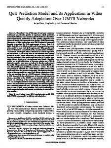
The remarkable point on the Pareto-Box problem is that it establishes the fact that the probability of finding dominated points in higher dimensions (i.e. increasing number of objectives) is falling exponentially with the dimension of the problem. Having a look on most prominent EMO algorithms like NSGA-II [5], SPEA2 [4] or PESA [10], it can be seen that they all need dominated points to perform their processing steps. For still yielding dominated points in the domain of higher number of objectives, these algorithms need an exponetially increasing search effort, be it by increasing the population size, or be it by increasing the number of generations. The advantage of the FPD is that the problem of missing dominated points does not matter. This will be demonstrated by using the Pareto-Box problem. Figure 3 compares the performance of comparable set-ups of NSGA-II and FDD-GA on the Pareto-Box problem for dimension n = 20. The NSGA-II implementation strictly followed [4]. For both algorithms, the population size was 10, and 200 generations were performed. Both algorithm used the same mutation probability and strength of 0.1. The selection scheme of FDD-GA was adapted due to having a known co-domain of the ranking values (aka fitness values). Roulette-wheel selection was performed using − ln ri (with ri the ranking values) as shared fitness values, and it was only selected among the non-dominated individuals. If all individuals got the same ranking values, it was randomly selected. The plot shows the size of the archive over the number of sample points (i.e. calls of the objective functions). Also given is the (numerically estimated) size of the Pareto-set for random sampling, and the total number of individuals (dominated and non-dominated). As established by Theorem 3, for random search the size of the Pareto set is close to the total number of points. However, also NSGA-II runs close to this curve, qualifying this search as more or less random as well. This is obvious from the fact that the probability of finding a dominated individual by applying randomized operators (mutation, crossover)
Archive Sizes 2000
All Random FPDGA NSGA-II
1800
1600
Size of Pareto set
1400
1200
1000
800
600
400
200
0 0
100
200
300
400
500
600
700
800
900
1000 1100 1200 1300 1400 1500 1600 1700 1800 1900 2000
Number of sample points
Fig. 3. Performances of NSGA-II and FDD-GA for the Pareto-Box problem.
is low. The performance will increase when using a larger population, however, the results from the foregoing section give that the population size has to be increased exponentially, in order to achieve such a goal. For FDD-GA, we clearly see that even for dimension 20, and a rather small population size of 10 individuals, it is able to find the single optimum of the Pareto-Box problem, and also stays strongly below the curve of random search all the time. To make this behaviour more clear, we considered the p.d.f. of the ranking values within a randomly created population (see fig. 4). This plot was obtained by 100 times creating a set of 20 random vector with 100 components from [0, 1]. Then, among these 20 vectors the ranking values ri were computed, and the intervall frequencies for − ln ri were derived. Thus, we can model the handling of randomly selected points by the FPD ranking scheme (as it happens when applied to the Pareto-Box problem). The distribution has a tail at the sider of smaller ranking values, so roulette-wheel selection will acknowledge the fact that such individuals gradually perform better (with respect to Paretodominance). Such a behaviour can not be achieved when an EMO is relying on the presence of dominated individuals alone. It has to be noted (but will not be detailed here) that nevertheless NSGA-II, in this set-up, is also finding the optimum up to a problem dimension of 8. In low dimensions (2-3) the FDD-GA is also outperformed by NSGA-II.
120
100
h
80
60
40
20
67
64
62
60
58
56
54
52
50
48
46
44
42
40
38
36
34
32
30
28
26
24
0 -ln r
Fig. 4. Distribution of ranking values in FDD-GA algorithm.
6
Conclusions
In this paper, issues related to the fuzzification of Pareto dominance were considered. A ranking scheme was presented that assigns dominance degrees to any set of vectors in a scale-independent, non-symmetric and set-dependent manner. Based on such a ranking scheme, the vector fitness values of a population can be replaced by the computed ranking values (representing the ”dominating strength” of an individual against all other individuals in the population) and used to perform standard single-objective genetic operators. The corresponding extension of the Standard Genetic Algorithm, the FDD-GA, was presented as well. To verify the usefulness of such an approach, an analytic study of the Pareto-Box problem was provided, showing the characteristical parameters of a random search for the Pareto front in a unit hypercube in arbitrary dimension. The basic problem here is the loss of dominated points with increasing problem dimension, which can be successfully resolved by founding the search procedure on the fuzzy dominance degrees.
Acknowledgment The research presented in this paper was supported by German research project ”VisionIC,” funded by German Ministry of Research and Education (BMBF) as
handled by ”Deutsche Gesellschaft f¨ ur Luft- und Raumfahrt” (DLR). The authors also would like to express their thanks to Frank Hoffmann from University of Dortmund and Anna Ukovich from University of Trieste for their valuable comments and inspiring discussions about the topics of this work.
References 1. Coello Coello, C.A.: A short tutorial on evolutionary multiobjective optimization. In Zitzler, E., Deb, K., Thiele, L., Coello, C.A.C., Corne, D., eds.: First International Conference on Evolutionary Multi-Criterion Optimization. Volume 1993 of Lecture Notes in Computer Science. Springer Verlag (2001) 21–40 2. Coello Coello, C.A.: An updated survey of GA-based multiobjective optimization techniques. Technical Report RD-98-08, Laboratorio Nacional de Inform´ atica Avanzada (LANIA), Xalapa, Veracruz, M´exico (1998) 3. Fonseca, C.M., Fleming, P.J.: An overview of evolutionary algorithms in multiobjective optimization. Evolutionary Computation 3(1) (1995) 1–16 4. Deb, K., Agrawal, S., Pratap, A., Meyarivan, T.: A fast elitist non-dominated sorting genetic algorithm for multi-objective optimization: NSGA-II. In Schoenauer, M., Deb, K., Rudolph, G., Yao, X., Lutton, E., Merelo, J.J., Schwefel, H.P., eds.: Proceedings of the Parallel Problem Solving from Nature VI Conference. Volume 1917 of Lecture Notes in Computer Science., Paris, France, Springer (2000) 849–858 5. Zitzler, E., Laumanns, M., Thiele, L.: SPEA2: Improving the strength pareto evolutionary algorithm. Technical Report 103, Computer Engineering and Networks Laboratory (TIK), Swiss Federal Institute of Technology, Zurich, ETH Zentrum, Gloriastr 35, CH-8092 Zurich, Switzerland (2001) 6. Farina, M., Amato, P.: Fuzzy optimality and evolutionary multiobjective optimization. In C.M. Fonseca et al., ed.: EMO 2003, LNCS 2632. (2003) 58–72 7. K¨ oppen, M., Franke, K., Nickolay, B.: Fuzzy-pareto-dominance driven multiobjective genetic algorithm. In: Proceedings of the 10th IFSA World Congress. (2003) 450–453 8. Okabe, T., Jin, Y., Sendhoff, B.: A critical survey of performance indices for multiobjective optimization. In: Proceedings of the 2003 Congress on Evolutionary Computation (CEC’2003), Canberra, Australia, IEEE Press (2003) 878–885 9. K¨ oppen, M., Vicente Garcia, R.: A fuzzy scheme for the ranking of multivariate data and its application. In: Proceedings of the 2004 Annual Meeting of the NAFIPS (CD-ROM), Banff, Alberta, Canada, NAFIPS (2004) 140–145 10. Corne, D.W., Knowles, J.D., Oates, M.J.: The pareto envelope-based selection algorithm for multiobjective optimization. In: Proceedings of the Parallel Problem Solving from Nature VI Conference. Volume 1917 of Lecture Notes in Computer Science., Springer (2000) 839–848
Appendix Derivation of Theorems 1 and 2 Here, we shortly sketch the derivation of Theorems 1 and 2. For general dimensions n we assign ranking vectors to all m point. We indicate the coordinate
directions with x1 , x2 , . . . , xn . If a point Pi gets assigned the ranking vector (i1 , i2 , . . . , in ) with ik ∈ {1, 2, . . . , m} this means that the x1 coordinate of this point is the i1 -th smallest among all the m x1 -coordinates of the m points, the x2 -coordinate is the i2 -th smallest among all x2 -coordinates of the m points and so forth. For all m points and all 1 ≤ k ≤ n, the ranking vectors at position k form a permutation of the set {1, 2, . . . , m}. So, a set of n permutations of the set {1, 2, . . . , m} may be derived from any selection of m points. However, a ranking scheme is already sorted into one dimension, e.g. the x1 -dimension, so only (n−1) permutations are independent. As a result, there are m!n−1 different ranking schemes for m points in n dimensions. Among the m points there is one point Pl with the largest x1 -coordinate value. We consider the projection of all m points into the (n − 1)-dimensional ranking scheme, spanned by the coordinates x2 , x3 , . . . , xn and x1 = n. There are m!n−2 such ranking schemes, and each of them will be obtained by the projection of m! different n-dimensional ranking schemes (since m!n−1 /m!m−2 = m!).
Fig. 5. Entering the three points (0.1, 0.3, 0.6), (0.3, 0.4, 0.1) and (0.5, 0.5, 0.3) into one of the 3!2 = 36 ranking schemes for 3 points in 3 dimensions, together with the projections into 2-dimensional ranking schemes of 3 points. Two of the projections specify the ranking scheme completely, since the points are already sorted in the third dimension. The analysis is based on the fact that the Pareto set size of this ranking scheme is the Pareto set size of the two points with the lowest x-coordinate plus 1 in case the point with the largest x-coordinate is projected onto a point of the Pareto set of the projected ranking scheme, which is parallel to the (y, z)-plane.
Now, a moment of reasoning gives that the point Pl will belong to the Pareto set of the n-dimensional ranking scheme if and only if its projection belongs to
the Pareto set of the (n − 1)-dimensional projected ranking scheme: We are considering whether the point P , onto which Pl is projected, belongs to the Pareto set of the (n − 1)-dimensional projected ranking scheme or not. If it belongs to the Pareto set of the (n−1)-dimensional ranking scheme, this means that there is no other point having lower ranking positions than P in all the dimensions x2 , x3 , . . . , xn simultaneously. But this means that there is also no point in the n-dimensional ranking scheme having lower ranking positions than Pl in all the dimensions x1 , x2 , x3 , . . . , xn simultaneously as well. Thus, if Pl is projected onto an element of the Pareto set of the (n − 1)-dimensional ranking scheme, it belongs to the Pareto set of the n-dimensional ranking scheme. If P does not belong to the Pareto set of the (n − 1)-dimensional projected ranking scheme, there is another point P1 in the projected (n − 1)dimensional ranking scheme having lower ranking positions than P in all dimensions x2 , x3 , . . . , xn simultaneously. Once Pl is projected onto this point, it has to be taken into account that Pl is the point with the highest x1 -coordinate value, so each other point in the n-dimensional ranking scheme will have a lower x1 -coordinate value, including the point from which P1 originated. So, there is a point in the n-dimensional ranking scheme dominating Pl and Pl will not belong to the Pareto set of the n-dimensional ranking scheme. The Pareto set of the (m − 1) points different from Pl is not influenced by Pl , since Pl can never dominate any of these points (it fails already to dominate in the x1 -coordinate). So, the size of the Pareto set of the m points is either Ps or Ps + 1, with Ps being the size of the Pareto set of the (m − 1) points that are different from Pl . It is Ps + 1 if Pl belongs to the Pareto set of the ndimensional ranking scheme, Ps otherwise. But we have just seen that Pl belongs to the Pareto set of the n-dimensional ranking scheme if and only if it belongs to the Pareto set of the (n − 1)-dimensional projected ranking scheme. Putting it all together: – There are m!n−1 different ranking schemes for m points in the n-dimensional hypercube. We denote them by R1 , R2 , . . . , RN . – Each of these ranking schemes Ri can be related to a ranking scheme Sj of (m − 1) points in n dimensions by removing the point Pl with the largest x1 coordinate (j = 1, . . . , (m−1)!n−1 ). Given any ranking scheme Sj for (m−1) points in the n-dimensional hypercube, it can be made a ranking scheme of m points in n dimensions by adding a ”last” point Pl to it. The number of ways to add the m-th point to a ranking scheme Sj does not depend on the ranking scheme itself, so any Sj can generate the same number of Ri , say l. It follows l = m!n−1 /(m − 1)!n−1 = mn−1 . – Each Ri can be projected into a ranking scheme si of m points in the (n − 1)-dimensional hypercube by removing the ranking according to the x1 -coordinate (i = 1, . . . , m!n−2 ). There are always m! ranking schemes Ri that are projected into the same sj . – The size of the Pareto set of a ranking scheme Ri will be denoted by ri , the size of the Pareto set of a ranking scheme Si by pi and the size of the Pareto set of a ranking scheme si by qi .
– From the m! cases that a ranking scheme Ri is projected onto a ranking scheme sj with Pareto set size qj , in exactly m! · qj /m = (m − 1)! · qj cases its point Pl with the largest x1 -coordinate will be projected into an element of the Pareto set of sj , thus belong to the Pareto set of Ri in addition to the ri points that comprise the Pareto set of the (m − 1) points different from Pl . Now we sum the Pareto set sizes over all Ri and divide by the number of Ri to get the expectation value em (n). We can decompose this sum into two contributions: the contributions coming from the reduced ranking schemes Si with Pareto set sizes pi and the contribution coming from the Pareto sets of the projected ranking schemes si with Pareto set sizes qi : n−1
m! X 1 em (n) = rk n−1 m! k=1 n−2 (m−1)!n−1 m! X X 1 n−1 = m pk + (m − 1)! qk m!n−1 k=1
(8)
k=1
� 1 � n−1 m · em−1 (n) · (m − 1)!n−1 + (m − 1)! · em (n − 1) · m!n−2 m!n−1 1 = em−1 (n) + em (n − 1) m =
by using that the sum of all pi equals the expectation value for (m − 1) points in the n-dimensional hypercube times the number (m − 1)!n−1 of their ranking schemes Si , and the sum of all qi equals the expectation value for m points in (n − 1) dimensions times the number m!n−2 of their ranking schemes si . When adding the obvious relations e1 (n) = em (1) = 1 this will give Theorem 1. By showing that the expression in eq. (6) fulfills the recursive equation in Theorem 1, Theorem 2 can be established as well. The proof goes via complete induction over n and m.