Astronomy & Astrophysics
A&A 616, A5 (2018) https://doi.org/10.1051/0004-6361/201832763 © ESO 2018
Special issue
Gaia Data Release 2
Gaia Data Release 2 Gaia Radial Velocity Spectrometer M. Cropper1 , D. Katz2 , P. Sartoretti2 , T. Prusti3 , J. H. J. de Bruijne3 , F. Chassat4 , P. Charvet4 , J. Boyadjian4 , M. Perryman5 , G. Sarri3 , P. Gare3 , M. Erdmann3 , U. Munari6 , T. Zwitter7 , M. Wilkinson8 , F. Arenou2 , A. Vallenari9 , A. Gómez2 , P. Panuzzo2 , G. Seabroke1 , C. Allende Prieto1,10 , K. Benson1 , O. Marchal2 , H. Huckle1 , M. Smith1 , C. Dolding1 , K. Janßen11 , Y. Viala2 , R. Blomme12 , S. Baker1 , S. Boudreault1,13 , F. Crifo2 , C. Soubiran14 , Y. Frémat12 , G. Jasniewicz15 , A. Guerrier16 , L. P. Guy17 , C. Turon2 , A. Jean-Antoine-Piccolo18 , F. Thévenin19 , M. David20 , E. Gosset21,22 , and Y. Damerdji21,23 1 2 3 4 5 6 7 8 9 10 11 12 13 14 15 16 17 18 19 20 21 22 23
Mullard Space Science Laboratory, University College London, Holmbury St Mary, Dorking, Surrey RH5 6NT, UK e-mail:
[email protected] GEPI, Observatoire de Paris, Université PSL, CNRS, 5 Place Jules Janssen, 92190 Meudon, France ESA, European Space Research and Technology Centre (ESTEC), Keplerlaan 1, 2201 AG Noordwijk, The Netherlands Airbus Defence and Space, 31 Rue des Cosmonautes, 31402 Toulouse Cedex, France Scientific Support Office, Directorate of Science, European Space Research and Technology Centre (ESA/ESTEC), Keplerlaan 1, 2201 AZ, Noordwijk, The Netherlands INAF – National Institute of Astrophysics, Osservatorio Astronomico di Padova, Osservatorio Astronomico 6, 36012 Asiago, Italy Faculty of Mathematics and Physics, University of Ljubljana, Jadranska ulica 19, 1000 Ljubljana, Slovenia Department of Physics & Astronomy, University of Leicester, University Road, Leicester LE1 7RH, UK INAF - Padova Observatory, Vicolo dell’Osservatorio 5, 35122 Padova, Italy Instituto de Astrofísica de Canarias, 38205 La Laguna, Tenerife, Islas Canarias, Spain Leibniz Institute for Astrophysics Potsdam (AIP), An der Sternwarte 16, 14482 Potsdam, Germany Royal Observatory of Belgium, Ringlaan 3, 1180 Brussels, Belgium Max Planck Institut für Sonnensystemforschung, Justus-von-Liebig-Weg 3, 37077 Göttingen, Germany Laboratoire d’Astrophysique de Bordeaux, Université de Bordeaux, CNRS, B18N, Allée Geoffroy Saint-Hilaire, 33615 Pessac, France Laboratoire Univers et Particules de Montpellier, Université Montpellier, Place Eugène Bataillon, CC72, 34095 Montpellier Cedex 05, France Thales Services, 290 Allée du Lac, 31670 Labège, France Department of Astronomy, University of Geneva, Chemin d’Ecogia 16, 1290 Versoix, Switzerland Centre National d’Études Spatiales, 18 Avenue Edouard Belin, 31400 Toulouse, France Laboratoire Lagrange, Université Nice Sophia-Antipolis, Observatoire de la Côte d’Azur, CNRS, CS 34229, 06304 Nice Cedex, France Universiteit Antwerpen, Onderzoeksgroep Toegepaste Wiskunde, Middelheimlaan 1, 2020 Antwerpen, Belgium Institut d’Astrophysique et de Géophysique, Université de Liège, 19c, Allée du 6 Août, 4000 Liège, Belgium F.R.S.-FNRS, Rue d’Egmont 5, 1000 Brussels, Belgium CRAAG - Centre de Recherche en Astronomie, Astrophysique et Géophysique, Route de l’Observatoire, Bp 63 Bouzareah, 16340 Algiers, Algeria
Received 3 February 2018 / Accepted 21 February 2018 ABSTRACT
This paper presents the specification, design, and development of the Radial Velocity Spectrometer (RVS) on the European Space Agency’s Gaia mission. Starting with the rationale for the full six dimensions of phase space in the dynamical modelling of the Galaxy, the scientific goals and derived top-level instrument requirements are discussed, leading to a brief description of the initial concepts for the instrument. The main part of the paper is a description of the flight RVS, considering the optical design, the focal plane, the detection and acquisition chain, and the as-built performance drivers and critical technical areas. After presenting the pre-launch performance predictions, the paper concludes with the post-launch developments and mitigation strategies, together with a summary of the in-flight performance at the end of commissioning. Key words. space vehicles: instruments – instrumentation: spectrographs – surveys – techniques: spectroscopic – techniques: radial velocities
1. Introduction The Gaia satellite of the European Space Agency (ESA) was launched on 2013 December 19, arriving at the L2 point a month
later, for a planned five-year mission after the commissioning, which ended in 2014 July (the mission was extended for a further 1.5 years in late 2017). Gaia was conceived as an astrometric satellite, extending by orders of magnitude in terms
Article published by EDP Sciences
A5, page 1 of 19
A&A 616, A5 (2018)
of distance and accuracy the pioneering results from ESA’s H IPPARCOS satellite. The mission, a collaboration between ESA, industrial partners, and science institutes in ESA member states, is described in Gaia Collaboration (2016b). The first data release was made in 2016 September and is described in Gaia Collaboration (2016a). The science return from H IPPARCOS is very significant (see Perryman (2009) for a comprehensive overview), but its payload permitted only astrometric and photometric measurements. Measurement of stellar positions over time produced proper (transverse) motions and distances, but not a measure of the velocity in the line of sight (the radial velocity). This was recognised as a deficiency at the time; see for example Blaauw in Torra et al. (1988). Perryman (2009) provides a comprehensive overview of the proposals made in France and the UK and also within ESA in the period 1980–1987 for new dedicated telescopes and updated instrumentation. None of these was successful. Emphasising that for many studies it is of the greatest importance to have all three space velocities rather than only the two components of the star’s velocity on the sky, Binney et al. (1997) noted how few stars in the H IPPARCOS Input Catalog (Turon et al. 1992) had radial velocities. A ground-based ESO Large Programme was instigated to provide radial velocities of the ∼60 000 stars in the H IPPARCOS Input Catalog with spectral type later than F5, but progress was slow. The situation improved only when Nordström et al. (2004) published good measurements for ∼13 500 F and G dwarfs and Famaey et al. (2005) published radial velocities for 5952 K and 739 M giants, but this was still a small fraction of the total catalogue1 . This shortcoming was therefore fully evident at the time when the early Gaia concepts were being developed, and hence a spectrometer, the Radial Velocity Spectrometer (RVS), was incorporated into the payload to avoid such a science loss (Favata & Perryman 1995, 1997). Beyond the radial velocities, this initiative also for the first time enabled a spectroscopic survey of the entire sky to measure astrophysical parameters of point sources. Perryman (1995) emphasised the scientific utility from acquisition of information complementary to the astrometric measurements in the Gaia (Lindegren & Perryman 1996) and Roemer (Høg & Lindegren 1994) concepts being developed at that time. In addition to providing full space motions, he identified the advantages to the mission of multiple visits for identifying binary systems, and correction of perspective accelerations, and also the wider benefits of the large-scale determination of elemental chemical abundances that would inform the star formation history and provide chemical enrichment information, to parallel that from the kinematic measurements. The paper highlighted the scale of the task, given the significant increase in kinematic data in the mission concepts. While Perryman (1995) mainly considered ground-based solutions using multi-fibre spectrographs, it was clear that a dedicated instrument in orbit would provide more complete and uniform complementary information. The initial concept presented in Favata & Perryman (1995, 1997) was a slitless scanning spectrograph called the Absolute Radial Velocities Instrument (ARVI). This would provide a radial velocity precision of ∼10 km s−1 at a limiting magnitude of ∼17, with ∼1 km s−1 for brighter magnitudes 10–12, to achieve a metallicity determination precision of ∼0.1 dex. The instrument would use a separate 1
Since that time, several large spectroscopic surveys for galactic science have been undertaken, including RAVE (Steinmetz et al. 2006), APOGEE (Majewski et al. 2017), ESO-Gaia (Gilmore et al. 2012), LAMOST (Cui et al. 2012), and GALAH (Martell et al. 2017). A5, page 2 of 19
optical system to that for the astrometry. Many of the critical aspects important in the long-term for the RVS were discussed in the ARVI papers, including the limiting magnitude, resolution, bandpass, scanning rate, telemetry- and attitude-control requirements, and the wavelength zero point. Taken together with the photometric measurements planned in the Gaia mission concept (to provide luminosities and temperatures, as well as photometric distances and ages), the change in emphasis for this next generation of mission should not be underestimated. Through the acquisition of both kinematic and astrophysical data, Gaia was developed from an advanced astrometric satellite into a complete facility for the study of the formation and evolution of the Galaxy. This paper provides a brief overview of the RVS concept and requirements (Sects. 3 and 4) and then describes the instrument (Sects. 5–7) before examining the pre-launch performance (Sect. 8). Post-launch developments, optimisations, and updated performance predictions are summarised in Sects. 9–11. We distinguish in this paper between pre-launch instrument parameters – for example as implemented at the critical design review (CDR) or derived from the ground-based calibrations – and those post-launch, after which they may have been optimised for the in-orbit characteristics of the satellite during commissioning. It should be kept in mind that the in-orbit performance described from Sect. 9 onwards supersedes the pre-launch expectations, and also that the full end-to-end performance of the RVS instrument is achieved in conjunction with the full Gaia dataprocessing system, described in Sartoretti et al. (2018) and Katz et al. (2018).
2. Early RVS concepts Subsequent to Gaia’s adoption in 2000 October initiating the major industrial activities, ESA in mid-2001 instigated working groups for the scientific community to contribute to the development of the mission. One of these was the RVS Working Group. In the period 2001–2006, this group examined in detail the scientific requirements of the instrument. Fundamental considerations included the wavelength range of the spectrometer, spectral resolution, and the limiting magnitude. Because Gaia would operate in time-delay integration (TDI) mode, in which the spectra would scan over the focal plane at the same rate at which the CCD detectors were being read out, RVS would necessarily be slitless. To minimise the background light, the wavelength range should be as narrow as possible, consistent with it containing sufficient strong spectral lines to provide radial velocity information, as well as an adequate range of chemical elements to provide astrophysical information (temperatures, gravities, and metallicities). Spectral regions around the Mg II doublet at ∼440 nm and the Ca II triplet at ∼850 nm were examined, with a 25 nm region centred on the Ca II triplet preferred (this spectral domain was originally proposed by U. Munari, and noted independently by R. Le Poole). The balance between the radial velocity and astrophysical information (requiring higher signal-to-noise ratios - S/Ns) for the setting of the resolving power requirements between R = 5000 and 20 000 was explored, with R = 11 500 found to be optimal in providing both adequate spectral resolution while maximising the radial velocity performance, and taking into account other factors as well, such as the telemetry budget. Because the RVS bandpass is narrow compared to that of the astrometric instrument, so that fewer photons are recorded,
M. Cropper et al.: Gaia Data Release 2
and because the spectral dispersion distributes these over a larger number of pixels, each of which has associated noise sources, the limiting magnitude would necessarily be lower. It was therefore important to consider the scientific drivers carefully and match the radial velocity accuracy with that of the transverse velocities for the scientific scenarios of interest. These considerations set requirements of 3–15 km s−1 for V = 16.5 K-type giants (Wilkinson et al. 2005). These and other requirements were consolidated for the spectroscopic requirements in the Mission Requirements Document for the Implementation Phase of the programme (Gaia Project Team 2005). At the start of the implementation phase, the working groups were shut down and the expertise was transferred to the Gaia Data Processing and Analysis Consortium (DPAC). Over the same period, ESA and some European agencies funded an engineering study led by a consortium constituted from science institutes, with the aim of complementing the work of the industrial teams, who were concentrating mainly on the astrometric performance of Gaia during this competitive tendering phase. Based on the earlier Phase A activities, the payload concept at that point contained a separate telescope (Spectro) for the RVS and medium-band photometry (see for example MMS Study Team 1999; Merat et al. 1999; Perryman et al. 2001; Safa et al. 2004). In this complementing study by the RVS Consortium, the driving performance considerations for the instrument design were to maximise the radial velocity precision, and to minimise the constraints imposed by the telemetry limitations. The signal levels were increased by maximising the field of view and reducing the focal ratio consistent with optical distortion and spectral resolution, in order to reduce the scanning speed over the detector and maximise the exposure duration. The principal noise source was identified as that arising in the detector from the readout (readout noise), so electron-multiplying CCDs (also known as L3CCDs) were specified to reduce this to a minimum. Although a generous fraction of the overall Gaia telemetry was allocated to the RVS, the length of the spectra imposed high data rates, and this, with the desirability of two-dimensional information to separate overlapping spectra optimally, led to a scheme in which data from the CCDs were combined on board in order to remain within the budget. Performance predictions and system margins were within budget. The work during this period was reported in Katz (2003, 2005); Katz et al. (2004), Munari et al. (2003), Cropper (2003), Cropper et al. (2005a,b), and especially in Katz et al. (2004) and Wilkinson et al. (2005). For the implementation phase in 2006, the selected prime contractor Astrium (now Airbus Defence and Space) proposed and implemented a different RVS instrument concept, in part using ideas in Cropper & Mason (2001).
3. Flight instrument concept The flight RVS design departed from the earlier concepts discussed briefly in Sect. 2 above by removing the Spectro telescope, and employing, instead, the telescopes for the astrometric instrument. This was motivated by savings in mass, power (and heat dissipation), improved payload module accommodation, and cost. The starlight is dispersed by a block of RVS optics, which produces a spectrum that is approximately confocal with the undispersed beams, and with the same focal ratio. The optics block also defines the instrument bandpass and corrects the off-axis characteristics of the beam. The RVS focal
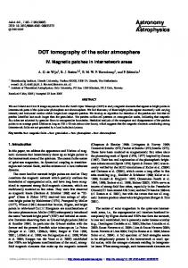
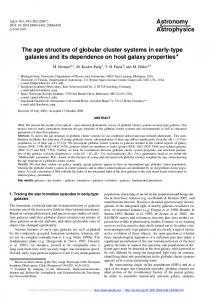
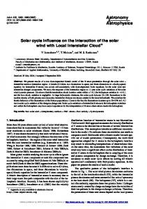
Fig. 1. Layout of the optical beams after the beam combiner from the two telescopes, and the focal plane in Gaia. The scan direction is from right to left. BAM is the Basic Angle Monitor, and WFS is the Wavefront Sensor.
plane is located in the same focal plane array as the astrometric instrument. Starlight enters the spectrometer after the astrometric (and photometric) instruments during normal operations when the satellite is scanning. There are 12 CCDs in the RVS focal plane. In order to limit the size of the elements in the optics block, only four rows of CCDs are employed, instead of seven in the astrometric focal plane. The instrument uses the SkyMapper information from the astrometric field of view. The median optical spectral resolving power of 10 400 was compliant with the nominal requirement (Gaia Project Team 2005), and with a sampling of ∼3 pixels per resolution element, the window was 1260 pixels long. This layout is shown schematically in Fig. 1. The RVS is considered to consist of the RVS optics block, the focal plane, and the dedicated software to place windows on the focal plane. The instrument and its operation with other payload elements including the SkyMappers is described briefly in Gaia Collaboration (2016b). The flight design therefore benefits from the larger light grasp of the telescopes feeding the astrometric instrument, and with two telescopes, the doubling of the number of observations of each object, as well as from the removal of an entire optical system with its separate star trackers. However, the integration time per CCD is limited to the same as that of the astrometric instrument, 4.4 s, which significantly reduces the exposure levels with respect to the earlier concept (in which the focal ratio was shorter and the field of view larger), and the smaller number of rows of CCDs in the RVS focal plane reduces the number of observations per object. With respect to the performance expected in the earlier concepts discussed in Katz et al. (2004), and from a different perspective, in Cropper et al. (2004, 2005a), the projected pre-launch limiting magnitude of the flight design was ∼1 magnitude poorer owing to the shorter exposure times from the telescopes, and conventional CCDs, rather than L3CCDs in the focal plane, with implications for the science case discussed in Wilkinson et al. (2005). On the other hand, with the experience of processing in-orbit RVS data, the longer focal length arising from the use of the same telescope as that for the astrometric instrument significantly reduces the spectral overlapping, enhancing the performance when one or both telescopes scan crowded regions of the sky. A5, page 3 of 19
A&A 616, A5 (2018) Table 1. Top-level RVS-specific requirements.
Average number of transits over mission Wavelength range Spectral resolving power (HR mode) Spatial resolution Maximum stellar density Maximum apparent brightness Minimum apparent brightness Radial velocity systematic error after calibration Radial velocity precision of 1 km s−1 Radial velocity precision of 15 km s−1
40 for objects V < 15 847–874 nm average 10 500–12 500; 90% ≥10 000; max 13 500 1.8 arcsec to include 90% of flux 36 000 objects degree−2 all spectral types V 13 G2V V > 17 K1IIIMP V > 19 ≤300 m s−1 at end of mission B1V V ≤7 G2V V ≤ 13 K1III MP V ≤ 13.5 B1V V ≤ 12 G2V V ≤ 16.5 K1III MP V ≤ 17
Notes. Additional requirements include the capability for operation in HR and LR mode (see text), at least Nyquist spectral sampling for HR mode, control over flux rejection levels outside the RVS bandpass, and straylight requirements applicable to the payload as a whole. Spectral types follow the standard terminology, so that temperature decreases from B to K stars, V in the spectral identifier denotes dwarfs, and IIIMP denotes metal poor giants. From Colangelo (2010).
4. Requirements Before describing the instrument in more detail, we identify in Table 1 the RVS-specific top level requirements guiding its design. These are extracted from the ESA Mission Requirements Document (Colangelo 2010), revised to take into account the developments in Sect. 3 and hence applicable to the asimplemented instrument. The methodology to be applied to the radial velocity predictions was specified in de Bruijne et al. (2005a). The context for some of these requirements is elaborated in the following subsections. Because of higher scattered light levels encountered in orbit (Sect. 9), some of the considerations discussed below required reassessment during the commissioning phase, as described in Sects. 10 and 11. 4.1. Limiting magnitude and wavelength range
The RVS is an atypical spectrometer in that it is slitless while providing medium resolving power, with constrained exposure durations. Consequently, at intermediate and faint magnitudes, it is photon starved and noise dominated. For its role in providing radial velocities, information from the entire spectrum is condensed into a single velocity value through a cross-correlation, with the radial velocity signature at the faint end emerging only after adding many transits of the object during the survey. Even at the end of the mission, the spectra of most stars will be noise dominated, and will produce only a radial velocity. Simulations (Katz et al. 2004) showed that final S/N of ∼1 per spectral resolution element would nevertheless provide sufficient end-of-mission radial velocity precision. Hence, regardless of the instrument design, at its limiting magnitude and after the noise was minimised, the RVS measurements would have on average 10 in which pixels could be summed at the detector readout node to reduce the readout noise per sample. The requirements on the detector readout noise as derived from the limiting magnitude performance was set at ≤4.0 e− for LR mode and ≤6.0 e− for HR. Gaia is required to scan the sky as uniformly as possible, and to measure the angular distances between stars in the astrometric fields of view at a range of orientations. The adopted scanning law is one of forced precession (Gaia Collaboration 2016b), which results in a sideways (across-scan, AC) displacement (with a sinusoidal dependence) of the star on the spin period of the satellite. In order to maintain the spectral resolving power, the orientation of the dispersion direction was set along the scanning direction (AL) so that spectral lines were not broadened by this AC displacement (Cropper & Mason 2001; Katz et al. 2004). The (lesser) consequence was that the spectra were broadened with a spatial distribution at a period half that of the spin period, leading to a variation in S/N on the same period. 4.3. Radiation damage
As noted in Sect. 4.1 above, at its limiting magnitude, the RVS instrument concept will work with