Sep 22, 2004 - the loop fusion problem considering both timing and code ..... retiming values computed by the Bellman-Ford algorithm are r(a) = (0, 3), r(b) = (0 ...
General Loop Fusion Technique for Nested Loops ∗ Considering Timing and Code Size Meilin Liu,
Qingfeng Zhuge, Zili Shao, Edwin H.-M. Sha Department of Computer Science University of Texas at Dallas Richardson, Texas 75083, USA {mxl024100, qfzhuge, zxs015000, edsha}@utdallas.edu
ABSTRACT
1. INTRODUCTION
Loop fusion is commonly used to improve the instructionlevel parallelism of loops for high-performance embedded computing systems. Loop fusion, however, is not always directly applicable because the fusion prevention dependencies may exist among loops. Most of the existing techniques still have limitations in fully exploiting the advantages of loop fusion. In this paper, we present a general loop fusion technique for loops or nested loops based on the loop dependency graph model, retiming, and multi-dimensional retiming concepts. We show that any “J+K” model loop can be legally fused using our legalizing fusion technique. Polynomial-time algorithms are developed to solve the loop fusion problem for “J+K” model loops considering both timing and code size of the final code. Our technique produces the final code and calculates the resultant code size directly from the retiming values. The experimental results show that our loop fusion technique always significantly reduces the schedule length.
Embedded systems usually have strict timing requirement. Many embedded systems are equipped with multiple functional units or processors, such as VLIW or system-on-achip, to satisfy the ever-growing performance requirements. Much of the computation involved in embedded system occurs within loops. Loop transformations such as loop alignment, loop skewing and loop tiling can be used to optimize the execution of the loops[5, 13, 20, 1, 3, 10]. Loop fusion is to combine and transform multiple loops into one loop and it is commonly used to improve the instruction-level parallelism in the embedded system with multiple functional units[16]. Loop fusion can also be used to enhance data locality so that memory references and power consumption can be reduced[9, 6, 11, 18, 2, 19]. But loop fusion is not always applicable because of the existence of conflict data dependencies among loops. Most of the existing techniques still have limitations in exploring the potential opportunities of loop fusion [7, 6, 16, 11, 18, 2]. Many loop fusion techniques try to solve problems by directly dealing with compiled code and loop index computation, which is lack of an effective analysis model and inefficient for embedded system design. Furthermore, the existing loop fusion techniques do not consider the resultant code size of a fused loop which is another critical concern for the design of embedded systems [21, 4]. Therefore, a systematic approach to solve the loop fusion problem considering both timing and code size is necessary for fully exploiting the advantages of loop fusion and avoiding ad-hoc practices. In this paper, we propose a general loop fusion technique to maximize the opportunities of loop fusion for nested loops. The loop fusion problem for simple loops becomes a special case of the application of our technique. In the following, we show an example of loop fusion problem. The code shown in Figure 1(a) contains three sequential loops enclosed in a shared outermost loop. But these loops cannot be directly fused because of the conflict data dependencies existing among them. First, we found that the loops a and b cannot be combined into one loop because we need the value of A[i][j + 1] to compute B[i][j]. Obviously, the value A[i][j + 1] is not available in the (i, j)th iteration. This kind of dependency is called fusion-prevention dependency which can be represented by a negative weight edge in a loop dependency graph (LDG) with nodes representing loops as shown in Figure 2(a). We use the graph representation of loops in this paper and will give a detailed explanation later. Second, we found another fusion-prevention dependency be-
Categories and Subject Descriptors C.3 [Computer Systems Organization]: Special-Purpose and Application-Based Systems—real-time and embedded systems, signal processing systems;
General Terms Algorithms, Performance, Experimentation
Keywords Loop Fusion, Retiming, Scheduling, Code size, Embedded DSP ∗This work is partially supported by TI University Program, NSF EIA-0103709, Texas ARP 009741-0028-2001 and NSF CCR-0309461, USA.
Permission to make digital or hard copies of all or part of this work for personal or classroom use is granted without fee provided that copies are not made or distributed for profit or commercial advantage and that copies bear this notice and the full citation on the first page. To copy otherwise, to republish, to post on servers or to redistribute to lists, requires prior specific permission and/or a fee. CASES’04, September 22–25, 2004, Washington, DC, USA. Copyright 2004 ACM 1-58113-890-3/04/0009 ...$5.00.
for i=0, N for j=0,M A[i,j]=C[i−2,j+1]; endfor for j=0, M B[i,j]=A[i,j+1]+A[i,j]+C[i−1,j]; endfor for j=0, M C[i,j]=B[i,j]+A[i,j+2]+A[i,j+1]; endfor endfor
a
r(a)=(0,2)
a
(a) (0,0)
(0,−1)
(b) b
(c)
(1,0)
(0,−2)
(2,−1)
r(b)=(0,1)
(0,0)
(1,−1)
r(c)=(0,0)
c
b
(0,0)
(2,−3)
(0,1)
c
(a) (a) for i=0, N A[i,0]=C[i−2,1]; A[i,1]=C[i−2,2]; B[i,0]=A[i,0]+A[i,1]+C[i−1,0];
(b)
Figure 2: (a)The LDG of the loop shown in Figure 1(a). Prologue
(b)The retimed LDG with retiming ~r(a) = (0, 2), ~ r (b) = (0, 1), and ~r(c) = (0, 0).
for j=0, M A[i,j+2]=C[i−2,j+3]; B[i,j+1]=A[i,j+2]+A[i,j+1]+C[i−1,j+1]; C[i,j]=B[i,j]+A[i,j+1]+A[i,j+2];
Fused Loop Body
endfor B[i,M]=A[i,M]+A[i,M+1]+C[i−1,M]; C[i,M−1]=B[i,M−1]+A[i,M]+A[i,M+1]; C[i,M]=B[i,M]+A[i,M=1]+A[i,M=2];
Epilogue
endfor
(b) Figure 1: (a) The original 2-level loop with three inner loops. (b) The fused loop.
tween the loops a and c, i.e., the computation of C[i][j] is dependent on A[i][j + 1] and A[i][j + 2]. Thus, loop a and loop c cannot be fused without an appropriate transformation. Many previous works can not deal with fusion-prevention dependencies, and cannot fuse loop a, b and c into one loop. Although some of them can fuse loop b and c [7, 6, 16, 11, 18], these techniques still have limitations. We propose a graph transformation technique to solve the loop fusion problem for the code in Figure 1(a). By retiming nodes a, b, and c in the loop dependency graph, all the negative weight edges, i.e. fusion-prevention dependencies, can be eliminated as shown in Figure 2(b). Therefore, all the three loops can be legally fused. Assuming there are four functional units, the schedule length of the fused loop can be reduced from 9 to 4 control steps. The detailed technique of graph transformation will be discussed later in this paper. Several valuable works have been proposed for loop fusion recently[19, 9, 17]. Loop shifting tries to compute loop index offsets for loop fusion. The greedy algorithm for incremental loop fusion proposed in [19] is not efficient. Also, unnecessary shifting may be introduced because their dependence graph model is built on a lower level abstraction. Loop alignment is a very similar technique to loop shifting, which can be also applied for loop fusion[3, 1]. In this paper, we use a loop dependency graph model which is built on loop level. The graph transformation technique proposed in this paper combined with loop dependency graph model provides an instant solution of loop fusion with the understanding of the essential property of loop nests. As a result, our algorithm always finds an optimal solution within just one round. Fur-
thermore, the complexity remains constant no matter how deep the loop nests are. “Shift-and-peel” loop transformation is proposed by Manjikian and Abdelrahman[9]. The technique requires uniform dependencies among the loops to deal with fusion-prevention dependencies. Actually, the “shift-and-peel” technique can be regarded as a special case in our proposed loop fusion technique. Passos et. al. proposed a nested loop fusion technique in [17], which targets to achieve the fully parallel execution of the innermost loop body on parallel architectures. However, the execution sequence of the nested loop can be changed and the code size may become very large. Therefore, it is not suitable for design and optimization of embedded systems. In this paper, we present an efficient loop fusion technique based on retiming and multi-dimensional retiming concepts [8, 14, 15] to maximize the opportunities of loop fusion. Loop fusion theorems are derived based on the fundamental understanding of loop properties. We show that loops or nested loops that can be formulated by a “J+K” model can always be legally fused when appropriate transformation is applied. Therefore, the advantage of loop fusion can be fully exploited in system design. Our contributions are as follows: 1. We develop an efficient graph transformation technique to legalize loop fusion for any “J+K” model loop with a J-level outer loop and multiple K-level inner loops, where J >= 0 and K > 0, based on the loop dependency graph (LDG) model, retiming, and multidimensional retiming concepts. 2. We derive theorems to show the correctness of the legalizing fusion process. 3. We prove that any “J+K” model loop can be legally fused using our legalizing fusion technique. 4. Polynomial-time algorithms are proposed to solve the loop fusion problem while considering timing and code size. 5. The time complexity of our legalizing fusion algorithm is O(|V ||E|), where V is the number of the loops and E is the number of loop dependency edges in our LDG model. The time complexity remains a constant when the loop nest level increases.
6. Our technique produces the final code and calculates the resultant code size of a fused loop directly based on the retiming values. The experimental results show that our loop fusion technique can be effectively applied and significantly reduce the schedule length. For example, the schedule length of the Livermore benchmark LL18 is reduced by 55% after loop fusion using our technique, while most of the previous techniques[7, 6, 16, 11, 18] cannot fused the three sequential loops of LL18. The schedule lengths of the fused loops using ULF IP algorithm in our experiments are reduced by 57% on average when there are 8 FUs. The rest of the paper is organized as follows: We introduce the basic concepts and principles related to our loop fusion technique in Section 2. Section 3 presents various loop models and the properties of the various loop models which provide the necessary conditions for our legalizing fusion technique. In Section 4, we present the legalizing fusion algorithms for “1+K” model loops and illustrate the legalizing fusion process by examples. A general legalizing fusion algorithm for “J+K” model loops is presented in Section 5. The generation of the fused loop and the calculation of the resultant code size are provided in Section 6. Section 7 presents the experimental results. And finally, Section 8 concludes the paper.
2.
BASIC CONCEPTS
In this section, we provide an overview of the basic concepts and principles related to our legalizing fusion technique.
2.1 Loop Dependency Graph Loop fusion is a loop optimization technique which combines several sequential loops into one loop. Data dependency analysis is critical for loop fusion [20, 5, 9, 12]. The fused loop should not violate any data dependency between the original loops which can be represented by the loop dependency vector[17]. For two sequentially executed n-level nested loops a and b , with iteration (i1 , i2 , · · · , in ) ∈ b and (j1 , j2 , · · · , jn ) ∈ a, we say that there is a loop dependency vector d~ = (i1 − j1 , i2 − j2 , · · · , in − jn ) that represents the data dependency between these two loops if a data value computed in (j1 , j2 , · · · , jn ) ∈ a is consumed in (i1 , i2 , · · · , in ) ∈ b. To clearly show the data dependencies between loops, we use a loop dependency graph (LDG) to model a nested loop. A multi-dimensional loop dependency graph (MLDG) G = (V, E, δ) is a node-weighted and edge-weighted directed graph, where V is a set of nodes representing the loops to be fused. E ⊆ V ×V is a set of edges representing dependencies between the loops. δ is a function from E to Z n representing the minimum loop dependency vector between two loops. We use the minimum loop dependency vector of an edge in our MLDG model instead of all the loop dependency vectors as in [17] to improve the efficiency of our technique. All the comparisons between two loop dependency vectors are based on the lexicographic order in this paper. For example, in the two-dimensional case, a vector ~v = (v1 , v2 ) is smaller than a vector u ~ = (u1 , u2 ) according to the lexicographic order if either v1 < u1 or v1 = u1 and v2 < u2 . In a loop dependency graph, a fusion-prevention dependency is represented by an edge e with edge weight δ(e)
(0, 0, · · · , 0). The property stated in Lemma 3.2 ensures the legality of a “J+K” model loop and also provides an important condition for applying our legalizing fusion algorithms. Lemma 3.2. A Loop Dependency Graph G = (V, E, δ) of a “J+K” model loop (where J ≥ 1) is a legal LDG if the value of the first J-dimensions of an edge weight δ(e) satisfies that (δ1 (e), · · · , δJ (e)) ≥ (0, 0, · · · , 0), ∀e ∈ E, and for any cycle c = {v1 → v2 → · · · → vn → v1 }, the summation of the edge weight δ(c) satisfies that (δ1 (c), · · · , δJ (c)) > (0, 0, · · · , 0), where δi (e) denotes the i-th element of the vector δ(e).
3.3 An Illustration of Legalizing Fusion Process by an Example LDG of a “1+1” Model Loop
3.1 Loop Models
a
a
We propose a “J+K” model to represent any nested loop that contain sequential K-level loops enclosed within the Jlevel shared outer loop as shown in Figure 3. It is obvious that J ≥ 0 and K ≥ 1. When there is no shared outer loop in the “J+K” model, J = 0, it becomes the “0+K” model. When J = 1, K-level sequential loops are enclosed by one shared outermost loop, and it becomes the “1+K” model.
0
(0,0)
b
(0,−1)
0
V0
0
(2,−1)
−1
(1,0)
c
c
1
(0,1)
d
d
(a)
Loop Body
Inner loop K−Level
0
b
0
Shared outer loop J−Level Inner loop K−Level
−2
(0,−2)
(b)
r(a)=(0,3)
a
(0,0)
Loop Body r(b)=(0,1)
(0,3)
b
(0,0)
Figure 3: “J+K” model.
r(c)=(0,0)
(1,0)
c
3.2 Basic Properties of Various Loop Models For “0+K” model loops, the corresponding LDGs are directed acyclic graphs (DAGs). Therefore, there always exists a retiming or multi-dimensional retiming that can retime the negative weights to be non-negative according to the basic retiming concept [8, 15, 14]. Thus, all the fusion-prevention dependencies can be removed. Due to the space limitation, we do not provide the proof of the following lemma, but it can be easily proved by the basic retiming principles. Lemma 3.1. Any “0+K” model loop can be retimed so they can be legally fused after retiming. In the “J+K” model, when J ≥ 1, several K-level loops are enclosed inside the shared J-level outer loop. There may exist some loop-carried data dependencies in this case, which may cause a dependency cycle in the corresponding LDG. For a nested loop in “J+K ” model (where J ≥ 1) to be legally executed, each cycle in the LDG must contain at least one edge e representing an outer loop-carried dependencies by definition, whose weight δ(e) has positive value
(2,−3)
(0,0)
r(d)=(0,1)
d
(c) Figure 4: (a)Example LDG. (b) The corresponding constraint graph. (c) The retimed LDG.
In the loop dependency graph shown in Figure 4(a), the edge between the node a and b and the edge between node b and c are fusion-prevention dependency edges. We use a graph transformation technique to remove all the fusionprevention dependencies based on the retiming concepts, i.e., we retime the LDG such that in the retimed LDG Gr all the edges satisfy that δ r (e) ≥ (0, 0). We only need to retime the second dimension of the weight of each edge e because all the edges e in the LDG G satisfy that δ1 (e) ≥ 0 according to lemma 3.2.
We first remove all the edges e with δ1 (e) ≥ 1 from the LDG G and obtain a directed acyclic graph (DAG) G0 . Then, we construct a constraint graph Gc of the shortest path problem by adding a source node v0 and also the edges from v0 to all the other nodes of the LDG. All the edges e belonging to the original LDG G are labeled with δ2 (e) in the constraint graph Gc . The edges added from the source node to all the other nodes of the LDG G are labeled with 0. The corresponding constraint graph of the LDG in Figure 4(a) is shown in Figure 4(b) and it has no cycle. The BellmanFord algorithm can be applied to compute the shortest distance from the source node v0 to each other node vi , which serves as the second element of the retiming value of node vi , i.e., ~r2 (vi ). The first element of the 2-dimensional retiming vector of node vi is set to be 0. The normalized retiming values computed by the Bellman-Ford algorithm are ~r(a) = (0, 3), ~r(b) = (0, 1), ~r(c) = (0, 0), ~r(d) = (0, 1). The retimed LDG is shown in Figure 4(c). There is no fusion-prevention dependency in the retimed LDG and the transformed loops corresponding to the retimed LDG Gr can be legally fused.
4.
LEGALIZING FUSION ALGORITHMS FOR “1+K” MODEL LOOPS
In this section, we propose two legalizing fusion algorithms, the Basic LF1+K algorithm, and the LF IP1+K algorithm to legalize the loop fusion for “1+K” model loops. The Basic LF1+K algorithm transforms the graph without considering the critical path length of the fused loop. The LF IP1+K algorithm keeps the critical path length of the fused loop to be minimal when transforming the graph.
4.1 The Basic LF1+K Algorithm After understanding the legality condition of a nested loop, that is any outer loop-carried loop dependency should have a positive distance, we found that we only need to retime one dimension to solve the loop fusion problem for any multi-dimensional nested loops. For a “1+K” loop, we only need to retime the second dimension out of the (1 + K) dimensions. Alg. 4.1 shows the procedure of the Basic LF1+K algorithm. According to lemma 3.2, every legal loop dependency graph G = (V, E, δ) of a “1+K” model loop must satisfy that δ1 (e) ≥ 0, ∀e ∈ E, and δ1 (c) ≥ 1, for each cycle c in G. Therefore, in the Basic LF1+K algorithm, after removing all the edges e with δ1 (e) ≥ 1 from the LDG G, we obtain a directed acyclic graph (DAG) G0 . Then, we construct a constraint graph Gc of the shortest path problem by adding a source node v0 and also the edges from v0 to all the other nodes of the LDG G. All the edges in the constraint graph Gc are labeled correspondingly. The edges added from the source node to all the other nodes of the LDG G are labeled with 0. The edges belonging to G are weighted depending on the value of the sub-vector of the original edge weight. We define a sub-vector of the weight δ(e) = (δ1 (e), · · · , δ1+K (e)) of an edge e in the LDG of a “1+K” model loop as Sub vector(δ(e), 2) = (δ3 (e), · · · , δ1+K (e)). For the “1+1” model loop, Sub vector(δ(e), 2) is defined to be (0). All the edges e with Sub vector(δ(e), 2) ≥ (0, · · · , 0) in the LDG G are labeled with δ2 (e) in the constraint graph Gc . And all the edges e with Sub vector(δ(e), 2) < (0, · · · , 0) in the LDG G are labeled with δ2 (e) − 1 in the constraint
graph Gc . The construction of the constraint graph Gc does not create cycles. The Bellman-Ford algorithm is applied to compute the shortest distance D(v0 , vi ) from the source node v0 to each other node vi , which serves as the second element of the (1 + K)-dimensional retiming vector of node vi , i.e., ~r2 (vi ). All the other elements of the (1 + K)-dimensional retiming vector of node vi are set to be 0 in the Basic LF1+K algorithm. The complexity of the Basic LF1+K algorithm is O(|V ||E|). Algorithm 4.1 Basic Legalizing Fusion Algorithm for “1+K” Model Loop (Basic LF1+K ) Require: A loop dependency graph G = (V, E, δ) Ensure: A retiming function r of the loop dependency graph /*Remove all the edges e with δ1 (e) ≥ 1 from E */ E 0 ← E − {e|δ(e) ≥ (1, −∞)} Construct the constraint graph Gc = (Vc , Ec , Wc ), where Vc ← V {v0 }, Ec ← E 0 Es , here Es = { (v0 → vi ) | vi ∈ V } /* Set the edge weight of the constraint graph*/ for all edges ec ∈ E 0 do if Sub vector(δ(ec ), 2) ≥ (0, 0, · · · , 0) then wc (ec ) ← δ2 (ec ) else wc (ec ) ← δ2 (ec ) − 1 end if end for for all edges ec ∈ Es do wc (ec ) ← 0 end for Call the Bellman-Ford algorithm to compute D(v0 , vi ), the shortest distance from v0 to each node vi ∈ V for all nodes vi ∈ V do Constructing a (1 + K)-dimensional zero vector ~r(vi ), i.e., ~ r (vi ) ← (0, 0, · · · , 0) ~ r2 (vi ) ← D(v0 , vi ) end for return r
The basic idea of the Basic LF1+K algorithm is to retime the second dimension of the LDG of a “1+K” model loop such that the weight of each edge in the retimed LDG satisfies that δ r (e) ≥ (0, 0, · · · , 0). In the retimed LDG by the Basic LF1+K algorithm, there is no fusion-prevention dependency. Thus, the transformed loop is legal to be fused. An example LDG of a “1+2” model loop shown in Figure 5(a) is used to show the graph transformation process of the Basic LF1+K algorithm. Figure 5(b) shows the corresponding constraint graph of Basic LF1+K algorithm. The normalized retiming values computed by the Basic LF1+K algorithm are ~r(a) = (0, 2, 0), ~r(b) = (0, 1, 0) and ~r(c) = (0, 0, 0). In the retimed LDG shown in Figure 5(c), there is no fusion-prevention dependency. Theorem 4.1. Given a legal LDG of a “1+K” model loop, the Basic LF1+K algorithm can always transform the loops so that they can be fused legally. Proof. According to lemma 3.2, every legal loop dependency graph G = (V, E, δ) of a “1+K” model loop must satisfy that δ1 (e) ≥ 0, ∀e ∈ E, and δ1 (c) ≥ 1, for each cycle c in G. Therefore, after all the edges e with δ1 (e) ≥ 1 are removed, the obtained graph G0 is a DAG. The construction of the constraint graph Gc does not create cycles. Thus, Gc is a DAG. Bellman-Ford algorithm is applied to compute the single-source shortest distance D(v0 , vi ) from v0 to all the other nodes vi , which is the second element of the retiming vector for node vi , i.e., ~r2 (vi ).
a
a 0 −1
(0,0,−1)
b (1,0,0)
(0,0,0)
V0
(1,0,0)
0
4.2 The LF
0
(0,−1,0)
0
b
IP1+K Algorithm The Basic LF1+K algorithm retimes the LDG of a “1+K” model loop so that each edge e satisfies that δ r (e) ≥ (0, · · · , 0) in the retimed LDG Gr . But the critical path[15] of the fused loop based on the Basic LF1+K algorithm can be increased when the zero-weight edge connecting the critical paths of two loops as shown in Figure 6(a). To increase the instruction level parallelism of the fused loop, we propose the LF IP1+K algorithm (Legalizing Fusion Algorithm with Instruction-level Parallelism for “1+K” Model Loop). In the LF IP1+K algorithm, we modify the weight setting of the constraint graph Gc in the Basic LF1+K algorithm to be:
−1
c
c
(a)
(b)
r(a)=(0,2,0)
a (0,1,−1)
r(b)=(0,1,0)
b
(1,−1,0)
r(c)=(0,0,0)
(0,2,0)
the edges e with Sub vector(δ(e), 2) ≥ (0, · · · , 0) in the LDG G satisfy that δ2r (e) ≥ 0 in the retimed LDG Gr . And all the edges e with Sub vector(δ(e), 2) < (0, · · · , 0) in the LDG G satisfy that δ2r (e) ≥ 1 in the retimed LDG Gr . Therefore, we have δ r (e) ≥ (0, 0, · · · , 0), ∀e ∈ E, which means there is no fusion-prevention dependency in the retimed graph.
(1,−2,0)
for all edges ec ∈ E 0 if Sub vector(δ(e), 2) > (0, 0, · · · , 0) then wc (ec ) ← δ2 (ec ) else wc (ec ) ← δ2 (ec ) − 1 endif endfor
(0,0,0)
c
(c) Figure 5: (a)An example LDG of “1+2” model loop. (b) The constraint graph of the Basic LF1+K Alg. (c) The retimed LDG by the Basic LF1+K Alg.
For an edge e : vi → vj in LDG G, if the sub-vector of the weight of edge e satisfies that Sub vector(δ(e), 2) ≥ (0, · · · , 0), the corresponding weight of edge e in the constraint graph Gc is δ2 (e). Bellman-Ford algorithm computes the shortest distance D(v0 , vi ) from v0 to vi as the second element of the retiming vector for node vi , i.e., ~r2 (vi ), and the shortest distance D(v0 , vj ) from v0 to vj as the second element of the retiming vector for node vj , i.e., ~r2 (vj ). It follows that,
All the other operations of the LF IP1+K algorithm are the same as the Basic LF1+K algorithm. Only the weight of the edges ec belonging to the original LDG G are set differently in the constraint graph Gc . The LF IP1+K algorithm guarantees that any edge e in the retimed LDG Gr satisfies that δ r (e) > (0, 0, · · · , 0). Therefore, the critical path of the fused loop is the longest critical path of the original loops as shown in Figure 6(b). In other words, the critical path of the fused loop will not be increased.
P1
Loop a
P1
Loop a
~r2 (vj ) ≤ ~r2 (vi ) + δ2 (e) =⇒ δ2 (e) + ~r2 (vi ) − ~r2 (vj ) ≥ 0 (0,0,...,0)
According to the definition of retiming, we have δ2r (e) = δ2 (e) + ~r2 (vi ) − ~r2 (vj ) =⇒ δ2r (e) ≥ 0, For an edge e : vi → vj in LDG G, if the sub-vector of the weight of edge e satisfies that Sub vector(δ(e), 2) < (0, · · · , 0), the corresponding weight of edge e in the constraint graph Gc is δ2 (e) − 1. Bellman-Ford algorithm computes the shortest distance D(v0 , vi ) from v0 to vi as the second element of the retiming vector for node vi , i.e., ~r2 (vi ), and the shortest distance D(v0 , vj ) from v0 to vj as the second element of the retiming vector for node vj , i.e., ~r2 (vj ). It follows that,
P 2 Loop b
(a)
(0,0,...,1)
P 2 Loop b
(b)
Figure 6: (a)The critical path of the fused loop by the Basic LF1+K Alg. (b)The critical path of the fused loop by the LF IP1+K Alg.
~r2 (vj ) ≤ ~r2 (vi ) + δ2 (e) − 1 =⇒ δ2 (e) + ~r2 (vi ) − ~r2 (vj ) ≥ 1 According to the definition of retiming, we have δ2r (e)
= δ2 (e) + ~r2 (vi ) − ~r2 (vj ) =⇒
δ2r (e)
≥1
In the Basic LF1+K algorithm, we only retime the second dimension, so δ1r (e) = δ1 (e) ≥ 0. We already showed that all
Theorem 4.2. Given a legal LDG of a “1+K” model loop, LF IP1+K algorithm can always transform the loops so that they can be legally fused and the critical path of the fused loop is minimal, i.e., the longest critical path of the original loops.
a
is a (1 + K)-dimensional LDG, and the LF IP1+K algorithm can be applied.
a
r(a)=(0,3,0)
0 −1
V0
0
−1
b
0
(a)
b
r(b)=(0,2,0)
−2
c
Algorithm 5.1 Universal Legalizing Fusion Alg. with Instruction Level Parallelism (ULF IP)
(0,1,−1)
(1,−2,0)
r(c)=(0,0,0)
(0,3,0)
(1,−3,0)
(0,1,0)
c
(b)
Figure 7: (a) The constraint graph of the LF IP1+K Alg. (b) The retimed LDG by the LF IP1+K Alg.
We use the same example LDG shown in Figure 5(a) to show the graph transformation process of the LF IP1+K algorithm. Figure 7(a) shows the corresponding constraint graph of the LF IP1+K algorithm. The normalized retiming values computed by the LF IP1+K algorithm are ~r(a) = (0, 3, 0), ~r(b) = (0, 2, 0) and ~r(c) = (0, 0, 0). In the retimed LDG shown in Figure 7(b), there is no fusion-prevention dependency. Note that the longest zero-weight path of the retimed LDG in Figure 5(c) is b → c. While it just contains one node in Figure 7(b).
5.
LEGALIZING FUSION ALGORITHM FOR “J+K” MODEL LOOPS
We develop the ULF IP algorithm shown in Alg. 5.1 based on the LF IP1+K algorithm to legalize the loop fusion for any “J+K” model loop with J ≥ 0. Based on the understanding of the property of the nested loop, in the ULF IP algorithm, we only retime the (J + 1)-th dimension out of the (J + K) dimensions to legalize the fusion for “J+K” Model Loops.
Require: A loop dependency graph G = (V, E, δ) Ensure: A retiming function ~r of the loop dependency graph if J = 0 then Construct a “1+K” LDG G0 = (V, E, w 0 ), where, w 0 (e) = (0, (δ(e))), ∀e ∈ E. /* Call the LF IP1+K algorithm */ ~r0 ← LF IP1+K (G0 ) 0 ~r(vi ) ← (~r20 (vi ), ~r30 (vi ), · · · , ~ r1+K (vi )), ∀vi ∈ V end if if J = 1 then /* Call the LF IP1+K algorithm */ ~r ← LF IP1+K (G) end if if J > 1 then Construct a “1+K” LDG G0 = (V, E, w 0 ), where, w 0 (e) = (1, δJ +1 (e), · · · , δJ +K (e)), if (δ1 (e), δ2 (e), · · · , δJ (e)) > (0, 0, · · · , 0). Otherwise, w 0 (e) = (0, δJ +1 (e), · · · , δJ +K (e)), if (δ1 (e), δ2 (e), · · · , δJ (e)) = (0, 0, · · · , 0). /* Call the LF IP1+K algorithm */ ~r0 ← LF IP1+K (G0 ) Add (J − 1) zeros in retiming vector ~r 0 (vi ), ~r(vi ) ← (0, ·��·� · , 0� , ~ r 0 (vi )) J-1 end if return r
Figure 8(a) shows the LDG of a “0+2” loop. Figure 8(b) shows the constraint graph of the ULF IP algorithm for the LDG in Figure 8(a). The normalized retiming values computed by the ULF IP algorithm are ~r(a) = (3, 0), ~r(b) = (1, 0) and ~r(c) = (0, 0). The retimed LDG transformed by the ULF IP algorithm is shown in Figure 8(c). There is no fusion-prevention dependency in the retimed LDG.
a
a
0
(−1,0)
• When J = 0, the input of the ULF IP algorithm is a “0+K” model loop. The LDG G = (V, E, δ) of any “0+K” model loop is a DAG. Therefore, it can always be legally fused after retiming. In the ULF IP algorithm, we expand the weight δ(e) of the edge e in the original LDG G to be a (1 + K)-dimensional vector, i.e., w0 (e) = (0, δ(e)). The LF IP1+K algorithm can be applied on the graph G0 = (V, E, w0 ). • When J = 1, “J+K” model loop is a “1+K” model loop. Thus, the LF IP1+K algorithm can be applied directly. • When J > 1, according to lemma 3.2, we only need to retime the (J + 1)-th dimension of the edge weight of the LDG G. We construct a new graph G0 = (V, E, w0 ), in which the weight of edge e in the graph G0 is computed as w0 (e) = (1, δJ +1 (e), · · · , δJ +K (e)), if the weight of edge e in G satisfies that (δ1 (e), δ2 (e), · · · , δJ (e)) > (0, 0, · · · , 0). Otherwise, if the weight of edge e in G satisfies that (δ1 (e), · · · , δJ (e)) = (0, 0, · · · , 0), the weight of edge e in the graph G0 is computed as w 0 (e) = (0, δJ +1 (e), · · · , δJ +K (e)). The constructed graph G0
v0
b
(0,−2)
0
b
(b)
(1,0)
r(b)=(1,0)
b
−1
c
(a)
a
−2
0
c
r(a)=(3,0)
(1,−2) r(c)=(0,0)
c
(c)
Figure 8: (a)Example LDG of a “0+2” model loop. (b) The constraint graph of the ULF IP Alg. (c) The retimed LDG using the ULF IP Alg. Figure 9(a) shows the LDG of a “2+1” loop. Figure 9(b) shows the constraint graph of the ULF IP algorithm for the LDG in Figure 9(b). The normalized retiming values computed by the ULF IP algorithm are ~r(a) = (0, 0, 4), ~r(b) = (0, 0, 2), ~r(c) = (0, 0, 0), ~r(d) = (0, 0, 4), ~r(e) = (0, 0, 1). There is no fusion-prevention dependency in the retimed LDG by the ULF IP algorithm as shown in Figure 9(c).
a (0,0,−1)
(0,0,−2)
b
(0,0,−1)
(1,0,−1)
(2,0,1)
c
(0,1,−1)
d (0,0,−2)
e
(a)
a
a
r(a)=(0,0,4)
−2
(0,0,1)
0 −3
b
(0,0,2)
b
r(b)=(0,0,2)
0 −2 V0
(0,0,1)
(2,0,−2)
0
c
r(c)=(0,0,0)
c
(1,0,1)
0 (0,1,−5) 0 r(d)=(0,0,4)
d
d
−3
e
(b)
(0,0,1)
e
r(e)=(0,0,1)
(c)
Figure 9: (a)Example LDG of a “2+1” model loop. (b) The constraint graph of the ULF IP Alg. (c) The retimed LDG by the ULF IP Alg.
Theorem 5.1. Given a legal LDG of a “J+K” model loop, the ULF IP algorithm can always transform the loops so that they can be legally fused and the critical path of the fused loop is minimal, i.e., the longest critical path of the original loops.
6.
FUSED LOOP GENERATION
Code size is one of the major concerns besides the performance concern for embedded systems with very limited on-chip memory resources [4, 21]. In this section, we first use an “1+1” loop example to illustrate how to generate the fused loop based on the retiming concept considering the resultant code size. Then, we propose the loop transformation algorithm to generate the fused loop based on the retiming values. According to the generating process of the fused loop, we derive mathematical formula to calculate the resultant code size of the fused loop based on the retiming values. With the accurate code-size calculation, the designers of the embedded systems can clearly know the resultant code size of the fused loop after loop fusion is performed. The formula for code-size computation is especially important for
design space exploration of embedded systems that consider the trade-offs between timing performance and code size. We use an “1+1” loop example to illustrate the generation of the fused loop based on retiming concept. We show that prologue, epilogue, and the loop indexes can be directly obtained from retiming values. We use the iteration spaces of the fused loop based on three different retiming operations to show how the prologue/epilogue of a retimed nested loop are produced in a multi-dimensional iteration space. Figure 10(a) shows the original code of an “1+1” model loop with two innermost loops a and b. The iteration space of the illegally fused loop, i.e., combining loop a and loop b directly without retiming, is shown in Figure 11(a). Figure 10(b) shows the fused loop with retiming values ~r(a) = (0, 1), ~r(b) = (0, 0). The iteration space is shown in Figure 11(b). It clearly shows that the prologue composed of a copy of loop a is produced in j-dimension because the retiming value ~r(a) = (0, 1) indicates that loop a is retimed once in j-dimension. While, there is no prologue of loop a produced in i-dimension because ~r1 (a) = 0. Let Ri be the maximum retiming value for loop level-i, i.e., Ri = maxu {ri (u)}. And let the outermost loop level to be loop level-1. And for loop u with retiming value ~r(u), there are Ri − ~ri (u) copies of loop u moved out of the loop body to become epilogue in loop level-i. Consequently, the loop count of loop level-i needs to be changed to Si − Ri in the fused loop suppose the original loop count is from 0 to Si . For this example, the loop count of loop level-2, i.e., the innermost loop, is changed to be M − 1. At the same time, loop index ~k of loop u is changed to be (~k + ~r(u)). Figure 10(c) shows the fused loop with retiming values ~r(a) = (1, 0), ~r(b) = (0, 0). Figure 11(c) shows the iteration space for the fused loop. In this example, prologue and epilogue are produced for the outermost loop level because loop a is retimed once in i-dimension. Thus, one copy of loop a is moved to the prologue, and one copy of loop b is moved to the epilogue. Note that the prologue and epilogue are represented by an one-level loop. The loop count of loop level-1 is changed to N − 1 in the fused loop. And the loop indexes are also adjusted according to the retiming values. Figure 10(d) shows the fused loop with retiming values ~r(a) = (1, 1), ~r(b) = (0, 0). Figure 11(d) shows the iteration space for the fused loop. Because loop a is retimed in both dimensions, the prologue is produced in both dimensions. Also, the epilogue composed of copies of loop b is produced in both dimensions. In summary, the process of generating the fused loop of our loop fusion technique is to generate the prologue and epilogue from the outermost loop level to the innermost loop level by applying retiming from the first dimension to the last dimension. At the same time, loop indexes and loop bounds are transformed. Finally, the code of the fused loop is produced. According to the generating process of the fused loop, we propose the one level loop transformation algorithm shown in Alg. 6.1. And the algorithm 6.2 call the algorithm 6.1 repeatedly to produce the fused loop. Code Size Computation of the Fused Loop for “J+K” Model Loops Theorem 6.1 derives the final formula for calculating the code size of a fused loop for “J+K” model. The final code size of the fused loop we computed include four parts: the
for i=0, N for j=0, M A[i,j]=I[i,j]+B[i−2,j+1]; endfor for j=0, M B[i,j]=A[i,j+1]+5; endfor endfor
i b
a
(a)
(1,M)
b
a
(0,0)
b
a
(1,1)
b
a
(N, M)
B
a
(1,0)
b
a
(N, 1)
b
a
(b)
b
a
(N, 0)
b
a
j
(0,M)
(0,1)
(a) The original code of “1+1” loop. for i=0, N Prologue A[i,0]=I[i,0]+B[i−2,1]; for j=0, M−1 A[i,j+1]=I[i,j+1]+B[i−2,j+2]; Fused Loop Body B[i,j]=A[i,j+1]+5; endfor Epilogue B[i,M]=A[i,M+1]+5;
(a) An illustrative iteration space of loops a and b without retiming. Prologue
Epilogue i b
a
a
b
a
(N,0)
b
a
(N,1)
b
(N, M−1)
endfor b
a
a
(b) The fused loop with retiming value ~r(a) = (0, 1), ~r(b) = (0, 0).
a
for j=0, M A[0,j]=I[0,j]+B[−2,j+1]; endfor for i=0,N−1 for j=0, M A[i+1,j]=I[i+1,j]+B[i−1,j+1]; B[i,j]=A[i,j+1]+5; endfor endfor for j=0, M B[N,j]=A[N,j+1]+5; endfor
i
b
j
(1,M)
b
a
(0,0)
(0,1)
a
a
b
a
(1,1)
b
a
(N−1, M)
B
a
b
a
(N−1, 1)
(1,0)
Epilogue
b b
a
b
a
Epilogue
for j=0, M A[0,j]=I[0,j]+B[−2,j+1]; Prologue endfor for i=0, N−1 A[i+1,0]=I[i+1,0]+B[i−1,1]; Prologue for j=0, M−1 A[i+1,j+1]=I[i+1,j+1]+B[i−1,j+2]; Fused Loop Body B[i,j]=A[i,j+1]+5; endfor B[i,M]=A[i,M+1]+5; Epilogue endfor for j=0, M B[N,j]=A[N,j+1]+5; Epilogue endfor
b
(0, M−1)
b b
a
(N−1, 0)
(c) The fused loop with retiming value ~r(a) = (1, 0), ~r(b) = (0, 0).
b
a
(0,1)
(b) The iteration space of the fused loop with retiming ~r(a) = (0, 1), ~r(b) = (0, 0).
Prologue
Fused Loop Body
b
(1, M−1)
b
a
(0,0)
b
a
(1,1)
b
a
B
a
(1,0)
b
a
(0,M)
j Prologue
a
(c) The iteration space of the fused loop with retiming ~r(a) = (1, 0), ~r(b) = (0, 0). i a
b
b b
a
(N−1, 0)
a
b
a
a
(N−1, 1)
a
b
a
(0,0) Prologue
a
B
a
(1,0)
(1,1) b
a
Epilogue
b b
(0,1) a
b
a
b
(N−1, M−1)
b
a
b
(1,M−1) b
a
(0,M−1)
b
j
a
(d) The iteration space of the fused (d) The fused loop with retiming value ~r(a) = (1, 1), ~r(b) = (0, 0).
Figure 10: Loop fusion results of a “1+1” loop with various retiming values.
loop with retiming ~r(a) = (1, 1), ~r(b) = (0, 0).
Figure 11: The formation of prologue/epilogue with various retiming functions.
Algorithm 6.1 One Level Loop Transformation Algorithm(Alg Tran) Require: A “J+K” loop L, Corresponding loop dependence graph G = (V, E, δ), Retiming function ~r(u), ∀u ∈ V , Loop level i, Loop count Si Ensure: Transformed loop L0 L0 ← L Ri = maxu {~ri (u)}, ∀u ∈ V for all nodes v ∈ V do /*Generate the prologue of loop u with respect to the loop level-i*/ if ~ri (u) = 1 then P rologue ← loop u with (J + K − i) loop levels end if if ~ri (u) > 1 then P rologue ← loop u with (J + K − i + 1) loop levels end if /*Generate the epilogue of loop u with respect to the loop level-i*/ if Ri − ~ri (u) = 1 then Epilogue ← loop u with (J + K − i) loop levels end if if Ri − ~ri (u) > 1 then Epilogue ← loop u with (J + K − i + 1) loop levels end if Generate the shared loop level-i with loop count Si ← Si −Ri /* Transform the loop body of loop u*/ ~r0 (u) ← (0, 0, · · · , 0), ~ri0 (u) ← ~ ri (u) For loop index I~k = [I1 , I2 , · · · , IJ +K ] of loop u, I~k = I~k + ~r0 (u) end for return the transformed loop L0
Algorithm 6.2 rithm(Alg fuse)
Fused
Loop
Generation
Algo-
Require: A “J+K” loop L, Corresponding loop dependence graph G = (V, E, δ), Retiming function r(u), ∀u ∈ V Ensure: Fused loop /* Transforming the loop level by level from the outermost loop level to the innermost loop level and generate the fused loop */ L1 ← L for i = J + 1 to J + K do L2 ← Alg T ran(G, L1 , R, i, Si ) L1 ← L 2 end for return L1
prologue, the epilogue, the fused loop body and the loop control instructions. Suppose the number of the “count and jump” loop control instructions required for a single loop level is Cnt Jmp. And we use |u| to denote the code size of the loop body of loop u. For “J+K ” model loops, prologue can be produced for all the loop levels. The code size of the prologue of loop u for loop level-i can be Pi (u) = ( (|u| + (J + K − i) × Cnt Jmp) × ri (u) ), or Pi (u) = (|u| + (J + K + 1 − i) × Cnt Jmp). The actual code size of the prologue of loop u for loop leveli is the minimum of these two, i.e., Pi (u) = min{( (|u| + (J + K − i) × Cnt Jmp) × ri (u) ), (|u| + (J + K + 1 − i) × Cnt Jmp)}. The total code size of the prologue of loop u is the summation of the prologue for all the loop levels, i.e., P (u) = i Pi (u), i = 1 to J + K. Similarly, the code size of the epilogue of loop u for loop level-i can be Ei (u) = ( (|u| + (J + K − i) × Cnt Jmp) × (Ri − ri (u)) ) or Ei (u) = (|u| + (J + K + 1 − i) × Cnt Jmp). The actual code size of the epilogue is the minimum of these two, i.e., Ei (u) =
min{( (|u| + (J + K − i) × Cnt Jmp) × (Ri − ri (u)) ), (|u| + (J + K + 1 − i) × Cnt Jmp)}. The total code size of the epilogue of loop u is E(u) = i Ei (u), for i = 1 to J + K. Theorem 6.1. Given a legal nested loop of “J+K” model and the corresponding LDG G = (V, E, δ), the total code size of the fused loop is M = u P (u) + u E(u) + u |u| + (J + K) × Cnt Jmp, ∀u ∈ V . Note that the retiming values computed by the ULF IP algorithm for the “J+K” model loop have the property that ~r(u) = (0, · · · , rJ +1 , · · · , 0), ∀u. Only the (J + 1)-th element of the retiming value for loop u maybe greater than 0. It means we only retime the (J + 1)-th dimension to legalize the loop fusion, so the prologue/epilogue is produced only for loop level-(J + 1). It makes the code-size computation of the the fused loop much easier. We use the LDG of an “1+1” model loop shown in Figure 2(a) to demonstrate the calculation of the code size of the fused loop. There are three simple loops a, b, and c enclosed within the outermost loop level. Suppose the code sizes of the original loops are |a| = 12, |b| = 8, and |c| = 8. And suppose Cnt Jmp = 2. The retiming values of this example LDG computed by the Basic LF1+K algorithm are ~r(a) = (0, 2), ~r(b) = (0, 1), ~r(c) = (0, 0). In the fused loop, the prologue of loop a is P (a) = P1 (a) + P2 (a) = P2 (a) = min(24, 14) = 14. The prologue of loop a for loop level2 is better to be programmed as a loop to achieve smaller code size. The prologue of loop b is P (b) = P1 (b) + P2 (b) = P2 (b) = min(8, 10) = 8. The prologue of loop b for loop level-2 is better to be programmed as just a copy of the loop body of loop b. And there is no prologue for loop c. Similarly, the epilogue can be calculated as E(a) = 0, E(b) = E1 (b)+E2 (b) = E2 (b) = min(8, 10) = 8, and E(c) = E1 (c) + E2 (c) = E2 (c) = min(16, 10) = 10. Therefore, the total code size of the fused loop is M = 22+18+28+4 = 72. Then, we use the LDG of a “0+2” model loop shown in Figure 8(a) to demonstrate the code-size calculation. There are three sequential 2-level loops a, b, and c in this example. Suppose the code sizes of the original loops are |a| = 12, |b| = 8, and |c| = 8. Also suppose Cnt Jmp = 2. The retiming values of this example LDG computed by the “0+2” U LF IP algorithm are ~r(a) = (3, 0), ~r(b) = (1, 0), ~r(c) = (0, 0). According to Theorem 6.1, the code size of the prologue is composed of P (a) = P1 (a) + P2 (a) = P1 (a) = 16, P (b) = P1 (b) + P2 (b) = P1 (b) = 10, and P (c) = 0. The code size of the epilogue is composed of E(a) = 0, E(b) = E1 (b) + E2 (b) = E1 (b) = 12, and E(c) = E1 (c) + E2 (c) = E1 (c) = 12. Hence, the total code size of the fused loop is M = 26 + 24 + 28 + 4 = 82.
7. EXPERIMENTS This section presents the experimental results of our algorithms. We simulate a DSP processor with 4, 6, or 8 function units and compare the schedule length of the original loop and the fused loop. The standard list scheduling algorithm is used in our experiments. All the loop dependency graphs used in our experiments have fusion-prevention dependencies. Most of the previous works such as [7, 6, 16, 11, 18] cannot do the loop fusion in this situation or cannot fuse all the loops into one loop because of the fusion-prevention dependencies. In our experiments, there are 6 experimental cases from the 2-level nested loops and 5 experimental cases from
the 3-level nest loops. LL18 is a “0+2” model loop. LDG1, LDG2, LDG3, LDG4, and LDG5 are the LDGs of “1+1” model loops. “1+2”LDG1, “1+2”LDG2, and “1+2”LDG3 are the LDGs of “1+2” model loops. “2+1”LDG1 and “2+1”LDG2 are the LDGs of “2+1” model loops. LL18 is the eighteenth kernel from the Livermore benchmark. LDG1, LDG2, and LDG3 refer to the examples presented in Figure 2, 8, and 17 in [17]. LDG4 is shown in Figure 2(a). LDG5 is shown in Figure 4(a). The nodes of an LDG are obtained from the DSP benchmarks including WDF (Wave Digital filter), IIR (Infinite Impulse Response filter), DPCM (Differential Pulse-Code Modulation device), and 2D (Two Dimensional filter).
Table 1- 3 show that the LF IP1+K algorithm always achieves a schedule length that is shorter than or equal to that achieved by the Basic LF1+K algorithm because the critical path of the fused loop by the LF IP1+K algorithm is shorter. The schedule length of the fused loop by the LF IP1+K algorithm achieves the minimal critical path length when there are enough function units. For example, the schedule length of the fused loop of LDG5 is minimal when there are 6 FUs as shown in Table 2. And the schedule length of the fused loop of LDG3 is minimal when there are 8 FUs as shown in Table 3.
b
Program Orig. Basic % LF IP % LDG1 9 5 44.4% 4 55.6% LDG2 37 18 51.3% 17 54.1% LDG3 41 22 46.3% 22 46.3% LDG4 23 12 47.8% 8 65.2% LDG5 29 13 55.2% 9 68.9% LL18 9 5 44.4% 4 55.6% Average Improvement 48.2% – 57.6% Table 1: Schedule length of the original loop and the fused loop when there are 4 FUs
Program Orig. Basic % LF IP % LDG1 9 5 44.4% 3 66.7% LDG2 36 12 66.7% 12 66.7% LDG3 37 15 59.5% 15 59.5% LDG4 23 12 47.8% 7 69.6% LDG5 29 13 55.2% 7 75.9% LL18 9 5 44.4% 3 66.7% Average Improvement 53.0% – 67.5% Table 2: Schedule length of the original loop and the fused loop when there are 6 FUs
(1,1,0)
c
d
(0,−2,−1)
(1,−1,0) e
(a)
a
a (0,1,−1)
(0,0,−1)
b
b (0,−2,−1)
(0,−1,−1)
(2,0,−1)
(0,−1,−2) (0,1,−1)
e
(1,0,0)
(0,0,−2)
d
c
d
c
(1,0,−1)
f
(0,2,0)
Program Orig. Basic % LF IP % LDG1 9 5 44.4% 3 66.7% LDG2 36 10 72.2% 9 75.0% LDG3 38 14 63.2% 11 71.1% LDG4 23 12 47.8% 7 69.6% LDG5 29 13 55.2% 7 75.9% LL18 9 5 44.4% 4 55.6% Average Improvement 54.5% – 68.9% Table 3: Schedule length of the original loop and the fused loop when there are 8 FUs
(0,−1,−2)
(1,0,0)
(1,1,0)
(2,1,0)
(0,1,1)
(0,0,−1)
e (0,0,−1)
(0,1,−1)
g
(0,1,0)
f
(b)
(c)
Figure 12: (a)Example LDG of a “1+2” model loop. (b) Example LDG of a “1+2” model loop. (b) Example LDG of a “2+1” model loop.
Program
Table 1 displays the schedule length of the original loop and the fused loop when there are 4 function units. Column “Orig.” shows the schedule length of the original loop. Column “ Basic” shows the schedule length of the fused loop by the Basic LF1+K algorithm. The fourth column shows the improvement of the schedule length of the fused loop by the Basic LF1+K algorithm. Column “LF IP” shows the schedule length of the fused loop by the LF IP1+K algorithm. The sixth column shows the improvement of the schedule length of the fused loop by the LF IP1+K algorithm. Table 2 displays the schedule length of the original loop and the fused loop when there are 6 function units. Table 3 displays the schedule length of the original loop and the fused loop when there are 8 function units.
4 FUs 8 FUs Orig. ULF IP % Orig.ULF IP % “1+2”LDG1 12 10 16.7% 11 7 36.4% “1+2”LDG2 16 11 31.3% 15 7 53.3% “1+2”LDG3 38 23 39.5% 34 12 64.7% “2+1”LDG1 25 16 36% 24 9 62.5% “2+1”LDG2 29 17 41.4% 28 9 67.9% Average Improvement 32.9% – – 56.9% Table 4: Schedule length of the original loop and the fused loop The experimental results of “1+2” model loops and “2+1” model loops are provided in Table 4. Table 4 compares the schedule length of the original loop and the fused loop using the ULF IP algorithm when there are 4 Function Units,
and 8 Functional Units. “1+2”LDG1 refers to Figure 5(a). “1+2”LDG2 refers to Figure 12(a). “1+2”LDG3 refers to Figure 12(b). These are example LDGs of “1+2” model loops. “2+1”LDG1 refers to Figure 9(a) and “2+1”LDG2 refers to Figure 12(c), which are two example LDGs of “2+1” model loops. The second column shows the schedule length of the original loop when there are 4 Functional Units. The third column shows the schedule length of the fused loop using the ULF IP algorithm when there are 4 Functional Units. The fourth column shows the improvement of the schedule length of the fused loop by the ULF IP algorithm when there are 4 Functional Units. The schedule length of the fused loop using the ULF IP algorithm is reduced by 32.9% on average when there are 4 Functional Units as shown in Table4. And the ULF IP algorithm reduces the original schedule length by 56.9% on average when there are 8 Functional Units.
8.
[8] [9]
[10]
[11]
CONCLUSION
In this paper, we presented a general loop fusion technique based on loop dependency graph model and multidimensional retiming concept. We derive legalizing fusion theorems to transform the loops to be legally fused. Polynomial time legalizing fusion algorithms were developed to solve the loop fusion problem for any “J+K” model loop. Our loop fusion techniques were carefully designed to consider multiple optimization objectives, such as minimizing the critical path and code size of the fused loop. We also illustrated the generating process of the fused loop based on the computed retiming values. The experimental results showed that our loop fusion technique always significantly reduced the schedule length because we maximized the utilization of the Functional Units by exploiting more instruction level parallelism. Our future work will combine loop fusion with other loop transformation techniques such as loop distribution and loop unrolling to further optimize the execution of the loops.
9.
[7]
[12]
[13] [14]
[15]
[16]
REFERENCES
[1] R. Allen and K. Kennedy. Optimizing Compilers for Modern Architectures. Morgan Kaufmann Publishers, Inc., 2001. [2] A. Darte. On the complexity of loop fusion. In International Conference on Parallel Architectures and Compilation Techniques, pages 149–157, Oct. 1999. [3] A. Fraboulet, G. Huard, and A. Mignotte. Loop alignment for memory accesses optimization. In 12th International Symposium on System Synthesis, pages 71–77, Nov. 1999. [4] E. Granston, R. Scales, E. Stotzer, A. Ward, and J. Zbiciak. Controlling code size of software-pipelined loops on the TMS320C6000 VLIW DSP architecture. In Proceedings of the 3rd IEEE/ACM Workshop on Media and Streaming Processors, pages 29–38, Dec. 2001. [5] J. Hennessy and D. Patterson. Computer Architecture: A Quantitative Approach. Morgan Kaufmann Publishers, Inc., 2nd edition, 1995. [6] K. Kennedy and K. S. Mckinley. Maximizing loop parallelism and improving data locality via loop fusion and distribution. In Languages and Compilers for Parallel Computing, Lecture Notes in Computer
[17]
[18]
[19]
[20]
[21]
Science, Number 768, Springer-Verlag, Berlin, pages 301–320, 1993. K. Kennedy and K. S. Mckinley. Typed fusion with applications to parallel and sequential code generation. Technical Report CRPC-TR94646, Center for Research on Parallel Computation, Rice University, Jan. 1994. C. E. Leiserson and J. B. Saxe. Retiming synchronous circuitry. Algortithmica, 6(1):5–35, June 1991. N. Manjikian and T. S. Abdelrahman. Fusion of loops for parallelism and locality. IEEE Transactions on Parallel and Distributed System, 8:193–209, Feb. 1997. K. S. McKinley, S. Carr, and C.-W. Tseng. Improving data locality with loop transformations. ACM Transactions on Programming Languages and Systems (TOPLAS), 18(4):424–453, Jul. 1996. N. Megiddo and V. Sarkar. Optimal weighted loop fusion for parallel programs. In Proceedings of the ninth annual ACM Symposium on Parallel Algorithms and Architectures, pages 282–291, 1997. T. W. O’Neil and E. H.-M. Sha. Minimizing inter-iteration dependencies for loop pipelining. In ISCA 13th International Conference on Parallel and Distributed Computing Systems, Las Vegas, Nevada, pages 412–417, Aug. 2000. K. K. Parhi. VLSI Digital Signal Processing Systems: Design and Implementation. John Wiley & Sons, 1999. N. L. Passos and E. H.-M. Sha. Full parallelism of uniform nested loops by multi-dimensional retiming. In Proceedings of the International Conference on Parallel Processing (ICPP), volume 2, pages 130–133, 1994. N. L. Passos and E. H.-M. Sha. Achieving full parallelism using multi-dimensional retiming. IEEE Transactions on Parallel and Distributed System, 7(11):1150–1163, Nov. 1996. Y. Qian, S. Carr, and P. Sweany. Loop fusion for clustered VLIW architecture. In Proceedings of the joint conference on Languages, compilers and tools for embedded systems: software and compilers for embedded systems, pages 112–119, 2002. E. H.-M. Sha, T. W. O’Neil, and N. L. Passos. Efficient polynomial-time nested loop fusion with full parallelism. International Journal of Computers and Their Applications, 10(1):9–24, Mar. 2003. S. K. Singhai and K. S. Mckinley. A parameterized loop fusion algorithm for improving parallelism and cache locality. The ComputerJournal, 40(6):340–355, June 1997. S. Verdoolaege, M. Bruynooghe, and F. Catthoor. Multi-dimensional incremental loop fusion for data locality. In Proceedings of the Application-Specific Systems, Architectures, and Processors, pages 14–24, 2003. M. Wolfe. High Performance Compilers for Parallel Computing. Addison-Wesley Publishing Company, Inc., 1996. Q. Zhuge, B. Xiao, and E.-M. Sha. Code size reduction technique and implementation for software-pipelined DSP applications. ACM Transactions on Embedded Computing Systems(TECS), 2(4):590–613, Nov. 2003.