promoting access to White Rose research papers
Universities of Leeds, Sheffield and York http://eprints.whiterose.ac.uk/ This is an author produced version of a paper published in International Journal of Bifurcation and Chaos. White Rose Research Online URL for this paper: http://eprints.whiterose.ac.uk/8551/
Published paper Wei, H.L. and Billings, S.A. (2008) Generalised cellular neural networks (GCNNs) constructed using particle swarm optimisation for spatio-temporal evolutionary pattern identification. International Journal of Bifurcation and Chaos, 18 (12). pp. 3611-3624. http://dx.doi.org/10.1142/S0218127408022585
White Rose Research Online
[email protected]
This is the prepublication draft of the paper published in International Journal of Bifurcation and Chaos, Vol. 18, No. 12, pp.3611–3624, 2008. © World Scientific Publishing Company
Generalised Cellular Neural Networks (GCNNs) Constructed Using Particle Swarm Optimisation for Spatio-Temporal Evolutionary Pattern Identification H. L. Wei and S. A. Billings* Department of Automatic Control and Systems Engineering The University of Sheffield Mappin Street, Sheffield S1 3JD, UK
[email protected],
[email protected]
Abstract: Particle swarm optimisation (PSO) is introduced to implement a new constructive learning algorithm for training generalised cellular neural networks (GCNNs) for the identification of spatiotemporal evolutionary (STE) systems. The basic idea of the new PSO-based learning algorithm is to successively approximate the desired signal by progressively pursuing relevant orthogonal projections. This new algorithm will thus be referred to as the orthogonal projection pursuit (OPP) algorithm, which is in mechanism similar to the conventional projection pursuit approach. A novel two-stage hybrid training scheme is proposed for constructing a parsimonious GCNN model. In the first stage, the orthogonal projection pursuit algorithm is applied to adaptively and successively augment the network, where adjustable parameters of the associated units are optimised using a particle swarm optimiser. The resultant network model produced at the first stage may be redundant. In the second stage, a forward orthogonal regression (FOR) algorithm, aided by mutual information estimation, is applied to refine and improve the initially trained network. The effectiveness and performance of the proposed method is validated by applying the new modelling framework to a spatio-temporal evolutionary system identification problem. Keywords: Cellular neural networks; coupled map lattices; evolutionary algorithms; mutual information; neural networks; orthogonal least squares; parameter estimation; particle swarm optimisation; spatio-temporal evolutionary systems.
1. Introduction Cellular neural networks (CNNs) [Chua & Yang, 1988a, 1988b; Chua & Roska, 1993, 2002; Roska & Chua, 1993] are a class of nonlinear continuous computing & processor arrays that are well suited for signal and image processing. During past decades, CNNs have been widely investigated for both static and dynamic image processing applications, see for example the work by Roska and Chua [1992], Crounse et al. [1993, 1996], Chua et al. [1995], Crounse and Chua [1995], Thiran et al. [1995], Venetianer et al. [1995], Stoffels et al. [1996]; see also the recently published papers by Lin and Yang [2002], Sbitnev and Chua [2002], Itoh and Chua [2003, 2005], Morfu and Comte [2004], Shi [2004], Chen et al. [2005], Cai and Min [2005], Kanakov et al. [2006], and He and Chen (2006). The mathematical representation of CNNs consists of a large set of coupled nonlinear ordinary differential equations (ODEs) that may exhibit a rich spatio-temporal dynamics [Gilli et al., 2002]. It has been shown that CNN dynamics present a broader class of behaviours than PDEs, and the equivalence between discrete-space CNN models and continuous-space PDE models has been rigorously investigated in Gilli et al. [2002]. Spatio-temporal evolutionary (STE) phenomena widely exist in various areas of science and engineering [Kaneko, 1993; Adamatzky, 1994; Chua & Roska, 2002; Wolfram, 2002]. One salient feature of STE systems, compared with classical pure temporal signals or static images, is that there exists an inherent evolution law that determines the evolution procedure of an STE system. The individual value of a state at a local position of the current pattern, at the present time instant, is dependent on individual values at several local positions of one or more previous patterns. In many cases, the evolution law of a real world STE system is unknown and needs to be identified from observed patterns. Compared to classical pure temporal signal modelling and static image processing, the identification and modelling of high dimensional STE systems is much more challenging. This study considers the identification problem for STE systems, and the objective is to introduce a novel automatic and systematic identification procedure that can be used to effectively identify, from available observations, the evolution dynamics of an STE system, by constructing a class of discretetime generalised CNN (GCNN) models. The construction procedure of the GCNN model is composed of two stages. In the first stage, a new constructive learning method, called the orthogonal projection pursuit (OPP), implemented with a particle swarm optimisation (PSO) algorithm, is used to form an initial coarse GCNN model, by recruiting a number of optimised basis functions into the model. The coarse model produced by the OPP learning algorithm may be redundant. Thus, in the second stage, a forward orthogonal regression (FOR) learning algorithm [Billings & Wei, 2007a; Wei & Billings, 2007], implemented using a mutual information estimation method, is then applied to refine and improve the initially obtained GCNN model by removing redundant basis functions from the model. The construction of the GCNN model involves solving some nonlinear-in-the-parameters problems. Traditionally, Gauss-Newton type nonlinear optimisation methods are often applied to estimate the
2
unknown model parameters, with a stipulation that the gradient of the associated object functions are differentiable and easy to explicitly calculate. In this study, however, the recently developed particle swarm optimisation (PSO) algorithm [Eberhart & Kennedy, 1995; Kennedy & Eberhart, 1995] is employed as an alternative to solve the associated nonlinear optimisation problem where the objective function is not differentiable. Compared with classical nonlinear least squares algorithms, the PSO algorithm, as a population-based evolutionary method, possesses several desirable attractive properties, for example, this type of algorithm is easy to implement but quite efficient in dealing with a wide class of nonlinear optimisation problems. As a stochastic algorithm, PSO does not need any information on the gradients of the relevant object functions, this ensures that the PSO is very suitable for nonlinear optimisation problems where the relevant object functions are not differentiable or the gradients are computationally expensive or very difficult to obtain. The paper is organised as follows. In section 2, the architecture of the GCNN model is presented. In section 3, a two-stage hybrid training scheme, involving both the OPP+PSO approach and a forward orthogonal regression algorithm, is described in detail. In section 4, an example is presented to demonstrate the application of new modelling framework. Finally, the work is summarised in section 5.
2. The Architecture of the GCNN Model In this study, the 2-D case, which has obvious physical meaning and which is widely applied in practice, is taken as an example to illustrate the construction procedure of the GCNN model. It is known that space-invariant CNN models are widely applied to describe real world problems in most applications [Chua & Roska, 2002]. The discrete-time counterpart of the standard space-invariant CNN representation will thus be employed as the elementary building block to construct the GCNN model, where a number of optimised discrete-time CNN cell blocks, which are used as the basis functions, are superposed and integrated to represent a given STE system. 2.1 The discrete-time CNN cell model Assume that the 2-D image or pattern produced by an STE system, at the time instant t, consists of a I × J rectangular array of cells, C t (i, j ) , with Cartesian coordinates (i,j), i=1,2, …, I, j=1,2, …, J.
Following Chua and Roska [2002], let S rt (i, j ) be the sphere of influence of the radius r of cell C t (i, j ) , at the time instant t, defined as S rt (i, j ) = {C t (i, j ) :
max
1≤ p ≤ I ,1≤ q ≤ J
{| i − p |, | j − q |} ≤ r}
(1)
where t=1,2, …, i=1,2, …, I, j=1,2, …, J, and r is a non-negative integer number indicating how many neighborhood cells are involved in the evolution procedure. The sphere S rt (i, j ) is sometimes referred to as the (2r + 1) × (2r + 1) neighbourhood. Let si , j (t ) ∈ R be the state variable representing the cell
3
C t (i, j ) ∈ S rt (i, j ) . From the definition of S rt (i, j ) , a total of (2r + 1) 2 state variables are involved in (1), see Table 1, where the symbol C(i,j) will be used to indicate cells at an arbitrary evolution time instant. Let si , j (t ) be the (i,j)th cell to be updated at time t. The discrete-time, discrete-space and continuous-state CNN cell model is given below si , j (t ) = c0 +
∑A
(1)
(i − p, j − q) y p , q (t − 1) +
C t −1 ( p , q )∈S rt −1 ( i , j )
+
∑A
( 2)
(1)
(i − p, j − q)u p , q (t − 1)
C t −1 ( p , q )∈S rt −1 ( i , j )
∑B
(i − p, j − q) y p , q (t − 2) +
C t − 2 ( p , q )∈S rt − 2 ( i , j )
+
∑B
( 2)
(i − p, j − q )u p , q (t − 2) + L
C t − 2 ( p , q )∈S rt − 2 ( i , j )
∑ A τ (i − p , j − q ) y ( )
C t −τ ( p , q )∈S rt −τ ( i , j )
p , q (t
−τ ) +
∑ B τ (i − p, j − q)u ( )
C t −τ ( p , q )∈S rt −τ ( i , j )
1 yi , j = g ( si , j ) = [| si , j + 1 | − | si , j − 1 |] 2
p , q (t
−τ )
(2)
(3)
where τ is the time lag, defined as a positive integer, indicating how many past images or patterns are involved in the evolution procedure; si , j ∈ R , y p , q ∈ R , u p , q ∈ R , and c0 ∈ R are the state, output, input, and threshold of the cell C(i,j) , respectively; A(k ) and B (k ) , with k = 1,2,L,τ , are called the feedback and the input synaptic operators [Chua & Roska, 2002]. Notice that the standard nonlinearity g may be defined as many other functions [Chua & Roska, 1993].
Table 1.
The (2r + 1) × (2r + 1) neighbourhood
C(i-r, j-r) x1
…
C(i-r, j) xr
…
C(i-r,j+r) x2r+1
…
…
…
…
…
C(i, j-r) xr(2r+1)+1
…
C(i,j) xr(2r+1)+(r+1)
…
C(i,j+r) x(r+1)(2r+1)
…
…
…
C(i+r,j+r) x(2r+1) (2r+1)
… C(i+r,j-r) x2r(2r+1)+1
…
C(i+r,j) x2r(2r+1)+(r+1)
4
2.2 The GCNN model
For sake of simplicity of description, consider the zero-input (autonomous) class of STE systems. In an autonomous STE system, no external input image is imposed, and the output image at any time t is due exclusively to some initial conditions. Model representations for these situations can easily be extended, in a straightforward way, to other more complex cases. For an autonomous STE system, the state equation (2) becomes
si , j (t ) = c0 +
∑ ∑A
(i − p, j − q) y p , q (t − 1)
∑ ∑A
(i − p, j − q) y p , q (t − 2) + L
(1)
| p − i |≤ r | q − j |≤ r
( 2)
+
| p − i |≤ r | q − j |≤ r
∑ ∑ A τ (i − p, j − q) y ( )
+
p , q (t
−τ )
| p − i |≤ r | q − j | ≤ r
= c0 +
r
r
∑∑
a (p1,)q yi + p , j + q (t − 1) +
p =−r q =−r
+
r
r
r
r
∑ ∑a
( 2) p , q yi + p , j + q (t
p =−r q =−r
∑ ∑a τ
( ) p , q yi + p , j + q (t
− 2) + L
−τ )
(4)
p = −r q = −r
where am( k,)n = A( k ) ( m, n) for k = 1,2,L,τ . Combining (3) and (4), yields, τ r r ⎛ ⎞ yi , j (t ) = g ( si , j (t )) = g ⎜ c0 + a (pk, q) yi + p , j + q (t − k ) ⎟ ⎜ ⎟ k =1 p = − r q = − r ⎝ ⎠
∑∑ ∑
(5)
Equation (5) involves a total of d = (2r + 1) 2τ + 1 variables. For convenience of description, introduce d single-indexed variables xk (t ) as below s(t − k ) = [ si − r , j − r (t − k ),L, si , j (t − k ), si + r , j + r (t − k )]
(6)
x(t ) = [ x1 (t ), x2 (t ),L , xd (t )] = [s(t − 1), s(t − 2),L , s(t − τ )]
(7)
where [ x1+ ( k −1)( 2 r +1) 2 (t ), L , xk ( 2 r +1) 2 (t )] = s(t − k ) for k = 1,2,L,τ . For the case τ =1, the description (7) is shown in Table 1. Equation (5) then becomes d ⎛ ⎞ yi , j (t ) = g ⎜⎜ c0 + cm xm (t ) ⎟⎟ m =1 ⎝ ⎠
∑
(8)
where each cm corresponds to one and only one a (pk, q) with | p |≤ r , | q |≤ r and k = 1,2,L,τ . Now assume that the true model of a STE system to be identified is of the form y (t ) = f (x(t )) = f ( x1 (t ), x2 (t ), L , xd (t ))
(9)
5
where y(t) represents the state variable si , j (t ) corresponding to the central cell C t (i, j ) . For a realworld STE system, the true model f is generally unknown and needs to be identified from available observations. The task of STE system identification is to construct, based on available data, a model that can represent, as close as possible, the observed evolution behaviour. Unlike constructing static models for typical data fitting, the objective of dynamical modelling is not merely to seek a model that fits the given data well, it is also required, at the same time, that the model should be capable of capturing the underlying system dynamics carried by the observed data, so that the resultant model can be used in simulation, analysis, and control studies. In this study, the CNN cell model (8) is used as the elementary building block to approximate the unknown function f in (9). Let g ( x; c) = g (c0 + c1 x1 + L + cd xd ) , where c = [c0 , c1 , L , cd ]T , x = [ x1 , x2 ,L, xd ]T and g is given by (3). The basic idea for constructing an GCNN model is to successively approximate the function f by progressively minimising the approximation errors. This generally starts from f 0 = 0 (the initial approximation function is set to be zero), evolves in a stepwise manner by searching through steps j=1,2,etc.; at the jth step, the approximation f j is augmented by including the jth construction function g j (x; c j ) that produces the largest decrease in the approximation error, that is, it minimises the objective function: min || f − ( f j −1 + αg ( x; c) ||2 . The true function f is α ,c
generally unknown, the relevant observations of this function are therefore often used for model estimation. Assume that after the mth step search, the approximation error has been deduced to a desired level, that is, a GCNN model that consists of a total of m CNN building blocks provides a satisfactory representation for a given STE system, in the sense that, f −
m
∑α
j g ( x; c j )
≤ε
(10)
j =1
where ε is a predetermined threshold of approximation error. The coarse GCNN model can then be chosen as f ≈ fj =
m
∑α
j g ( x; c j )
(11)
j =1
Notice that the m functions g j = g (x; c j ) , with j=1,2, …, m, involved in the coarse GCNN model (11) may be redundant, some refinement procedure may thus be required to improve the generalisation performance of the coarse model. Details of the two stage procedure for constructing the GCNN model is presented in the next section.
6
3. Constructing the GCNN model Inspired by the successful applications of projection pursuit regression (PPR) [Friedman & Stuetzle, 1981] and other constructive learning algorithms [Jones, 1992; Mallat & Zhang, 1993; Hwang et al., 1994; Kwok & Yeung, 1997a, 1997b; Wei & Billings, 2004; Billings & Wei, 2005], this study proposes a simple orthogonal projection pursuit (OPP) learning scheme, implemented by a particle swarm optimisation (PSO) algorithm. Similar to other constructive algorithms, models produced by the OPP algorithm may, however, be highly redundant. To remove or reduce redundancy, a forward orthogonal regression (FOR) learning algorithm [Billings & Wei, 2007a; Wei & Billings, 2007], implemented using a mutual information estimation method, is applied to refine and improve the initially generated model by the OPP algorithm. Note that in the following, the inner product is defined for sampled vectors in N-dimensional Euclidian space, for example, the inner product of the two vectors u = [u (1), u (2),L, u ( N )]T and v = [v(1), v(2),L, v( N )]T is defined as < u, v >= uT v = ∑ k =1 u (k )v(k ) ; this is different from that N
defined in (7), where the inner product is imposed to functions in L2 (R ) . 3.1 The OPP algorithm for coarse model identification Let y = [ y (1), y (2),..., y ( N )]T ∈ R N be the vector of given observations of the output signal, x k = [ xk (1), xk (2),L , xk ( N )]T the vector of the observations for the kth input variable, with k=1,2, …, d. For any given c = [c0 , c1 ,L, cd ]T , let g ( X; c) = g (c0 + c1x1 + L + cd x d ) , where X = [ x1 , x 2 , L , x d ] . The basic idea of the OPP algorithm for coarse model identification is to successively approximate the function f by progressively minimising the approximation errors. The OPP algorithm is implemented in a stepwise fashion; at each step a construction vector that minimises the projection error will be determined. Starting with r0 = y , find a construction function g1 = g ( X; c1 ) such that (c1 , w1 ) = arg min{|| r0 − wg( X; c) ||2 } . The associated residual vector may be defined as r1 = r0 − w1g1 , c, w
which can be used as the “fake desired target signal” to produce the second construction vector g 2 . However, it should be noted that the coefficients (c1 , w1 ) may not always be identical to the true (theoretical) optimal value c1* , no matter what optimisation algorithms are applied. As a consequence, r1 = r0 − w1g1 may not be orthogonal with the construction vector g1 . To make the associated residual
orthogonal with the relevant construction vector, the residual is then defined as r1 = r0 − α1g1 , where
α1 =< r1 , g1 > / || g1 ||2 . Assume that at the (n-1)th step, a total of (n-1) construction vectors g j = g( X; c j ) , with j=1,2, …, n-1, have been obtained. Let rn −1 be the residual vector associated with these (n-1) obtained vectors
7
when they are used to approximate the desired signal y . The nth construction vector can be obtained by choosing (c n , wn ) = arg min{|| rn −1 − wg ( X; c) ||2 } and g n = g ( X; c n ) . The associated residual vector c, w
can be defined as rn = rn−1 − α n g ( X; c n )
(12)
< rn −1 , g n > || g n ||2
(13)
where
αn = From (12),
|| rn ||2 =|| rn −1 ||2 −
< rn −1 , g n > 2 || g n ||2
(14)
By respectively summing (12) and (14) for n from 2 to m+1, yields m < rn −1 , g n > g + r = α n g n +rm ∑ n m || g n ||2 n =1 n =1
m
y=∑
|| rm ||2 =|| y ||2 −
(15)
m
< rn−1 , g n > 2 || g n ||2 n =1
∑
(16)
The residual sum of squares, also called the sum of squares error, || rn ||2 , can be used to form a criterion to stop the growing procedure. For example, the criterion can be chosen as the error-to-signal ratio: ESR =|| rn ||2 || y ||2 ; when ESR becomes smaller than a pre-specified threshold value, the growing procedure can then be terminated. Now the PSO based OPP algorithm can briefly be summarised as follows. The PSO+OPP algorithm: Initialisation: r0 = y ; ESR=0; n=1; while { ESR ≥ η or n ≤ mOPP }; //{ η is a pre-specified very small threshold value.}// //{mOPP is the maximum number of construction functions // permitted to be included in the network} // (c n , wn ) = arg min{|| rn −1 − wg ( X; c) ||2 } ; //{Starting from some random (but reasonable) c, w
// value for the parameter vector c , optimise the // associated functions using the PSO algorithm.}//
< rn −1 , g n > ; || g n ||2 rn = rn −1 − α n g n ;
αn =
ESR =|| rn ||2 || y ||2 ; n=n+1; end while
8
Note that for each n in the inner loop of the PSO+OPP algorithm, the associated PSO algorithm repeatedly runs 10 times, and the coefficients that produce the smallest value for the object function are chosen to be the parameters for the nth step search. It is clear from (14) that the sequence || rn ||2 is strictly decreasing and positive; thus, by following the method given in Kwok and Yeung [1997b] and Huang et al. [2006], it can easily be proved that the residual rn is a Cauchy sequence, and as a consequence, the residual rn converges to zero. The algorithm is thus convergent. Notice that in the OPP algorithm, the elementary building blocks are some CNN cell models, where the unknown parameters are optimised by using some PSO algorithm that does not need any information on the gradients of the object functions, this enables the PSO to be very suitable for nonlinear optimisation problems where the relevant object functions are not differentiable or the gradients are computationally expensive or difficult to obtain. However, like the conventional projection pursuit regression algorithm, the OPP algorithm may produce redundant models. To refine and improve the OPP produced network models, the forward orthogonal regression (FOR) learning algorithm, assisted by a mutual information method [Billings & Wei, 2007a; Wei & Billings, 2007], is then applied to remove any severe redundancy. 3.2 The PSO algorithm for parameter optimisation Particle swarm optimisation (PSO), originally inspired by sociological behaviour associated with, for example, bird flocking [Kennedy et al., 2001], is a population-based stochastic optimisation algorithm that was first proposed by Kennedy and Eberhart in 1995 [Kennedy & Eberhart, 1995; Eberhart & Kennedy, 1995]. In PSO, the population is referred to as a swarm, while the individuals are referred to as particles; each particle moves, in the search space, with some random velocity, and remembers and retains the best position it has ever been. The mechanism of PSO can succinctly be explained as follows. The position of each particle can be viewed as a possible solution to a given optimization problem. In each iteration (one step move), each particle accelerates its move toward a new potential position, by adaptively using information about its own personal best position obtained so far, as well as the information of the global best position achieved so far by any other particles in the swarm. Thus, if any promising new position is discovered by any individual particle, then all the other particles will move closer towards it. In this way, PSO will finally find, in an iterative manner, a best solution to the given optimisation problem. Now consider an s dimensional optimisation problem, where the relevant parameter vector to be optimised is denoted by θ = [θ1 ,θ 2 ,L,θ s ]T ∈ Θ ⊂ R s . Assume that a total of L particles are involved in the relevant swarm. Denote the position of the ith particle at the present time t by θ i (t ) , the relative velocity by v i (t ) , the personal best position by p i (t ) , and the global best position obtained so far by p g (t ) . Following Kennedy et al. [2001], Shi and Eberhart [1998a, 1998b], Clerc and Kennedy [2002],
9
PSO can be implemented using the iterative equations below v i (t + 1) = χ {v i (t ) + c1r1[p i (t ) − θ i (t )] + c2 r2 [p g (t ) − θi (t )]}
(17)
θ i (t + 1) = θ i (t ) + v i (t + 1)
(18)
where i=1,2, …, L; c1 and c2 are the acceleration coefficients, also referred to as the cognitive and social parameters; χ = 2 / | 2 − φ − φ 2 − 4φ | , with φ = c1 + c2 > 4 , is a constriction factor used to obtain good convergence performance by controlling explosive particle movements; r1 and r2 are random numbers that are uniformly distributed in [0,1]. Typical choices for c1 and c2 are to set c1 = c2 =2.05 [Kennedy & Eberhart, 1995; Eberhart & Kennedy, 1995]. Let π (θ) be the function that needs to be minimised, then the personal best position of each particle can be updated as below [van den Bergh & Engelbrecht, 2004]
⎧p i (t ), p i (t + 1) = ⎨ ⎩θi (t + 1),
if π (θi (t + 1)) ≥ π (p i (t )) if π (θi (t + 1)) < π (p i (t ))
(19)
While the global best position achieved by any particle during all previous iterations is defined as p g (t + 1) = arg min π (p i (t + 1)) ,
1≤ i ≤ L .
pi
(20)
In the OPP algorithm discussed in the previous section, the objective function is defined as N
π n −1 (θ, w) =|| rn −1 − wg ( X; θ) ||2 = ∑ [rn −1 (t ) − wg (θ 0 + θ1 x1 (t ) + L + θ d xd (t ))]2
(21)
t =1
where N is the number of training samples. With regard to the termination of the optimisation procedure, the criterion can be chosen as follows. Let ‘mPSO’ be the maximum number of permitted iterations. The optimization procedure can then be terminated when either the iteration index exceeds ‘mPSO’, or when the parameter to be optimized becomes stable, that is, when || θ(t + 1) − θ(t ) ||2 ≤ δ , where δ is a pre-specified small number, say δ ≤ 10 −5 . 3.3 The FOR algorithm for model refinement Assume that a total of M basis functions of the form g j = g (c j ,0 + c j ,1 x1 + L + c j , d xd ) , where g is defined by (3), are involved after having performed the PSO based OPP procedure on the given data set. Denote the set of these M functions by Ω = {g j : g j = g (c j ,0 + c j ,1 x1 + L + c j , d xd ), j = 1,2,L, M }
10
(22)
Note that all the parameters c j .k have already been estimated as part of the coarse model identification procedure. Experience shows that the set Ω may be highly redundant, and a refinement procedure thus needs to be performed to produce a parsimonious model. The objective of this refinement stage is to reselect the most significant construction functions from the set Ω , to form a more compact model for a given nonlinear identification problem. Let y and x k be defined as in previous sections, and let g j = g( X; c j ) = g (c j , 0 + c j ,1x1 + L + c j ,d x d ) , where j=1,2, …, M and X = [ x1 , x 2 , L , x d ] . Also, let D = {g j : j = 1,2,L, M } . The model refinement problem amounts to finding, from the vector dictionary D, a full dimensional subset Dm = {p1 , L , p m } = {g i1 ,L, g i m } , where p k = g i k , ik ∈ {1,2, L , M } and k=1,2, …, m (generally m / || q n ||2 . ERR can be used to measure the significance of individual model terms in that it provides an index indicating the contribution made by each selected individual model term to explain the total variance in the desired output signal. Let e n be the residual vector produced at the nth search step. Similar to in the OPP algorithm, the model residual vector e n can be used to form a criterion to terminate the search procedure. Following the suggestion in Billings and Wei [2007b], the following adjustable prediction error sum of squares (APRESS), also referred to as the adjustable generalised cross-validation (AGCV), will be used to monitor the regressor search procedure
APRESSn =
MSE(n) (1 − λn / N ) 2
(26)
where MSE( n) =|| e n ||2 / N is the mean-square-error that is associated to the model of n model terms. The number of regressors (wavelet functions) will be chosen as the value where APRESS arrives it minimum. Billings and Wei [2007b] suggest that the adjustable parameter λ be chosen between 5 and 10. Following Billings and Wei [2007a] and Wei and Billings [2007], the mutual information based forward orthogonal regression (FOR) algorithm, is briefly summarised below. The FOR-MI algorithm: Step 1: Set U1 = {1,2, L , M } ; for j=1 to M q (j1) = φ j ;
I (1) [ j ] = MI (r0 , q (j1) ) ;
// Calculate the mutual information for all // candidate basis vectors.//
end for l 1 = arg max{I (1) [i ]} ; V1 = {l 1} ; i∈U 1
p1 = φ l 1 ; q1 = p1 ; γ 1 = ERR[1] =
γ 12 || q1 ||2 || y ||2
< y , q1 > ; r1 = r0 − γ 0q1 ; || q1 ||2
; APRESS[1] =
1 || r1 ||2 ; (1 − λ / N ) 2 N
Step n, n ≥ 2 :
12
For n=2 to M U n = U n−1 \ Vn−1 ; for j ∈ U n n −1
k =1
|| q k ||2
q (jn ) = φ j − ∑
qk ;
I ( n ) [ j ] = MI (rn −1 , q (jn ) ) ;
//Calculate the mutual information for all // for all candidate basis vectors.// //{if || q (jn ) ||2 ≤ ε , set I ( n ) [ j ] = 0 }//
end for ( end loop for j ) l n = arg max{I ( n ) [ j ]} ; Vn = {l n } U { arg (|| q (jn ) ||2 < ε )} ; j∈U n
j∈U n
p n = φ l n ; q n = q l(nn) ; γ n = ERR[n] =
γ n2 || q n ||2 || y ||2
< y, q n > ; rn = rn−1 − γ n q n ; || q n ||2
; APRESS[ n] =
|| rn ||2 1 ; (1 − λn / N ) 2 N
for k=1 to n
< pn , qk > , for k < n ; rk , n = 1 , for k = n ; || q k ||2 end for (end loop for k ) end for (end loop for n )
rk ,n =
The FOR algorithm provides an effective tool for successively selecting significant model terms (basis functions) in supervised learning problems. Terms are selected step by step, one term at a time. The inclusion of redundant bases, which are linearly dependent on the previous selected bases, can be efficiently excluded by eliminating the candidate basis vectors for which || q (nj ) ||2 are less than a predetermined threshold ε , say ε ≤ 10 −10 . Assume that a total of m significant vectors are selected, then the unknown parameter β = [β1, β2 ,L, βm ]T , relative to the model (23), can easily be calculated from
the
triangular
equation Rβ = γ ,
where
R
is
an
upper
triangular
matrix
and
γ = [γ 1 , γ 2 ,L, γ m ]T with γ i =< y , q i > / || q i ||2 for i=1,2,…, m.
4. Case Studies Consider the generalised coupled map lattice model below si , j (t ) = (1 − c1 − c2 )φ ( si , j (t − 1))
c1 [φ ( si −1, j (t − 1)) + φ ( si , j −1 (t − 1)) + φ ( si , j +1 (t − 1)) + φ ( si +1, j (t − 1))] 4 ⎞ ⎛1 + c2φ ⎜ [ si −1, j −1 (t − 1) + si −1, j +1 (t − 1) + si +1, j −1 (t − 1) + si +1, j +1 (t − 1)] ⎟ 4 ⎠ ⎝ +
13
(27)
(a)
(b)
(c)
(d)
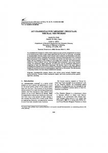
Fig. 1. Instant snapshots produced by the model (27), with a=1.6, c1 =0.28, and c2 =0.12. (a) t=5; (b) t=20; (c) t=75; (d) t=100.
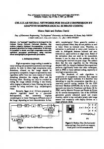
where φ is defined as the typical logistic map function φ ( x) = 1 − ax 2 , c1 and c2 are constants. In this study, the case where a=1.6, c1 =0.28, and c2 =0.12 was considered. Starting with an initial pattern of size 100 × 100 , where values of all the initial cells were randomly selected in [0,1], the model (27) was simulated. Some patterns are shown in Fig. 1. A dataset consisting of 2000 data pairs that were randomly selected from the first 100 patterns was created and this dataset was then used for GCNN model identification. A Gaussian white noise sequence with zero mean and standard deviation of 0.005 was added to the training dataset. Some conditions, relative to the model identification procedures using the PSO+OPP and FOR algorithms, are listed in Table 2. The ERS (error-to-signal ratio) criterion, relative to the PSO+OPP algorithm, is shown in Fig. 2. The adjustable generalised cross-validation (AGCV), defined by (26), is shown in Fig. 3, which suggests that a GCNN model with 31 model terms would be a good choice.
14
Table 2. Some conditions involved in the identification procedure. 100 × 100
Size of the arrays of cells Number of model variables mOPP in the OPP algorithm η in the OPP algorithm
9 200 10-5
Swarm size in the PSO algorithm c1, c2 in the PSO algorithm χ in the PSO algorithm
100 c1= c2=2.05 0.7298
mPSO in the PSO algorithm δ in the PSO algorithm ε in the FOR algorithm λ in the FOR algorithm
500 10-5 10-10 10
Fig. 2. The ESR(error-to-signal ratio) criterion, relative to the PSO+OPP algorithm.
Fig. 3. The AGCV criterion, relative to the FOR algorithm.
15
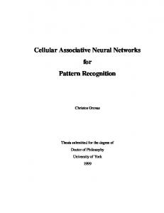
To evaluate the performance of the identified GCNN model of 31 model terms, the patterns produced by this model were investigated and compared with those produced by the original model (27). Denote the observation of the pattern measured at the time instant t by X(t). The k-step-ahead prediction, denoted by Xˆ (t + k | X (t ); f ) , where f represents the identified nonlinear function, is the iteratively produced result using the identified model, on the basis of X(t), but without using information on observations for patterns at any other time instants. As an example, starting with a random initial pattern of size 128 × 128 , where values were uniformly distributed in [0,1] , the one and ten step-ahead predicted patterns were calculated using the identified GCNN model. The one and ten step ahead predicted patterns at time instant t=20, along with the corresponding patterns produced by the model (26), are shown in Fig. 4, which clearly shows that the identified GCNN model can be used to reconstruct the dynamics possessed by the original model (27).
(a)
(b)
(c)
Fig. 4. A comparison of the 1- and 10-step-ahead predicted patterns at the time instant t=20, produced by the identified GCNN model, with that produced by the original model (27). (a) The pattern produced by the original model (27); (b) 1-step-ahead predicted pattern; (c) 10-step-ahead predicted pattern.
5. Conclusions The proposed generalized CNN (GCNN) modeling framework provides a powerful model identification approach for spatio-temporal evolutionary (STE) systems. The introduction of the novel two-stage training scheme, where the PSO based orthogonal projection pursuit (OPP) algorithm is employed for a coarse model identification and the mutual information assisted forward orthogonal regression (FOR) algorithm is used for model refinement, enable the GCNN modeling procedure to be very effective because of the following features. Firstly, the network training procedure is almost selfimplemented, meaning that by starting with some given conditions (initial, boundary and termination), all the within and between-network parameters can be estimated and calculated by the proposed
16
algorithms. Secondly, the model identification procedure can produce a transparent model, where individual neurons are explicitly available. Thirdly, by applying the FOR algorithm, the initially produced model by the OPP algorithm, can be significantly refined and improved, and a parsimonious model containing only a small number of neurons can then be obtained. By introducing the PSO algorithm, which is easy to implement, the calculation of gradients required by classical nonlinear optimisation algorithms can be avoided. This makes the new modelling framework very suitable for STE system identification, where relevant object functions may not be differentiable or relevant gradients are very difficult to obtain.
Acknowledgements The authors gratefully acknowledge that this work was supported by Engineering and Physical Sciences Research Council (EPSRC), U.K.
References Adamatzky, A. [1994] Identification of Cellular Automata (London: Taylor & Francis). Aguirre, L. A. & Billings, S. A. [1995] “Retrieving dynamical invariants from chaotic data using NARMAX models,” Int. J. Bifurcation and Chaos, 5, 449-474. Billings, S. A., Chen, S. & Korenberg, M. J. [1989] “Identification of MIMO nonlinear systems suing a forward regression orthogonal estimator,” Int. J. Control, 49, 2157-2189. Billings, S. A. & Yang, X. X. [2003] “Identification of the neighborhood and CA rules from spatiotemporal CA patterns,” IEEE Trans. Syst., Man, Cybern., B: Cybern., 33, 332–339. Billings, S. A. & Wei, H. L. [2005] “The wavelet-NARMAX representation: a hybrid model structure combining the polynomial models and multiresolution wavelet decompositions”, Int. J. Systems Science, 36, 137-152. Billings, S. A. & Wei, H. L. [2007a] “Sparse model identification using a forward orthogonal regression algorithm aided by mutual information,” IEEE Trans. Neural Networks, 18, 306-310. Billings, S. A. & Wei, H. L. [2007b] “An adaptive orthogonal search algorithm for model subset selection and nonlinear system identification,” Int. J. Control (in press). Billings, S. A. & Zhu, Q. M. [1994] “A structure detection algorithm for nonlinear dynamical rational models”, Int. J. Control, 59, 1439-1463. Cai, H. & Min, L. Q. [2005] “A kind of two-input CNN with application,” Int. J. Bifurcation and Chaos, 15, 4007-4011. Chen, S., Billings, S. A. & Luo, W. [1989] “Orthogonal least squares methods and their application to nonlinear system identification,” Int. J. Control, 50, 1873–1896. Chen, S., Hong, X. & Harris, C. J. [2003] “Sparse kernel regression modeling using combined locally regularized orthogonal least squares and D-optimality experimental design,” IEEE Trans. Automatic Control, 48, 1029-1036. 17
Chen, S., Hong, X., Harris, C. J. & Sharkey, P. M. [2004] “Sparse modeling using orthogonal forward regression with press statistic and regularization,” IEEE Trans. Syst., Man, Cybern., B: Cybern., 34, 898–911. Chen, F. J., Chen, F. Y. & He, G. L. [2005] “Image processing via CNN genes with Von Neumann neighborhoods,” Int. J. Bifurcation and Chaos, 15, 3999-4006. Chua, L. O. & Yang, Y. [1988a] “Cellular neural networks: Theory,” IEEE Trans. Circuits Syst. I, Fundam. Theory Appl., 35, 1257–1272. Chua, L. O. & Yang, Y. [1988b] “Cellular neural networks: Applications,” IEEE Trans. Circuits Syst. I, Fundam. Theory Appl., 35, 1273–1290. Chua, L. O. & Roska, T. [1993] “The CNN paradigm,” IEEE Trans. Circuits Syst. I, Fundam. Theory Appl., 40, 147–156. Chua, L. O., Hasler, M., Moschytz, G. S. & Neirynck, J. [1995] “Autonomous cellular neural networks - a unified paradigm for pattern-formation and active wave-propagation,” IEEE Trans. Circuits Syst. I, Fundam. Theory Appl., 42, 559-577. Chua, L. O. & Roska, T. [2002] Cellular Neural Networks and Visual Computing (Cambridge: Cambridge University Press). Clerc, M. & Kennedy, J. [2002] “The particle swarm-explosion, stability, and convergence in a multidimensional complex space,” IEEE Trans. Evol. Comput., 6, 58–73. Cover, T. M. & Thomas, J. A. [1991] Elements of Information Theory (New York: John Wiley & Sons). Crounse, K. R. & Chua, L. O. [1995] “Methods for image-processing and pattern-formation in cellular neural networks - a tutorial,” IEEE Trans. Circuits Syst. I, Fundam. Theory Appl., 42, 583-601. Crounse, K. R., Roska, T. & Chua, L. O. [1993] “Image half-toning with cellular neural networks,” IEEE Trans. Circuits Syst. II, Analog and Digital Signal Processing., 40, 267-283. Crounse, K. R., Chua, L. O., Thiran, P. & Setti, G. [1996] “Characterization and dynamics of pattern formation in cellular neural networks,” Int. J. Bifurcation and Chaos, 6, 1703-1724. Darbellay, G.A. & Vajda, I. [1999] “Estimation of the information by an adaptive partitioning of the observation space,” IEEE Transactions on Information Theory, 45, 1315-1321. Eberhart, R. C. & Kennedy, J. [1995] “A new optimizer using particle swarm theory,” in Proc. 6 th Symp. Micro Mach. Human Sci., pp.39-43, Nagoya, Japan, Oct. 4-6, 1995. Friedman, J. H. & Stuetzle, W. [1981] “Projection pursuit regression,” J. Amer. Statist. Assoc., 76, 817–823. Gilli, M., Roska, T., Chua, L. O. & Civalleri, P. P. [2002] “CNN dynamics represent a broader class than PDEs,” Int. J. Bifurcation and Chaos, 12, 2051-2068. Harrer, H. & Nossek, J. A. [1992] “Discrete0time cellular networks,” Int. J. Circuit Theory Applicat., 20, 453-467. He, Q. B. & Chen, F. Y. [2006] “Designing CNN genes for binary image edge smoothing and noise
18
removing,” Int. J. Bifurcation and Chaos, 16, 3007-3013. Huang, G. B., Chen, L. & Siew, C. K. [2006] “Universal approximation using incremental constructive feedforward networks with random hidden nodes,” IEEE Trans. Neural Networks, 17, 879–892. Hwang, J. N., Lay, S. R., Maechler, M., Martin, R. D. & Schimert, J. [1994] “Regression modeling in back-propagation and projection pursuit learning,” IEEE Trans. Neural Networks, 5, 342–353. Itoh, M. & Chua, L. O. [2003] “Equivalent CNN cell models and patters,” Int. J. Bifurcation and Chaos, 13, 1055-1161. Itoh, M. & Chua, L. O. [2005] “Image processing and self-organizing CNN,” Int. J. Bifurcation and Chaos, 15, 2939-2958. Jones, L. K. [1992] “A simple lemma on greedy approximation in Hilbert space and convergence rates for projection pursuit regression and neural network training,” Ann. Statist., 20, 608–613. Kanakov, O. I., Shalfeev, V. D. & Forti, G. L. [2006] “Stationary patterns in CNN-like ensembles with modified cell output functions,” Int. J. Bifurcation and Chaos, 16, 2207-2220. Kaneko, K. [1993] Theory and Application of Coupled Map Lattices (New York: Wiley). Kennedy, J. & Eberhart, R. C. [1995] “Particle swarm optimization,” in Proc.IEEE Int. Conf. Neural Networks, vol. IV, pp.1942–1948, Perth, Australia, 1995. J. Kennedy, R. C. Eberhart and Y. Shi, Swarm Intelligence, San Francisco: Morgan Kaufmann Publishers, 2001. Kwok, T. Y. & Yeung, D. Y. [1997a] “Constructive algorithms for structure learning in feedforward neural networks for regression problems,” IEEE Trans. Neural Netw., 8, 630–645. Kwok, T. Y. & Yeung, D. Y. [1997b] “Objective functions for training new hidden units in constructive neural networks,” IEEE Trans. Neural Netw., 8, 1131–1148. Lin, S. S. & Yang, T. S. [2002] “On the spatial entropy and patterns of two-dimensional cellular neural networks,” Int. J. Bifurcation and Chaos, 12, 115-128. Mallat, S. & Zhang, Z. [1993] “Matching pursuit with time-frequency dictionaries,” IEEE Trans. Signal Process., 41, 3397–3415. Miller, J. & Huse, D. A. [1993] “Macroscopic equilibrium from microscopic irreversibility in a chaotic coupled map lattice,” Phys. Rev. E 48, 2528–2535. Moddemeijer, R. [1989] “On estimation of entropy and mutual information of continuous distributions,” Signal Processing, 16, 233-246. Moddemeijer, R. [1999] “A statistic to estimate the variance of the histogram-based mutual information estimator based on dependent pairs of observations,” Signal Processing, 75, 51-63. Morfu, S. & Comte, J. C. [2004] “A nonlinear oscillators network devoted to image processing,” Int. J. Bifurcation and Chaos, 14, 1385-1394. Paninski, L. [2003] “Estimation of entropy and mutual information,” Neural Computation, 15, 11911253.
19
Roska, T. & Chua, L. O. [1992] “Cellular neural networks with nonlinear and delay-type template elements and nonuniform grids,” International Journal of Circuit Theory and Applications, 20, 469481, Roska, T. & Chua, L. O. [1993], “The CNN universal machine - an analogic array computer,” IEEE Trans. Circuits Syst. II, Analog Digital Sign. Proc., 40, 163–173. Sbitnev, V. I. & Chua, L. O. [2002] “Local activity criteria for discrete-MAP CNN,” Int. J. Bifurcation and Chaos, 12, 1227-1272. Shi, B. E. [2004] “Oriented spatio patter formation in a four layer CMOS cellular network,” Int. J. Bifurcation and Chaos, 14, 1209-1221. Shi, Y. & Eberhart, R. C. [1998a] “Parameter selection in particle swarm optimization,” in Lecture Notes In Computer Science, V. W. Porto, N. Saravanan, D. Waagen, and A. E. Eiben (Eds), 1447, 591-600. Shi, Y. & Eberhart, R. C. [1998b] “A modified particle swarm optimizer,” in Proc. IEEE Conf. Evolutionary Computation, 69-73, Anchorage, AK, USA, 4th -9th May, 1998. Stoffels, A., Roska, T. & Chua, L. O. [1996] “On object-oriented video coding using the CNN universal machine,” IEEE Trans. Circuits Syst. I, Fundam. Theory Appl., 43, 948-952. Thiran, P., Crounse, K. R., Chua, L. O. & Hasler, M. [1995] “Pattern-formation properties of autonomous cellular neural networks,” IEEE Trans. Circuits Syst. I, Fundam. Theory Appl., 42, 757774. van den Bergh, F. & Engelbrecht, A. P. [2004] “A cooperative approach to particle swarm optimization,” IEEE Trans. Evolutionary Computation, 8, 225-239. Venetianer, P. L., Werblin, F., Roska, T. & Chua, L. O. [1995] “Analogic CNN algorithms for some image compression and restoration tasks,” IEEE Trans. Circuits Syst. I, Fundam. Theory Appl., 42, 278-284. Wei, H. L. & Billings, S. A. [2004] “Identification and reconstruction of chaotic systems using multiresolution wavelet decompositions,” Int. J. Systems Science, 35, 511-526. Wei, H. L., Billings, S. A. & Liu, J. [2004] “Term and variable selection for nonlinear system identification,” Int. J. Control, 77, 86-110. Wei, H. L. & Billings, S. A. [2007], “Model structure selection using an integrated forward orthogonal search algorithm assisted by squared correlation and mutual information,” Int.J. Modelling, Identification and Control (in press). Wolfram, S. [2002] A New Kind of Science (Champaign, IL: Wolfman Media).
20