The double body is composed of two overlapping circles/spheres of arbitrary ...... the double sphere (composite bubble) formed by two overlapping unequal, ...
GENERALIZED CIRCLE AND SPHERE THEOREMS FOR INVISCID AND VISCOUS FLOWS PRABIR DARIPA∗ AND D. PALANIAPPAN DEPARTMENT OF MATHEMATICS TEXAS A&M UNIVERSITY COLLEGE STATION, TEXAS
77843-3368
Abstract. The circle and sphere theorems in classical hydrodynamics are generalized to a composite double body. The double body is composed of two overlapping circles/spheres of arbitrary radii intersecting at a vertex angle π/n, n an integer. The Kelvin’s transformation is used successively to obtain closed form expressions for several flow problems. The problems considered here include two-dimensional and axisymmetric three-dimensional inviscid and slow viscous flows. The general results are presented as theorems followed by simple proofs. The two-dimensional results are obtained using complex function theory while the three-dimensional formulas are obtained using Stokes stream function. The solutions for several flows in the presence of the composite geometry are derived by the use of these theorems. These solutions are in singularity forms and the image singularities are interpreted in each case. In the case of three-dimensional axisymmetric viscous flows, a Faxen relation for the force acting on the composite bubble is derived.
Key words. circle theorem, sphere theorem, inviscid flow, viscous flow, Kelvin’s transformation AMS(MOS) subject classifications. 76B99, 76D07, 76M25 Running head: Generalized Circle And Sphere Theorems 1. Introduction. The celebrated Kelvin’s transformation [10, 14, 16, 40] has been used frequently to determine the image system of a given potential distribution in the presence of a sphere or a circular cylinder. Applying Kelvin’s transformation, also known as Kelvin’s inversion theorem, on harmonic functions, Weiss [37] established a relation connecting the velocity potential of the irrotational flow of an incompressible inviscid fluid around a sphere with that of the flow when the sphere is absent. The corresponding theorem for axisymmetric flows was developed by Butler [6] in a simpler form using the Stokes stream function. The two-dimensional counterpart of the Weiss sphere theorem was obtained earlier by Milne-Thomson [23, 24] which is widely known as the circle theorem. These basic theorems were extended by several authors in order to satisfy various boundary conditions that arise in various fields such as hydrodynamics, heat, magnetism and electrostatics [19, 28, 29, 30, 38, 39]. The Kelvin’s inversion was the key idea in those works involving a single spherical or a circular boundary. The Kelvin’s inversion theorem is also applied to scattering problems of linear acoustics [11]. In addition, the Kelvin’s inversion theorem has been also generalized to the cases of biharmonic and polyharmonic functions [7]. In [12, 25, 26], the result for biharmonic function has been used to obtain sphere theorems for Stokes flows involving a spherical boundary under a variety of boundary conditions. The earlier sphere theorems for axisymmetric slow viscous flows [8, 9, 13] also used the inversion theorem implicitly. The circle theorems for Stokes flows [1, 35] further exploited the use of the inversion theorem for biharmonic functions. It is worth citing the notable extensions of circle and sphere theorems for isotropic elastic media [20, 5]. In this paper, we generalize the basic theorems to the case of a composite geometry consisting of two overlapping spheres/circles. The two spherical/cylindrical surfaces ∗ AUTHOR
FOR CORRESPONDENCE 1
2
Daripa and Palaniappan
are assumed to intersect at the vertex ‘P’ (see Fig. 2.1) at an angle π/n, n an integer. For our purposes, we call this angle ‘vertex angle’ in this paper. The chief advantage of this assumption is that Kelvin’s inversion can be used successively to obtain general expressions for the required functions satisfying the boundary conditions. This idea has been used here to present generalized circle and sphere theorems for inviscid and viscous flows. In a sense, this generalizes the idea that it is easier to construct images in wedges of angle π/n (n an integer) than when the angle is an irrational multiple of π. It should be pointed out that the problems involving overlapping circles/spheres are, in general, solved by the use of toroidal and bicylindrical coordinates [17, 18, 31, 32]. This method uses the conical functions and may become cumbersome while computing the results in general situations. Our present approach avoids such special coordinate systems making the derivation simple. We also mention that the method of electric inversion due to Maxwell [21] has been used in electrostatics to calculate the dipole moment for equal conducting spheres [15, 22]. The layout of the paper is as follows: In section 2, we describe the overlapping geometry and provide some nice properties of the geometrical relations. We first present the generalized circle theorem for inviscid flows in Section 3. The usefulness of this theorem is also demonstrated with several examples. In section 4, the corresponding theorem for Stokes flows is obtained. We have employed the inversion theorem for biharmonic functions to compute the stream function. For convenience, we have used the stress-free boundary conditions which yield simpler expressions. Here again, we present various examples to illustrate our general results. The theorem for inviscid axisymmetric flow about a sphere is provided in section 5. This may be considered as the extension of Butler’s sphere theorem for inviscid flows. The corresponding axisymmetric flow for two overlapping stress-free spherical surfaces is solved in section 6. The general expressions for the flow fields have been derived here for several cases and the drag force has been calculated in each of these cases. We finally conclude in section 7. 2. Geometry of the composite body. We consider two circles Sa and Sb of radii ‘a’ and ‘b’ centered at positions Sa and Sb respectively. The circles overlap as shown in Fig. 2.1, and intersect at an angle πn , n an integer. The distance ‘c’ between the centers is h π i1/2 c = a2 + b2 + 2ab cos . (2.1) n
The composite geometry consisting of two overlapping circles is called a double circle. The boundary of the double circle is denoted by Γ = Γa ∪ Γb , where Γa is part of the circle Sa and Γb is part of the circle Sb . Let Aj , Bj be the successive inverse points lying along the line joining the centers. The first point A1 is the image of B in circle Sa and B1 is the image of A in circle Sb . The successive image points starting with B are ordered as follows: B → A1 → B2 → A3 → B4 → A5 → B6 ..... Similarly, the successive image points starting with A are ordered as follows: A → B1 → A2 → B3 → A4 → B5 → A6 ..... The distances aj = AAj and bj = BBj satisfy the recurrence relations a2 aj = c − bj−1 , (2.2) 2 b bj = c − aj−1
3
Generalized Circle and Sphere Theorems
π π− n
Γa
Γb
P S
Sa
A
Bj
Aj
b
B
x-axis
Q
Fig. 2.1. Geometry of the double circle Γ.
with initial values a0 = b0 = 0 and j = 1, ..., n − 1. For the vertex angle integer, one can prove that (see Appendix) an−1 + bn−1 = c.
π n,
with n an (2.3)
In this case, the image points An−1 and Bn−1 coincide. The points {Aj } with j < (n − 1) lie inside circle Sa but outside the overlap region, and the points {Bj } with j < (n − 1) lie inside circle Sb but outside the overlap region. Such points exist only for n > 2. For n = 2, the first image points lie inside the overlap region and coincide. It can be further shown that the distances Aj P and Bj P (see Fig. 2.1) can be expressed in terms of aj and bj by � �1/2 2 2 2 b − a − c Aj P = (−1)j a2j + aj + a2 c , (2.4) � � 1/2 a 2 − b 2 − c2 2 j 2 bj + b Bj P = (−1) bj + c
with A0 P = AP = a, B0 P = BP = b. We note some further properties of the recurrence relations (2.2) and (2.4). By induction, one can prove from eq. (2.2) that the distances {aj , bj } are related by a2j b2j+1 = b2j a2j+1 . (2.5) a2 − b 2 a2j+1 − b2j+1 = c2
Using (2.5) in (2.4) one finds that
A2j+1 P = B2j+1 P. ′
(2.6)
Let z, z denote the complex positions of an arbitrary point with A and B as origins respectively. Similarly, let zj , zj′ denote the complex positions with Aj and Bj as origins respectively. Note that zj = z − zAj and zj′ = z − zBj , where zAj and zBj are the z-coordinates of the points Aj and Bj . Below, we discuss inviscid and viscous fluid flow problems involving the composite double body Γ separately.
4
Daripa and Palaniappan
3. Two-dimensional inviscid flow. Consider irrotational two-dimensional flows of incompressible inviscid fluids in the z-plane. Then the governing equations for the complex potential W (z) = φ + iψ is the two-dimensional Laplace’s equation which is written in complex form as ∂2W = 0, ∂z∂ z¯
(3.1)
where z = x + iy is the complex variable and z¯ its conjugate. The complex velocity may be obtained from u − iv =
dW . dz
(3.2)
If there are rigid boundaries present in the given flow field, then the boundary conditions can taken to be ψ = constant, different constants on different boundaries. Based on this formulation, Milne-Thomson [23, 24] presented an elegant theorem for the calculation of the flow disturbance resulting from the introduction of an infinite circular cylinder to a given two-dimensional flow field. It is widely known as the ‘circle theorem’. The theorem can also be used for non-circular boundaries if one can find conformal transformation that maps the given boundary to a circle. The circle theorem of Milne-Thomson has also its analogue in electrostatics [29], Stokes flows [1, 35] and in isotropic elasticity [20]. Furthermore, the circle theorem has also been extended to include surface singularity distributions [33, 2]. More recently, Bellamy-Knights [3] extended the circle theorem to the case of an elliptic cylinder, by the use of conformal mapping. The latter author gave a general expression for the image system in an elliptical cylinder and used it to calculate the source-sink surface singularity distribution on the ellipse. In the following, we state and prove a theorem for a double circle Γ, formed by two infinite circular cylinders overlapping at an angle π n , n an integer (see Fig. 2.1), introduced into the given potential flow field. Theorem 3.1. Let f (z) be the complex potential of the two-dimensional irrotational motion of the incompressible inviscid fluid in z-plane whose singularities (sources, vortices etc.) lie outside the double circle Γ. If we introduce an infinite cylinder Γ into the flow field of f (z) then the modified potential becomes W = f (z) + f1 (z),
f1 (z) = f¯
(3.3)
� b2 + c z′ � � n−1 X � Aj P 2 ′ f mod mod(j − 1, 2)AAj + mod(j, 2)ABj + (−1)j + zj j=1 !# Bj P 2 +f mod mod(j − 1, 2)ABj + mod(j, 2)AAj + (−1)j ′ (3.4) zj
�
a2 z
�
+ f¯
�
where the prime on summation indicates ( that the last term must be divided by 2, f, j odd f mod = ¯ f , j even,
5
Generalized Circle and Sphere Theorems
and mod(i, j) = integer part of (i/j). Proof. We first note that the image terms are obtained by the use of successive Kelvin’s inversion. It is known that the given harmonic function and its Kelvin’s inversion will have the same value on the boundary . This property can be used in showing how boundary conditions are satisfied. In view of this, it is sufficient to prove the above theorem for the special case n = 2 and the proof for any fixed integer n follows in a similar fashion. The expression (3.4) for n = 2 becomes � 2� � 2 � � � 2 a b a2 b 2 a f1 (z) = f¯ + f¯ ′ + c + f . (3.5) − 2 z z c c z1 The conditions to be satisfied are that (1) f1 (z) must be a solution of (3.1); (2) f1 (z) must have its singularities within Γ; (3) W = f (z) + f1 (z) must be real on Γ. Let us now proceed to show that f1 (z) given by (3.5) and hence W (z) satisfy the above conditions. ∂2 The operator ∂z∂ z¯ is form invariant under the translation of origin along the x-axis (real axis). We observe the following properties: � 2� (i) Inversion: If f0 (z) is a solution of (3.1), then so is f¯0 a . This is analogous z
to Kelvin’s inversion in three dimensions. (ii) Reflection: If f0 (z) is a solution of (3.1), then f0 (−z) is also a solution. (iii) Shifting of origin: If f0 (z) is a solution of (3.1), then f0 (z + h), where h is a constant, is also a solution. These properties are also true for the conjugate function. In view of the above properties, f1 (z) given by (3.5) satisfies the Laplace equation and hence condition (1) is satisfied. 2 2 2 2 It can be seen that if z lies outside Γ, then az , bz , ac2 zb1 all lie inside Γ and condition (2) is also satisfied. To prove (3), we first note the following relations from the Fig. 2.1 z = z ′ + c = z1 + z1 = z ′ +
b2 , c
a2 , c
c2 = a 2 + b 2 .
Also, we have (
a2 z ′ z¯′ on |z| = a, b2 z z¯ on |z ′ | = b. By the use of these relations we see that � 2 ′� � 2 ′� � 2� a z¯ a z a ¯ ¯ +f +f , W = f (z) + f z c¯ z1 cz1 c2 z1 z¯1 =
� 2� � 2� a a W = f (¯ z ′ + c) + f¯ + f¯(¯ z ′ + c) + f , z z¯
on |z| = a,
on |z ′ | = b.
(3.6)
(3.7)
From (3.6), and (3.7) it is clear that W is real on Γ and therefore condition (3) is also satisfied. This completes the proof of the theorem for n = 2.
6
Daripa and Palaniappan
In a similar way, the theorem can be proved for arbitrary integer n. By the use of continuous reflections on either circle, we have successfully obtained the general solution to the problem. It is important to note that the solution is found in the z-plane without recourse to conformal mapping techniques. If we set either a = 0 or b = 0 in the above theorem we obtain the result for a single circular cylinder. We now illustrate the theorem for the double circle with several examples. 3.1. A double circle Γ at incidence to a uniform stream. The complex potential for the flow at upstream is taken to be f (z) = U zeiα . Now the complete complex potential after the introduction of Γ into this flow field, by the use of the Theorem 1, is � � 2 b a2 + c e−iα W (z) = U zeiα + U e−iα + U z z′ n−1 X �� Aj P 2 ′ mod(j − 1, 2)AAj + mod(j, 2)ABj + (−1)j +U zj mod j=1 # ) 2 iα j Bj P e (3.8) + mod (j − 1, 2)ABj + mod(j, 2)AAj + (−1) ′ zj mod j mod where
(
zj , j odd z¯j , j even and similar definition holds for zj′ mod and the exponential appearing in the summa2 iα tion. The image system consists of doublets of strengths U Aj P 2 eiα j mod , U Bj P ej mod respectively located at the points Aj and Bj . In addition, there are constants corresponding to each image doublet appearing in the perturbed part of the complex potential. These constants appear due to geometrical asymmetry and are part of the solution. The boundary condition of the problem is satisfied with the aid of these constants. In order to exemplify the use of (3.8), we consider a special value for n, say n = 2. In this case, (3.8) becomes � � � 2 � 2 a2 −iα a2 b 2 a b iα −iα W (z) = U ze + U e eiα . (3.9) +c e +U +U − 2 z z′ c c z1 zj mod =
The image doublets in the present case are located at A, B and A1 (= B1 ) respectively. 2 2 The strengths of these doublets are U a2 e−iα , U b2 e−iα and −U ac2b eiα respectively. We notice from (3.9) that the constants make the W real on Γ and do not contribute anything to the complex velocity. The streamlines for uniform flow past the double circle are plotted for the cases n = 2 and n = 3 in Fig. 3.1(a)-(c). The flow streamlines are, as expected, curved near the spherical surfaces and straight everywhere else. The flow patterns in Fig. 3.1(d)-(f) are discussed in the next subsection. Fig. 3.2 shows instantaneous streamlines after the steady flow has been subtracted out. The instantaneous streamlines in this figure are very similar to those for a double source (dipole).
Generalized Circle and Sphere Theorems
7
The constants in the perturbed flow depend on the choice of origin. We may illustrate this by choosing the origin at the center of the line of intersection of the two circles. The complex potential may be obtained by the use of the theorem developed in section 3, with the distances AAj , BBj etc. properly defined with respect to the new origin. For simplicity we choose again n = 2 and the complete complex potential for the uniform flow is � � 2 � � 2 b a2 b2 a2 b2 iα a −iα −iα iα e . (3.10) − + e +U e − U W (z) = U z1 e + U z c z′ c c2 z 1 Comparing the above expression with (3.9), we notice that the image systems are the same but the constants are different. Interestingly, the constants in (3.10) cancel if the two circles have the same radii (i.e. a = b). This is due to the added symmetry about the y-axis. 3.2. Stagnation point flow. The complex potential in the absence of the cylinder is f (z) = kz 2 , where k is a constant. The complete complex potential in the presence of Γ is therefore, (by the use of the Theorem 1) � 2 �2 a4 b W (z) = kz 2 + k 2 + k + c z z′ " �2 n−1 X � Aj P 2 ′ mod(j − 1, 2)AAj + mod(j, 2)BBj + (−1)j +k zj mod j=1 !2 Bj P 2 . + mod(j − 1, 2)BBj + mod(j, 2)AAj + (−1)j ′ zj mod
The definitions of the notations are the same as before. The image system consists of quadrupoles at the points Aj and Bj and doublets at B0 , Aj and Bj (j > 1). In the present example also, the constants appear for the compensation of the boundary condition and are origin dependent. As explained in the previous example, the constants vanish for two equal circles if the origin of Γ is chosen at the center of line of intersection of the two circles. The pattern of streamlines do not seem to be affected noticeably due to various vertex angles (see Fig. 3.1(d)-(f)). 3.3. Potential-dipole outside Γ. The complex potential due to a potentialdipole of strength µ2 located at (0, −d) whose axis is along the positive y−direction is µ2 f (z) = , z1 + d where z1 is a complex position of a point with E1 (0, −d) as origin. The complex potential in the presence of a double circle, by the use of the Theorem 1, becomes ( 1 1 1 a2 b2 W (z) = µ2 − 2 − 2 z1 + d d z2 + a /d (c + d)2 z3 + b2 /d #) " n−1 X Bj P 2 Aj P 2 j ′ j (3.11) + (−1) ′ (−1) + zj mod + AAj zj mod + BBj j=1 The image system consists of dipoles at the image points Aj and Bj . The plots of streamlines in dipole flow are sketched in Fig. 3.3(a)-(b). It may be seen that
8
Daripa and Palaniappan
6
6
5
5
4
4
3
3
2
2
1
1
0 −6
−4
−2
0
2
4
6
8
10
12
0 −6
−4
−2
0
2
(a)
6
6
5
5
4
4
3
3
2
2
1
1
0 −6
−4
−2
0
2
4
6
8
10
12
0 −6
−4
−2
0
2
(b)
6
5
5
4
4
3
3
2
2
1
1 −4
−2
0
2
4 (c)
6
8
10
12
4
6
8
10
12
4
6
8
10
12
(e)
6
0 −6
4 (d)
6
8
10
12
0 −6
−4
−2
0
2 (f)
Fig. 3.1. Streamline patterns for two-dimensional potential flows for two vertex angles π/n and different radii ratio a/b. (i) Uniform flow: (a) n = 2, a/b = 2, (b) n = 3, a/b = 2, (a) n = 3, a/b = 1. (ii) Extensional flow:(d) n = 2, a/b = 2, (e) n = 3, a/b = 2, (f ) n = 3, a/b = 1.
9
Generalized Circle and Sphere Theorems
6
6
5
5
4
4
3
3
2
2
1
1
0 −6
−4
−2
0
2
4
6
8
10
12
0 −6
−4
−2
0
2
(a)
6
6
5
5
4
4
3
3
2
2
1
1
0 −6
−4
−2
0
2
4
6
8
10
12
0 −6
−4
−2
0
2
(b)
6
5
5
4
4
3
3
2
2
1
1 −4
−2
0
2
4 (c)
6
8
10
12
4
6
8
10
12
4
6
8
10
12
(e)
6
0 −6
4 (d)
6
8
10
12
0 −6
−4
−2
0
2 (f)
Fig. 3.2. Instantaneous streamlines after the steady flow has been subtracted out for two vertex angles and different radii ratio (Two-dimensional case): (i) n = 2: (a) a/b = 1, (b) a/b = 2, (c) a/b = 0.5. (ii) n = 3: (d) a/b = 1, (e) a/b = 2, (f ) a/b = 0.5.
10
Daripa and Palaniappan
6
6
5
5
4
4
3
3
2
2
1
1
0 −6
−4
−2
0
2
4
6
8
10
12
0 −6
−4
−2
0
2
(a)
6
6
5
5
4
4
3
3
2
2
1
1
0 −6
−4
−2
0
2
4
6
8
10
12
4
6
8
10
12
(b)
4
6
8
10
(c)
12
0 −6
−4
−2
0
2 (d)
Fig. 3.3. Streamline patterns due to potential dipole for two vertex angles and same radii ratio a/b = 1). (i) Two-dimensional case: (a) n = 2, d = a + 0.5, (b) n = 3, d = a + 0.5. (ii) Three-dimensional case: (c) n = 2, d = a + 1.0, (d) n = 3, d = a + 1.0.
the location of the singularity and the vertex angle do not change the flow pattern significantly. 4. Two-dimensional Stokes flow. We now consider the steady viscous flow around the double circle Γ. We assume that the Reynolds number is very small so that the inertial effects can be neglected. In the case of a steady, two-dimensional slow motion of a viscous incompressible fluid, it is convenient to use the stream function formulation. It is well-known that the stream function in this case satisfies the twodimensional biharmonic equation
∇4 ψ = 0.
(4.1)
Generalized Circle and Sphere Theorems
where ∇2 = are
∂2 ∂x2
+
∂2 ∂y 2 .
11
The velocity components in spherical polar coordinates (r, θ) 1 ∂ψ qr = − r ∂θ ∂ψ qθ = . ∂r
.
(4.2)
We define ψ(x, y) = Im[S(z, z¯)], where S is called a generalized stream function and satisfies the biharmonic equation (in complex form) ∂4S = 0. ∂z 2 ∂ z¯2
(4.3)
The problem now reduces to solving equation (4.3) subject to the boundary conditions prescribed on the double circle Γ. We select the boundary conditions on Γ as follows: • Normal velocity is zero on Γ; • Shear stress is zero on Γ. The above conditions make Γ a two-dimensional stationary composite bubble. A brief discussion on composite bubbles is provided in [4]. We now derive the above boundary conditions in terms of S. The zero normal velocity condition can be written in terms of S(z, z¯) (using (4.2)) as � S = 0 on z z¯ = a2 , . (4.4) S = 0 on z ′ z¯′ = b2 The stress-free conditions in terms of S may be derived as follows: The tangential stress component in polar coordinates is �
� 1 ∂qr ∂qθ qθ + − r ∂θ ∂r r � � 2 2 ∂ ψ 1 ∂ψ 1 ∂ ψ , − =µ − 2 2 + r ∂θ ∂r2 r ∂r
Trθ = µ
(4.5)
where µ is the dynamic coefficient of viscosity. Changing the variables from (r, θ) to z = reiθ and z¯ = re−iθ , we obtain the boundary condition Trθ = 0 on Γ as ∂2S ∂S z¯ − = 0 on z z¯ = a2 ∂z∂ z¯ ∂z , (4.6) 2 ∂ S ∂S z¯′ ′ ′ − ′ = 0 on z z¯ = b2 ∂z ∂ z¯ ∂z
where the suffix denotes partial differentiation. The governing equation (4.3) and the boundary conditions (4.4) and (4.6) constitute a well-posed problem whose solution provides the velocity and pressure prevailing in the presence of Γ. Now the general solution of (4.3) (in the absence of boundaries) is S(z, z¯) = f (z) + g(¯ z ) + zF (¯ z ) + z¯G(z)
(4.7)
where f (z), g(¯ z), F (¯ z ) and G(z) are analytic functions of their arguments. Therefore, two cases arise depending on whether the given flow is characterized by a harmonic
12
Daripa and Palaniappan
function f (z) or by a biharmonic function zF (¯ z ). In the following we present a theorem for calculating the perturbed flow when a stress-free double circle Γ is introduced into a given unbounded flow which may be either harmonic or biharmonic. Theorem 4.1. Let there be a two-dimensional slow viscous flow (Stokes flow or creeping flow) of an incompressible fluid in the z-plane. Let there be no boundaries and let the generalized complex stream function of the flow be a harmonic function f (z) (or a biharmonic function zF (¯ z )), whose singularities lie outside Γ. If a double circle Γ, consisting of two overlapping circles defined by |z| = a and |z ′ | = b which intersect at an angle nπ , n an integer, is introduced in the flow field satisfying the boundary conditions (4.4) and (4.6), then the generalized stream function S of the modified flow is given by (I)
(II)
� n−1 � 2� � X z z¯ z ′ z¯′ b2 a ′ (4.8) S(z, z¯) = f (z) − 2 f − 2 f c+ ′ + a z¯ b z¯ j=1 � � � 2 zj z¯j j Aj P f mod(x) mod(j − 1, 2)AAj + mod(j, 2)ABj + (−1) Ap P 2 zj !# ′ ′ 2 zj z¯j B P j f mod(x) mod(j − 1, 2)ABj + mod(j, 2)AAj + (−1)j ′ + Bj P 2 zj � 2� � � � � a cz ′ z¯′ b2 S(z, z¯) = zF (¯ z ) − zF − z′ + 2 F c+ ′ z b z �� � n−1 X zj z¯j ABj ′ zj mod + (−1)j − × Bj P 2 j=1 � � 2 j Aj P F mod(j − 1, 2)AAj + mod(j, 2)ABj + (−1) zj � � ′ ′ zj z¯j Bj A × + zj′ mod + (−1)j Aj P 2 !# 2 B P j F mod(j − 1, 2)ABj + mod(j, 2)AAj + (−1)j ′ (4.9) zj
where
(
f (x), j odd f (¯ x), j even and ( z¯j , jodd zj mod = zj , j even with similar definitions for zj′ mod . The other notations are the same as those defined in Section 3. Proof. We prove the result (4.8) for the case n = 2 and the proof for arbitrary integer n follows in a similar fashion. The expression (4.8) for n = 2 is � � � 2� � � 2 z ′ z¯′ c2 z1 z¯1 b2 a2 b 2 z a z z¯ − 2 f c+ ′ + 2 2 −f . (4.10) − 2 S(z, z¯) = f (z) − 2 f a z¯ b z¯ a b c c z1 f mod(x) =
The properties (i), (ii) and (iii) stated in Section 3 are also satisfied by equation (4.3) and therefore the perturbation terms in (4.10) are the solutions of (4.3).
Generalized Circle and Sphere Theorems
13
The singularities of the perturbed terms lie inside Γ because the singularities of the basic flow lie outside the double-circle. The condition (4.4) is satisfied by the use of the relations c2 z1 z¯1 = a2 z ′ z¯′ on |z| = a and c2 z z¯1 = b2 z z¯ on |z ′ | = b. The first condition in (4.6) on z z¯ = a2 yields � 2� � 2� � 2� a a a z¯ z¯ ′ ′ +f − f (z) + 2 f z¯Szz¯ − Sz = − 2 f a z¯ z¯ a z¯ � 2 � � � 2 b a z¯ + + ′ f′ c + ′ . cz1 z¯ z¯ Since c2 z1 z¯1 = a2 z ′ z¯′ on |z| = a, we see that r.h.s. of the above equation becomes zero. Similarly on |z ′ | = b, the second condition in (4.6) becomes � � � � � � � � b2 b2 z¯′ b2 b2 z¯′ ′ ′ ′ z¯ Sz′ z¯′ − Sz′ = − 2 f c + ′ + f c + ′ − f c + ′ + 2 c + ′ b z¯ z z¯ b z¯ � ′ � � 2 ′� z a z¯ b2 + f′ − z cz1 cz1 = 0 (since c2 z1 z¯1 = b2 z z¯ on z ′ z¯′ = b2 ).
Therefore all the necessary conditions are satisfied by the generalized stream function S given by (4.10). A similar proof of the result (4.9) may be established along the same lines. The theorem for a single circle may be obtained by setting one of the radii equal to zero. In the following we justify the usefulness of our theorem by considering various flow problems. 4.1. Stokes paradox. Consider the uniform motion of a fluid with speed U past a stress-free double circle Γ. The generalized stream function for the basic flow is f (z) = U z. The basic flow is characterized by a harmonic function. The generalized stream function for the modified flow may be constructed by the use of equation (4.8). Substituting f (z) = U z in (4.8), we obtain the result S(z, z¯) = 0.
(4.11)
The above result is the familiar ‘Stokes paradox’ which states that there is no solution for the uniform flow about a two-dimensional obstacle. The present results further confirm the validity of the paradox for intersecting circles. 4.2. Extensional flow. The basic flow is characterized by the harmonic func2 tion f (z) = αz2 , α is a shear constant. By the use of the expression (4.8) (of the Theorem 2 for the double circle), we obtain the generalized stream function for the perturbed flow as " � � α 2 a′ z b2 z ′ z¯′ z − S(z, z¯) = − 2 c + ′2 2 z¯ b z¯ ! n−1 4 X zj z¯j j Aj P ′ × mod(j − 1, 2)AAj + mod(j, 2)ABj + (1) 2 + Aj P 2 zj mod j=1 ! !# zj′ z¯j′ Bj P 4 + . (4.12) mod(j − 1, 2)ABj + mod(j, 2)AAj + (−1)j ′ 2 2 Bj P z j mod
14
Daripa and Palaniappan
It is of interest to analyze the stream function ψ corresponding to this flow. For convenient we consider the case when n = 2. The stream function ψ(r, θ) in polar coordinates is ψ(r, θ) = αr2 sin θ cos θ − αa2 sin θ cos θ − αb2 sin θ′ cos θ′ a2 a2 b 2 −αr′ c sin θ′ − α 2 sin θ1 cos θ1 + α r1 sin θ1 , c c
(4.13)
where (r, θ), (r′ , θ′ ) and (r1 , θ1 ) are the polar coordinates corresponding to z, z ′ and z1 , respectively. If we had chosen the origin at the circle of intersection then the modified stream function would have been ψ(r1 , θ1 ) = αr12 sin θ1 cos θ1 − αa2 sin θ cos θ − αb2 sin θ′ cos θ′ αa2 b2 a2 b2 − 2 sin θ1 cos θ1 + r sin θ − r′ sin θ′ . c c c
(4.14)
Note that the shifting of origin has altered the image terms. The last two terms correspond to the uniform flow at infinity and arise due to geometrical asymmetry. For two equal circles, these two terms cancel since r sin θ = r′ sin θ′ etc. The appearance of these terms is unusual and should be eliminated. For unequal circles one must subtract suitable terms from the perturbed solution in order to have a pure extensional flow at infinity. The above behavior may also arise in many circumstances. It appears that when the given flow is odd in z, the perturbed solution will have terms which produce uniform flow at infinity. By a suitable subtraction similar to that explained in the preceding paragraph, one might resolve the difficulties. The streamlines due to extensional flow for two different origin locations are plotted in Fig. 4.1(a)-(b). It may be noted that the change of origin does not alter the flow pattern. The streamlines in the present case are qualitatively similar to the two-dimensional inviscid flow past a double circle (Fig. 3.1(d)-(f)). 5. Three-dimensional inviscid flow. We consider two spheres of radii ‘a’ and ‘b’ centered at positions A and B respectively. Fig. 2.1 now represents the cross section of the two-sphere assembly in the meridian plane. The two spheres Sa and Sb overlap as shown in Fig. 2.1 and intersect at an angle πn , n an integer. The composite geometry Γ consisting of two overlapping spheres is called a double sphere. For the special case a = b it is called a dumbbell. The overlapping geometry also possesses the shape of a figure-eight lens. The following geometrical relations are evident from Fig. 2.1: π c2 = a2 + b2 + 2ab cos , n rj2 = r2 − 2AAj cos θ + AA2j , 2
= r′ + 2BAj cos θ′ + BA2j ,
(5.1)
(5.2)
where (r, θ, ϕ), (r′ , θ′ , ϕ) and (rj , θj , ϕ) are the spherical polar coordinates with respect to A, B and Aj respectively. The other geometrical relations provided in section 2 also hold for the present geometry. Therefore, we follow the notations used in section 2 in our present problem.
15
Generalized Circle and Sphere Theorems
6
6
5
5
4
4
3
3
2
2
1
1
0 −6
−4
−2
0
2
4
6
8
10
(a)
12
0 −6
−4
−2
0
2
4
6
(b)
Fig. 4.1. Streamline patterns for two-dimensional extensional creeping flows with different origins. (a) Origin at A (see Fig. 2.1), (b) Origin at the circle of intersection.
Consider axisymmetric irrotational flow of incompressible inviscid fluid in three dimensions. It is well-known that for an axisymmetric irrotational motion of an inviscid fluid, the Stokes stream function ψ(ρ, z), (ρ, z) being cylindrical coordinates, satisfies the equation D2 ψ = 0 2
2
(5.3)
∂ ∂ 1 ∂ where D2 = ∂ρ Since the operator D2 is form invariant under a 2 − ρ ∂ρ + ∂z 2 . translation of origin along the z-axis, we observe that: � 2 � 2 (A) Inversion: If ψ(ρ, z) is a solution of (5.3), then ar ψ ar2ρ , ar2 z is also a solution. This p is the known Kelvin’s inversion in a sphere whose radius is ‘a’. Here r = ρ2 + z 2 . (B) Reflection: If ψ(ρ, z) is a solution of (5.3), then so is ψ(ρ, −z). (C) Translation of origin: If ψ(ρ, z) is a solution of (5.3), then ψ(ρ, z + h), where h is a constant, is also a solution. We take z-axis as the axis of symmetry, and (ρ, z), (ρ′ , z ′ ), (ρj , zj ) and (ρ′j , zj′ ) as the cylindrical coordinates of a point outside Γ with A, B, Aj and Bj as origin. We now proceed to present a general theorem for constructing the perturbed stream function when the double sphere Γ is introduced into a given irrotational flow field. The problem of uniform flow about a lens (double sphere in our terminology) has been studied by many authors several years ago. The lens problem was treated by Shiffman and Spencer [36] by the use of an ingenious and difficult procedure involving the method of images in a multi-sheeted Riemann-Sommerfeld space. Later, a simple approach to the same problem was presented by Payne [27] by the use of generalized electrostatics. The latter author used the toroidal coordinates and Legendre functions of complex degree in the derivation of exact expressions for the stream function. However, the solutions derived in [36] and [27] involved tedious calculations and therefore only the problem of uniform flow around the lens was considered. Here we show that a simple general solution exists for arbitrary axisymmetric flow around a double sphere if the two spheres intersect at an angle nπ , n an integer. The method
8
10
12
16
Daripa and Palaniappan
is based on the Kelvin’s transformation which is taken successively n times. We show that The solution for the perturbed flow can be written down with the only knowledge of the stream function in an unbounded flow. The velocity components corresponding to the stream function ψ are given by 1 ∂ψ uρ = ρ ∂z (5.4) 1 ∂ψ . uz = − ρ ∂ρ
The boundary condition on Γ is that the normal velocity is zero on the surface. In terms of the stream function this condition becomes ψ=0
on Γ.
(5.5)
The above condition makes Γ a rigid boundary and the stream sheets are given directly. We denote by ψ0 (ρ, z) the stream function for an unbounded fluid motion. Theorem 5.1. Let ψ0 (ρ, z) be the Stokes stream function for an axisymmetric motion of an inviscid fluid in the unbounded region all of whose singularities lie outside the double sphere Γ, formed by two overlapping spheres which intersect at an angle π n , n an integer. When the rigid boundary Γ is introduced into the flow field of ψ0 , then the modified stream function for the fluid external to this boundary is given by � r � � a2 ρ a2 z � ψ0 ψ(ρ, z) = ψ0 (ρ, z) − , a r2 r2 � n−1 � ′� � 2 ′ X b ρ b2 z ′ r ′ ψ0 (−1)j+1 , c + ′2 + − ′2 b r r j=1 " ! 2 2 rj Aj P ρj j Aj P , mod(j + 1, 2)AAj + mod(j, 2)ABj + (−1) zj ψ0 Aj P rj2 rj2 Bj P 2 ′ ρ , mod(j + 1, 2)ABj r′2j j !!# 2 ′ j Bj P z + mod (j, 2)AAj + (−1) r′2j j
+
rj′ ψ0 Bj P
(5.6)
The notations are as defined in section 3. Proof. By virtue of the properties (A), (B) and (C), the perturbation terms in (5.6) are the solutions of (5.3). By the use of the geometrical relations (5.1) and (5.2), it can be shown that the expression (5.6) satisfies the boundary condition (5.5). Since the singularities of ψ0 (ρ, z) lie outside Γ, the singularities of the perturbation terms lie inside Γ. This is because the perturbation terms in (5.6) represent the inversion of ψ0 in Γ. Further, since ψ0 is finite at the origin, it�should be of order O(r2 ) there. Then the perturbation terms in (5.6) are of order O r1 for large r. This makes the perturbation velocity zero as r → ∞. Therefore, all the required conditions are satisfied by the expression (5.6). We note that the expression (5.6) represents a general solution to the stream function due to the presence of Γ in an axisymmetric, inviscid flow. This solution can be used as a basic set for the study of interactions of double sphere with other
Generalized Circle and Sphere Theorems
17
objects. Also, the solution has been obtained without the use of toroidal coordinates. If we set one of the radii of the spheres equal to zero, we recover the theorem for a single spherical boundary. In the following we present some examples to justify the usefulness of the theorem. 5.1. Uniform flow around Γ . The stream function for uniform flow along z−direction with the speed U is ψ0 = 12 U ρ2 . The perturbed stream function due to the presence of Γ may be obtained by the use of (5.6) and is given by ψ(ρ, z) =
1 2 1 a3 2 1 b3 ′2 U ρ − U 3 ρ − U ′2 ρ 2 2 r 2" r # n−1 3 X 1 Bj P 3 ′2 ′ j+1 Aj P 2 + U (−1) ρ + ′3 ρ j . 2 j−1 rj3 j rj
(5.7)
The image system consists of doublets (potential-dipoles) of strengths U a3 , U b3 , (−1)j+1 U Aj P 3 and (−1)j+1 U Bj P 3 located at A, B, Aj and Bj respectively. The distances Aj P and Bj P may be calculated by the use of the relations (2.4). The streamlines for the uniform flow are sketched in Fig. 5.1(a)-(c). The flow patterns are qualitatively similar to the two-dimensional inviscid flow (see Fig. 3.1(a)-(c)). Fig. 5.2 shows instantaneous streamlines after the steady flow has been subtracted out. These differ considerably from the two-dimensional motion (see Fig. 3.2). It may be of interest to analyze the expression for sum of the strengths of the image doublets, which is given by n−1 X ′ Dsum = −U a3 + b3 − (−1)j+1 (Aj P 3 + Bj P 3 ) . (5.8) j=1
The doublet strength can further be used to determine the virtual mass if the volume of the double sphere is known. The volume of the double sphere is � � 3(a − b)2 π 2a + 2b − c + (a + b + c)2 , (5.9) V = 12 c where c is given in (5.1). The virtual mass M now becomes M = πDsum − V,
(5.10)
where Dsum and V are given in (5.8) and (5.9). The plots of M V for various vertex decreases for b/a < 1 until angles are presented in Fig. 5.3. It can be seen that M V it reaches its minimum value. For the values b/a > 1, it increases gradually until it becomes a constant. The vertex angle has significant influence on the minimum value of M V . 5.2. Extensional flow. The stream function corresponding to the extensional flow (without Γ) is ψ0 = ρ2 z. The perturbed stream function, using (5.6), is � � n−1 X a5 ρ2 z b2 z b3 2 2 ′ ψ(ρ, z) = ρ z − (−1)j+1 (5.11) − 3ρ c+ 2 + 5 r r r j=1 " ! 2 Aj P 3 2 j Aj P ρ mod(j + 1, 2)AAj + mod(j, 2)ABj + (−1) zj rj3 j rj2 !# 2 Bj P 3 ′2 j Bj P ′ z . + ′ 3 ρ j mod(j + 1, 2)ABj + mod(j, 2)AAj + (−1) rj r′ 2j j
18
Daripa and Palaniappan
6
6
5
5
4
4
3
3
2
2
1
1
0 −6
−4
−2
0
2
4
6
8
10
12
0 −6
−4
−2
0
2
(a)
6
6
5
5
4
4
3
3
2
2
1
1
0 −6
−4
−2
0
2
4
6
8
10
12
0 −6
−4
−2
0
2
(b)
6
5
5
4
4
3
3
2
2
1
1 −4
−2
0
2
4 (c)
6
8
10
12
4
6
8
10
12
4
6
8
10
12
(e)
6
0 −6
4 (d)
6
8
10
12
0 −6
−4
−2
0
2 (f)
Fig. 5.1. Streamline patterns for three-dimensional potential flows for two vertex angles π/n and different radii ratio a/b. (i) Uniform flow: (a) n = 2, a/b = 2, (b) n = 3, a/b = 2, (c) n = 3, a/b = 1. (ii) Extensional flow:(d) n = 2, a/b = 2, (e) n = 3, a/b = 2, (f ) n = 3, a/b = 1.
19
Generalized Circle and Sphere Theorems
6
6
5
5
4
4
3
3
2
2
1
1
0 −6
−4
−2
0
2
4
6
8
10
12
0 −6
−4
−2
0
2
(a)
6
6
5
5
4
4
3
3
2
2
1
1
0 −6
−4
−2
0
2
4
6
8
10
12
0 −6
−4
−2
0
2
(b)
6
5
5
4
4
3
3
2
2
1
1 −4
−2
0
2
4 (c)
6
8
10
12
4
6
8
10
12
4
6
8
10
12
(e)
6
0 −6
4 (d)
6
8
10
12
0 −6
−4
−2
0
2 (f)
Fig. 5.2. Instantaneous streamlines after the steady flow has been subtracted out for two vertex angles and different radii ratio (Three-dimensional case): (i) n = 2: (a) a/b = 1, (b) a/b = 2, (c) a/b = 0.5. (ii) n = 3: (d) a/b = 1, (e) a/b = 2, (f ) a/b = 0.5.
20
Daripa and Palaniappan
1 n=2 n=3 n=4
0.98 0.96 0.94 M V
0.92 0.9 0.88 0.86 0
1
2
3
4
5
b/a Fig. 5.3. The virtual mass versus b/a.
The image system consists of potential quadrupoles of strengths a5 , b5 , (−1)j+1 Aj P 5 , (−1)j+1 Bj P 5 at A, B, Aj and Bj respectively. In addition, there are doublets located at B, Aj and Bj in the image system. The strengths of these doublets depend on the choice of coordinate system. For instance, if the origin is chosen at the center of the circle where the two spheres intersect, and further if a = b (equal spheres), the sum of the strengths of those doublets vanish. The streamlines in this case are qualitatively similar to those in the two-dimensional flow (see Fig. 5.1(d)-(e)). The vertex angle and the radii of the spherical surfaces do not change the flow pattern noticeably. 5.3. Potential-doublet. Now consider a potential-doublet of strength µ3 located at (0, 0, −d) on the axis of symmetry. The stream function corresponding to this doublet in the unbounded flow is ψ0 = µ3
ρ2 , r13
where r12 = r2 + 2dr cos θ + d2 . The complete stream function after the introduction of the double sphere, using the Theorem 3, becomes ψ(ρ, z) = µ3 ρ +
n−1 X j−1
2
′
"
−
a3 b3 − d3 r3 (c + d)3 r′2
(−1)j+1
Bj P 3 Aj P 3 + ′3 3 rj rj
!#
.
(5.12)
The image system consists of doublets at the respective image points. The streamline patterns in the present case are plotted in Fig. 3.3(c)-(d). Here again the location of dipole and vertex angle do not affect the flow structure.
Generalized Circle and Sphere Theorems
21
6. Three-dimensional Stokes flow. We consider a steady creeping flow of an incompressible viscous fluid in three dimensions. For an axisymmetric flow, the problem may be formulated in terms of Stokes stream function. In this case, the equations of motion reduce to solving the fourth order axisymmetric biharmonic equation D4 ψ = 0, 2
(6.1) 2
∂ ∂ 1 ∂ where, as in the previous section, D2 = ∂ρ 2 − ρ ∂ρ + ∂z 2 , (ρ, z) being cylindrical coordinates. Since z does not occur explicitly in the operator D2 , it is form invariant under a translation of origin along the z-axis. As in inviscid flow, we observe the following properties for the axisymmetric biharmonic equation: � � �3 2 2 (A’) Inversion: If ψ(ρ, z) is a solution of (6.1), then ar ψ ar2ρ , ar2z is also a solution. This is the well-known spherical inversion for biharmonic functions. p Here ‘a’ is the radius of inversion and r = ρ2 + z 2 . (B’) Reflection: If ψ(ρ, z) is a solution of (6.1), then, so is ψ(ρ, −z). (C’) Translation: If ψ(ρ, z) is a solution of (6.1), then ψ(ρ, z + h), where h is a constant, is also a solution. Note that the last two properties are the same as in the case of inviscid flow in three dimensions. We now derive the stream function when the double sphere Γ is introduced in to a given Stokes or creeping flow. There are several types of boundary conditions that may be imposed on Γ. We select the impervious and stress-free conditions on the surface. In terms of stream function they are stated as follows: (i) normal velocity is zero on Γ (impervious condition): � ψ = 0 on r = a (6.2) ψ = 0 on r′ = b
(ii) shear-stress is zero on Γ: � � 1 ∂ψ ∂ =0 on r = a ∂r �r2 ∂r � 1 ∂ψ ∂ = 0 on r′ = b. ∂r′ r′2 ∂r′
(6.3)
The conditions (6.2) make Γ a stream surface and (6.3) make it stress-free (composite bubbles). The existence of composite bubbles in liquids was discovered by Plateau who also discussed those observations in his book ‘Statique des Liquides’. Further brief discussion on composite bubbles is provided in [4]. The governing equation (6.1) subject to the boundary conditions (6.2) and (6.3) constitute a well-posed problem whose solution provides the velocity and pressure in the presence of the stress-free double sphere Γ. The velocity components may be obtained from (5.4) and the pressure may be found from ∂p µ ∂ =− (D2 ψ) ∂ρ ρ ∂z ∂p µ ∂ = (D2 ψ) ∂z ρ ∂p
(6.4)
where µ is the dynamic coefficient of viscosity. In the following, we state and prove a theorem for a composite bubble suspended in an arbitrary axisymmetric slow viscous flow.
22
Daripa and Palaniappan
Theorem 6.1. Let ψ0 (ρ, z) be the Stokes stream function for an axisymmetric motion of a viscous fluid in the unbounded region all of whose singularities lie outside the double sphere (composite bubble) formed by two overlapping unequal, impervious, shear-free spheres, intersect at an angle πn , n an integer, and suppose that ψ0 (ρ, z) = O(r2 ) at the origin. When the stress-free boundary Γ is introduced into the flow field of ψ0 , the modified stream function for the fluid external to Γ is ψ(ρ, z) = ψ0 (ρ, z) − "�
� r �3
�3
a
ψ0
�
a2 ρ a2 z , r2 r2
�
−
� ′ �3 � 2 ′ � n−1 X b ρ r b2 z ′ ′ (−1)j+1 + ψ0 , c + ′2 ′2 b r r j=1
Aj P 2 ρj , mod(j + 1, 2)AAj rj2 ! � �3 2 rj′ j Aj P zj + ψ0 + mod (j, 2)ABj + (−1) rj2 Bj P rj Aj P
ψ0
Bj P 2 ′ Bj P 2 ρj , mod(j + 1, 2)ABj + mod(j, 2)AAj + (−1)j ′ 2 zj′ 2 ′ rj rj
!#
.
(6.5)
Here again the notations are the same as those defined in section 3. The second and third terms on the r.h.s of (6.5) are the images of ψ0 (ρ, z) in the spheres A and B respectively and the terms in the summation represent the successive images. Proof. By virtue of the properties (A’), (B’) and (C’), the perturbation terms in (6.5) are the solutions of the axisymmetric biharmonic equation (6.1). It can be shown that the expression (6.5) satisfy the boundary conditions (6.2) and (6.3) by the use of relations (5.1) and (5.2). The perturbation terms in (6.5) have their singularities inside Γ since the singularities of ψ0 (ρ, z) lie outside the double sphere. Finally, since ψ0 (ρ, z)= o(r2 ) as r → 0, the perturbation terms in (6.5) are at most of order o(r) as r → ∞. Hence, the perturbation velocity tends to zero as r → ∞. This completes the proof. The above theorem may be used to compute the velocity and pressure fields when a stress-free boundary Γ is suspended in an arbitrary axisymmetric creeping flow. Our theorem reduces to the case of a single stress-free sphere if we set either a or b equal to zero. It is of interest to calculate the force on Γ in each case. Although the expression (6.5) may still be used to deduce the drag on the composite bubble, we give here another simple formula for finding the force without calculating the perturbed flow. We note that we employed the successive reflection technique in obtaining the perturbed stream function (6.5). By the use of the same procedure for the force, we obtain n−1 X ′ F = 4πµˆ ez a[u0 ]A + b[u0 ]B + (−1)j (Aj P [u0 ]Aj + Bj P [u0 ]Bj ) . (6.6) j=1
The expression (6.6) is a Faxen relation for the composite bubble. If one is interested in the force acting on Γ suspended in an axisymmetric flow, then (6.6) may be used without calculating the detailed flow. In the expression (6.6), eˆz is the unit vector in z direction, u ¯0 is the unperturbed flow and the suffixes outside the square brackets denote the evaluation of the quantities at those points. It is worth mentioning here that the drag force is equivalent to the strength of the image stokeslets. Therefore, if the solution in the presence of any body is expressed in singularity form, then the
23
Generalized Circle and Sphere Theorems
drag follows immediately from the image stokeslets strengths. The latter could be an alternative approach for the calculation of the drag force. 6.1. Uniform flow past Γ . The stream function for the uniform flow along the z-direction is ψ0 (ρ, z) = 12 U ρ2 . When the stress-free double sphere Γ is introduced in the flow field, then the modified stream function becomes (using (6.5)), ! n−1 Aj P 2 Bj P ′2 1 X′ ρ2 1 ρ′2 1 2 1 j+1 (−1) ρ + ′ ρj . ψ(ρ, z) = U ρ − U a − U b ′ + U 2 2 2 2 r 2 j=1 rj j rj
(6.7)
The image system consists of Stokeslets directed along z axis whose strengths are 4πµU a, 4πµU b, 4πµU (−1)j Aj P , 4πµU (−1)j Bj P located at A, B, Aj and Bj respectively. The streamlines for uniform flow past Γ are presented in Fig. 6.1(a)-(c). The flow patterns are as expected. The vertex angle and the radii of the spherical surfaces do not seem to influence the flow behavior. The drag may be calculated by the use of (6.6) and is given by n−1 X ′ F = 4πµUˆ ez a + b + (−1)j (Aj P + Bj P ) . (6.8) j=1
If we set either a = 0 or b = 0 in the above expression, we obtain the result for a single stress-free sphere. Fz The normalized drag 4πµu(a+b) is plotted against the ratio b/a) for various vertex angles in Fig. 6.2. Here, Fz is the z component of the force F. The graph shows that for each vertex angle, the drag force decreases monotonically with increasing b/a until it reaches a minimum at b/a ≈ 1, and thereafter it increases monotonically with increasing b/a. Thus, the drag attains its minimum value when the two spheres have almost the same radii, and this minimum value for the drag increases with increasing values of n, or equivalently, with decreasing vertex angle pi/n. 6.2. Extensional flow. The stream function for the extensional flow in the absence of Γ is ψ0 (ρ, z) = αρ2 z where α is a shear constant. The perturbed stream function due to the presence of Γ is ψ(ρ, z) = αρ2 z − αa3 "
hρ2 ρ2 z −α ′ 3 r r
� � n−1 X b2 z ′ ′ c + ′2 + α (−1)j+1 r j=1
Aj P 2 mod(j + 1, 2)AAj + mod(j, 2)ABj + (−1) zj rj2 !# 2 ′ j Bj P z . mod(j + 1, 2)ABj + mod(j, 2)AAj + (−1) r′ 2j j
Aj P 2 ρ rj j
j
!
+
Bj P ′2 ρj rj′ (6.9)
The image system consists of symmetric Stokes doublets (stresslets) of strengths αa3 , αb3 , α(−1)j Aj P 3 , α(−1)j Bj P 3 located at A, B, Aj and Bj respectively. In addition to these stresslets, there are Stokeslets at B, Aj and Bj respectively. The typical streamline pattern due to extensional flow in the presence of Γ are depicted in Fig. 6.1(d)-(e). The flow structure is similar to that in the case of inviscid flow (see Fig. 3.1(d)-(f)). The presence of the Stokeslets indicate that the stress-free double
24
Daripa and Palaniappan
6
6
5
5
4
4
3
3
2
2
1
1
0 −6
−4
−2
0
2
4
6
8
10
12
0 −6
−4
−2
0
2
(a)
6
6
5
5
4
4
3
3
2
2
1
1
0 −6
−4
−2
0
2
4
6
8
10
12
0 −6
−4
−2
0
2
(b)
6
5
5
4
4
3
3
2
2
1
1 −4
−2
0
2
4 (c)
6
8
10
12
4
6
8
10
12
4
6
8
10
12
(e)
6
0 −6
4 (d)
6
8
10
12
0 −6
−4
−2
0
2 (f)
Fig. 6.1. Streamline patterns for three-dimensional creeping flows for two vertex angles π/n and different radii ratio a/b. (i) Uniform flow: (a) n = 2, a/b = 2, (b) n = 3, a/b = 2, (a) n = 3, a/b = 1. (ii) Extensional flow:(d) n = 2, a/b = 2, (e) n = 3, a/b = 2, (f ) n = 3, a/b = 1.
25
Generalized Circle and Sphere Theorems
1 n=4 n=3 n=2
0.95 0.9 0.85 Fz 4πµU(a+b)
0.8
0.75 0.7 0.65 0.6 0
1
2
3
4
5
b/a Fig. 6.2. The variation of the drag force with the radii ratio b/a in uniform flow.
sphere Γ experiences a force in extensional flow. The force is found (using (6.6)) to be � n−1 X ′ (−1)j [Aj P (mod(j + 1, 2)AAj + mod(j, 2)ABj ) F = 4πµαˆ ez bc + j=1
� +Bj P (mod(j + 1, 2)ABj + mod(j, 2)AAj )] .
(6.10)
Fz In Fig. 6.3, the normalized drag 4πµα(a+b) 2 is plotted against the radii ratio b/a for various values of n. It is seen that the drag is monotonically increasing with b/a for each value of n. It appears from this figure that the rate of increase of the drag force decreases with increasing b/a, and the drag force appears to approach asymptotically to a constant value for large b/a, this constant being different for different n perhaps. Furthermore, we see that the drag increases with increasing n for each b/a. We note that the drag force in extensional flow is origin dependent. This is because the basic flow itself is origin dependent. If we choose the origin at the center of circle of intersection of the two spheres, then the force is zero if the two spheres have the same radii (i.e. a = b). This is due to the added symmetry in the problem. On the other hand if the spheres have different radii, the force does not become zero for any value of the parameters. If one wishes to calculate the stresslet coefficient, it is necessary to subtract the translational velocity obtained from Stokes problem. In this case, the translational part arising from extensional flow cancels with the translational part of the Stokes problem leaving out only stresslets in the solution. F3 located at 6.3. Stokeslet outside Γ. Consider a stokeslet of strength 8πµ (0, 0, −d) on the axis of symmetry. The stream function corresponding to this stokeslet
26
Daripa and Palaniappan
0.9 n=4 n=3 n=2
0.8 0.7 0.6 Fz 4πµα(a+b)2
0.5 0.4 0.3 0.2 0.1 0 0
2
4
6
8
10
b/a Fig. 6.3. The variation of the drag force with the radii ratio b/a in extensional flow.
in the unbounded flow is ψ0 =
F3 ρ2 , 8πµ r1
The complete stream function after the introduction of Γ, using the Theorem 4, becomes " a b F3 2 ρ − − ψ(ρ, z) = 8πµ dr (c + d)r′ � �# n−1 X Aj P Bj P ′ j+1 (−1) + . (6.11) + ′ rj rj j−1 The image system consists of stokeslets located at the respective image points. The streamline patterns in the present case are plotted in Fig. 6.4(a)-(d). Here again the location of stokeslet and vertex angle do not affect the flow structure. The force on the composite bubble in the present case, using (6.6), is a
n−1
X b ′ F = 4πµˆ ez (−1)j + + d c + d j=1
�
� Aj P Bj P + AAj BBj
(6.12)
z In Fig. 6.5, we have plotted the drag force 2F F3 , F3 = 8πµ against the radii ratio b/a for different vertex angles. The force increases or decreases according to b/a < or > 1. When b/a = 1, the drag attains its maximum value. Furthermore, the maximum value for the drag increases with decreasing value of n or equivalently, with increasing vertex angle π/n.
27
Generalized Circle and Sphere Theorems
6
6
5
5
4
4
3
3
2
2
1
1
0 −6
−4
−2
0
2
4
6
8
10
12
0 −6
−4
−2
0
2
(a)
6
6
5
5
4
4
3
3
2
2
1
1
0 −6
−4
−2
0
2
4 (b)
4
6
8
10
12
4
6
8
10
12
(c)
6
8
10
12
0 −6
−4
−2
0
2 (d)
Fig. 6.4. Streamline patterns due to a stokeslet located outside Γ for two vertex angles and same radii ratio a/b = 1. (a) n = 2, d = a + 1.0, (b) n = 3, d = a + 1.0, (c) n = 2, d = a + 0.5, (d) n = 3, d = a + 0.5.
7. Conclusion. Simple theorems are obtained for the two overlapping circles/spheres applicable to inviscid and viscous hydrodynamics. The key idea used in the derivation of our results is the Kelvin’s transformation. The present results cover the cases of single and two touching spherical/cylindrical surfaces, although, the latter has not been stated explicitly in the text. Our method does not use the toroidal or bicylindrical coordinates as in [27, 36] and hence avoids the tedious calculations even in complex flow situations. Another significant feature of our procedure is that it allows the interpretation of image singularities in each case. The locations of image singularities depend on the given potential distribution. Finally, the present results are constructed using the constraint that the two spherical/cylindrical surfaces intersect at a vertex angle π/n, n an integer. For an arbitrary vertex angle, the number of image terms may not terminate and one could end up with infinite terms. The toroidal or bicylindrical systems could be used in these situations but the resulting analysis could be as tedious as in the case of calculations with bispherical coordinates [34]. Furthermore, solving singularity driven flow
28
Daripa and Palaniappan
0.435 n=4 n=3 n=2
0.43 0.425 0.42 2Fz F3
0.415 0.41 0.405 0.4 0.395 0
1
2
3
4
5
b/a Fig. 6.5. The variation of the drag force with the radii ratio b/a due to a stokeslet.
problems using these coordinate systems is yet to be examined. Two- and three-dimensional flow patterns in uniform and extensional flows presented for several values of vertex angle show that the vertex angle does not influence the flow patterns significantly. These studies have been carried out subject to the constraint that the vertex angle be nπ . However, from our above studies it is presumably safe to conjecture that the flow pattern may not change noticeably even in the case of an arbitrary vertex angle. Appendix. Results in support of equation (2.3). The recurrence relations (2.2) for some special values of n are as follows: a2 , c
b1 =
a2 c , − b2
b2 =
a2 (c2 − a2 ) , c(c2 − a2 − b2 )
b3 =
a1 =
a2 =
a3 =
c2
a2 c(c2 − a2 − b2 ) �, a4 = � 2 2 2 2 2 2 2 c (c − a − b ) − b (c − b )
b2 c
c2
b2 c − a2
b2 (c2 − b2 ) c(c2 − a2 − b2 )
b4 = �
b2 c(c2 − a2 − b2 ) c2 (c2
−
a2
−
� � a2 c2 (c2 − a2 − b2 ) − a2 (c2 − a2 )
b2 )
�, a5 = � 2 2 2 2 2 2 2 2 c (c − b )(c − a − b ) − a (c − a )
−
a2 (c2
−
�
a2 )
Generalized Circle and Sphere Theorems
29
� � b2 c2 (c2 − a2 − b2 ) − b2 (c2 − b2 )
� b5 = � 2 2 2 2 2 2 2 2 c (c − a )(c − a − b ) − b (c − b ) Using the above expressions together with (2.1), it can be easily seen that an−1 + bn−1 = c for n = 2, 3, 4, 5, 6. In a similar way, it can be shown that this result is true for higher values of n also leading to the equation (2.3). 8. Acknowledgments. The authors are grateful to two anonymous referees, whose comments and suggestions improved the original version of the paper. This research has been partially supported by the interdisciplinary research program of the Office of the Vice President for Research and Associate Provost for Graduate Studies under grant IRI-98. REFERENCES [1] A. Avudainayagam and B. Jothiram, A circle theorem for plane Stokes flows, Q. Jl. Mech. Appl. Math., 41 (1986), pp. 383-393. [2] P. G. Bellamy-Knights, M. G. Benson, J. H. Gerrard and I. Gladwell, Analytical surface singularity distributions for flow about cylindrical bodies, J. Engg. Math., 23 (1989), pp. 261-271. [3] P. G. Bellamy-Knights, An image system and surface singularity solutions for potential flow past an elliptical cylinder, IMA J. Appl. Math., 15 (1998), pp. 299-310. [4] C. V. Boys, Soap bubbles and the forces which mold them, Dover, (1959). [5] J. H. Bramble, A sphere theorem for the equations of elasticity, Z. Angew. Math. Phys., 12 (1961), pp. 1-6. [6] S. F. J. Butler, A note on Stokes stream function for motion with spherical boundary, Proc. Cambridge Philos. Soc., 49 (1953), pp. 169-174. [7] A. T. Chwang, On spherical inversions of polyharmonic functions, Quart. Appl. Math., XLIV (1987), pp.793-799. [8] W. D. Collins, A note on Stokes stream function for the slow steady motion of viscous fluid before plane and spherical boundaries, Mathematika, 1 (1954), pp.125-130. [9] W. D. Collins, Note on a sphere theorem for the axisymmetric Stokes flow of a viscous fluid, Mathematika, 5(1958), pp.118-121. [10] R. Courant and D. Hilbert, Methods of Mathematical Physics (Interscience, New York, 1962), Vol. 2, pp. 242-246 and 286-290. [11] G. Dassios and R. E. Kleinman, On Kelvin inversion and low-frequency scattering, SIAM Review, 31 (1989), pp. 565-585. [12] J. F. Harper, Axisymmetric Stokes flow images in spherical free surfaces with applications to rising bubbles, J. Austral. Math. Soc. Ser. B, 25 (1983), pp. 217-231. [13] H. Hasimoto, A sphere theorem on the Stokes equation for axisymmetric viscous flow, J. Phys. Soc. Japan, 11 (1956), pp. 793-797. [14] J. H. Jeans, The Mathematical Theory of Electricity and Magnetism (Cambridge University Press, Cambridge, U.K., 1925). [15] T. B. Jones, Effective dipole moment of intersecting conducting spheres, J. Appl. Phys., 62 (1987), pp. 362-365. [16] O. D. Kellogg, Foundations of Potential Theory (Springer, Berlin, 1929), pp. 231-233 and 251-253. [17] N. N. Lebedev, I. P. Skalskaya, and Y. S. Uflyand, Problems of Mathematical Physics (PrenticeHall, Englewood Cliffs, NJ, 1965). [18] N. N. Lebedev, Special Functions and Their Applications (Dover, New York, 1972). [19] G. S. S. Ludford, J. Martinek and G. C. K. Yeh, The sphere theorem in potential theory, Proc. Camb. Philos. Soc., 51 (1955), pp. 389-393. [20] J. Martinek and H. P. Thielman, A circle theorem related to pure bending of a circular elastically supported thin plate, J. Math. Mech., 14 (1965), pp. 707-711. [21] J. C. Maxwell, A Treatise on Electricity and Magnetism (Dover, New York, 1954), Chap. XI. [22] I. W. McAllister, The axial dipole moment of two intersecting spheres of equal radii, J. Appl. Phys., 63 (1988), pp. 2158-2161.
30
Daripa and Palaniappan
[23] L. M. Milne-Thomson, Hydrodynamical images, Proc. Cambridge Philos. Soc., 36 (1940), pp. 246-247. [24] L. M. Milne-Thomson, Theoretical Hydrodynamics (Macmillan, London, 1968), p. 159. [25] D. Palaniappan, S. D. Nigam, T. Amaranath and R. Usha, A theorem for a shear-free sphere in Stokes flow, Mech. Res. Comm., 17 (1990), pp. 429-435. [26] D. Palaniappan, S. D. Nigam, T. Amaranath and R. Usha, Lamb’s solution of Stokes equations: A sphere theorem, Q. Jl. Mech. Appl. Math., 45 (1992), pp. 47-56. [27] L. E. Payne, On axially symmetric flow and the method of generalized electrostatics, Quart. Appl. Math., 10 (1953), pp. 197-204. [28] G. Power and A. Martin, The sphere theorem in hydrodynamics, Math. Gaz., 35 (1951), pp. 116-117. [29] G. Power and H. L. W. Jackson, A general circle theorem, Appl. Sci. Res. B, 6 (1957), pp. 456-460. [30] G. Power and H. L. W. Jackson, Sphere and circle theorems involving surface discontinuities of potential, Appl. Sci. Res. B, 8 (1959/1960), pp. 254-258. [31] A. V. Radchik, G. B. Smith, and A. J. Reuben, Quasistatic optical response of separate, touching, and intersecting cylinder pairs, Phys. Rev. B, 46 (1992), pp. 6115-6125. [32] A. V. Radchik, A. V. Paley, G. B. Smith, and A. V. Vagov, Polarization and resonant absorption of intersecting cylinders and spheres, J. Appl. Phys., 76 (1994), pp. 4827-4835. [33] O. Rand, Extension of the circle theorems by surface source distribution, ASME J. Fluids Engng., 111 (1989), pp. 243-247. [34] M. E. O’Neill and K. B. Ranger, The appproach of a sphere to an interface, Phys. Fluids, 26 (1983), no. 8, pp. 2035–2042. [35] S. K. Sen, Circle theorems for steady Stokes flows, ZAMP, 40 (1987), pp. 139-146. [36] M. Shiffman and D. C. Spencer, The flow of an ideal incompressible fluid about a lens, Quart. Appl. Math., 5 (1947), pp. 270-288. [37] P. Weiss, On hydrodynamical images-arbitrary irrotational flow disturbed by a sphere, Proc. Cambridge Philos. Soc., 40 (1944), pp. 259-261. [38] P. Weiss, Applications of Kelvin’s transformation in Electricity, Magnetism and Hydrodynamics, London, Edinburgh, Dublin Philos. Mag. J. Sci., 38 (1947), pp. 200-214. [39] G. C. K. Yeh, J. Martinek, and G. S. S. Ludford, A general sphere theorem for hydrodynamics, magnetism, and electrostatics, Z. Angew. Math. Mech., 36 (1956), pp. 111-116. [40] C. S. Yih, Fluid Mechanics (McGraw-Hill, New York, 1969), pp. 96-97.