Generating Effective Recommendations Using ... - Semantic Scholar

Journal of the Association for Information

Research Article

Generating Effective Recommendations Using Viewing-Time Weighted Preferences for Attributes Jeffrey Parsons Memorial University of Newfoundland [email protected] Paul Ralph Lancaster University [email protected]

Abstract Recommender systems are an increasingly important technology and researchers have recently argued for incorporating different kinds of data to improve recommendation quality. This paper presents a novel approach to generating recommendations and evaluates its effectiveness. First, we review evidence that item viewing time can reveal user preferences for items. Second, we model item preference as a weighted function of preferences for item attributes. We then propose a method for generating recommendations based on these two propositions. The results of a laboratory evaluation show that the proposed approach generated estimated item ratings consistent with explicit item ratings and assigned high ratings to products that reflect revealed preferences of users. We conclude by discussing implications and identifying areas for future research. Keywords: Recommender System, Implementation, Psychology, Positivist, Design Science, Empirical, Experiment.

* Choon Ling Sia was the accepting senior editor. This article was submitted on 11th May 2012 and went through three revisions. Volume 15, Issue 8, pp. 484-513, August 2014

Volume 15  Issue 8

Generating Effective Recommendations Using Viewing-Time Weighted Preferences for Attributes 1. Introduction A recommender system is an information system “that produces individualized recommendations as output or has the effect of guiding the user in a personalized way to interesting or useful objects in a large space of possible options” (Burke, 2002, p. 6). Recommenders have become increasingly important in e-commerce because they can increase sales (Pathak, Garfinkel, Gopal, & Venkatesan, 2010; Schafer, Konstan, & Riedl, 2001), improve customer loyalty (Schafer et al., 2001), generate competitive advantage (Murthi & Sarkar, 2003), and reduce information overload (Liang, Lai, & Ku, 2007). The marketing power of recommenders is widely recognized (Gladwell, 1999; Vrooman, Riedl, & Konstan, 2002), and they are used commercially by online retailers including Amazon and Netflix. The popularity of the Netflix Prize competition (http://www.netflixprize.com/) to improve recommender accuracy exemplifies the intense level of interest among e-commerce vendors in improving recommendation quality. Recommenders replace or augment other online navigation methods. In situations of information overload (cf. Edmunds & Morris, 2000), search engines and both expert- and user-generated taxonomies (Macgregor & McCulloch, 2006; Welty, 1998) encounter several problems. First, search engine effectiveness requires that the search terms appear in the information source. Second, expert taxonomies suffer from the difficulty in arriving at a single, correct set of classes for describing a particular domain (Sacco, 2006). Third, user-generated taxonomies require shared vocabularies (Mathes, 2004), which are difficult to guarantee when users independently tag resources. These limitations provide opportunities to improve navigation using recommenders. Recommender effectiveness depends on recommendation accuracy, and considerable research attention has been given to designing and evaluating systems to generate accurate recommendations. As we describe below, existing recommenders typically rely on explicit indicators of preference for some items (e.g., ratings) or implicit indicators of preference (e.g., user profiles) to recommend new items. Such indicators are obtrusive and may require users to invest a considerable amount of time and effort before a system can make effective personalized recommendations. In addition, some evidence suggests that accuracy improvements have stalled (Herlocker, Konstan, Terveen, & Riedl, 2004). One possible explanation for this is that the popular user-to-user comparison recommendation strategy is approaching its theoretical or practical limits. More generally, increasing the amount and diversity of both the information exploited and heuristics used by recommenders may produce greater accuracy improvements than refining strategies based on existing, informationstarved heuristics (Bell, Koren, & Volinsky, 2007; Ralph & Parsons, 2006). This suggests that further progress may be made by identifying data that is theoretically linked to relevant constructs (e.g., preference, interest) and readily available to, but rarely used by, recommenders. In view of these two issues, we sought a type of information that can be obtained unobtrusively, has been linked to preference by previous psychological research, and can be incorporated in an IT artifact to generate effective recommendations. The artifact addresses both the problem of obtrusiveness associated with existing artifacts and the call for increasing the diversity of information used to determine preferences and generate recommendations. Specifically, one such type of information is viewing time. Viewing time is the period for which a user looks at an object or description of an object. Viewing time is theoretically interesting because numerous psychological studies have linked it to interest, preference, and related constructs in browsing and reading contexts (see Section 4); however, whether the viewing time / preference relationship in a shopping context is strong enough to inform recommendations remains unknown. Viewing time is practically interesting for recommender development because it is causally linked to interest and preference, readily calculable using client-side scripts, and rarely used directly by existing recommenders (see below).

485

Journal of the Association for Information Systems Vol. 15, Issue 8, pp. 484-513, August 2014

Parsons & Ralph/ Recommendations from Viewing Time

Although viewing time may serve as an indicator of preference for items (and as a new source of information in recommenders) and can be collected and used unobtrusively in an online setting, it is not known whether the viewing time/preference relationship can be extracted from a “noisy” context in which other factors can influence viewing time and whether this extracted information can be exploited effectively to predict preferences for unseen (new) items. Therefore, we pose the following research question: Research Question: Is the relationship between viewing time and preference sufficiently robust that it can be incorporated in an artifact to recommend items that reflect user preferences? To address this question, in Section 2, we first review existing literature on recommender systems. We then examine specific challenges in recommender evaluation (Section 3) and review relevant psychological literature on viewing time (Section 4). In Section 5, we propose a recommendation heuristic that: 1) uses viewing times of seen items to estimate ratings of these items, 2) models item preference as a weighted function of preferences for item attributes, 3) uses the attribute preference / item preference relationship to rate unseen items, and 4) recommends highly rated unseen items. In Section 6 describes an experimental study to determine whether the proposed heuristic can leverage viewing time data to produce good recommendations. Next, we present out results, which indicate that viewing time data can be used to predict preferences and thereby generate good recommendations (Section 7). Finally, in Section 8, we discuss our study’s contributions, which are twofold. From a design perspective, we demonstrate that the psychological relationship between viewing time and preference may guide the design of an artifact to recommend items that match user preferences. From a practical perspective, we provide a recommendation heuristic that can incorporate new data into ensemble recommenders, especially in e-commerce contexts where obtrusive or collaborative recommenders are impractical.

2. Milestones in Recommender Systems Research The first automated recommender system was Tapestry, which allowed users to rate emails and create queries based on other users’ ratings (Goldberg, Nichols, Oki, & Terry, 1992). This spawned a wave of development of standalone recommender systems, some collaborative (like Tapestry), others content-based. Collaborative filtering systems “try to predict the utility of items for a particular user based on the items previously rated by other users” (Adomavicius, Sankaranarayanan, & Tuzhilin, 2005, p. 737). Using diverse methods of computing user similarity, collaborative systems more generally make predictions based on a user’s similarity to others. For instance, Konstan et al. (1997) compared users based on their explicit item ratings, while Mobasher, Dai, Luo, Sun, and Zhu (2000) compared users’ navigation patterns. Collaborative recommenders have been successful in academic environments (e.g., Mobasher, Dai, Luo, & Nakagawa, 2001; Shahabi & Chen, 2003; Shahabi, Banaei-Kashani, Chen, & McLeod, 2001) and commercial environments including Amazon.com and IMDb.com. However, such recommenders always assume that similar users have similar goals (Kohrs & Merialdo, 2001) and sometimes require users to rate items explicitly—an obtrusive and timeconsuming task (Perkowitz & Etzioni, 2000). Some also require coincidence of ratings, such that performance degrades with sparse ratings data (Konstan et al., 1997; Sarwar et al., 1998). Despite methods proposed to overcome sparsity (e.g., Mobasher, Dai, Luo, & Nakagawa, 2002; Sarwar et al., 1998), lack of data remains problematic (Schafer, Frankowski, Herlocker, & Sen, 2007). Content-based recommenders “recommend an item to a user based upon a description of the item and a profile of the user’s interests” (Pazzani & Billsus, 2007, p. 325). These vary on three primary dimensions: how items are represented, how user interests are represented. and how both representations are compared. Some systems model items as keyword/frequency vectors, model users as pseudo keyword/frequency vectors constructed from ratings, and then use the angle between user and item vectors as a similarity measure (Tai, Ren, & Kita, 2002; Zhao & Grosky, 2002). Others adopt a machine learning approach (Pazzani & Billsus, 1997) or allow users to navigate the


486

Parsons & Ralph / Recommendations from Viewing Time

item space directly (Burke, 1999, 2000). Content-based recommenders require sufficient information to both determine user preferences (Adomavicius et al., 2005) and differentiate liked and disliked items (Pazzani & Billsus, 1997). The limitations of content-based and collaborative recommenders inspired hybrid recommenders, standalone systems that combine content-based and collaborative aspects (e.g., Basu, Hirsh, & Cohen, 1998). More generally, recognizing that results from heterogeneous recommender systems can be combined without degrading accuracy (Ralph & Parsons, 2006), more recent research has shifted toward ensemble approaches (Jahrer, Töscher, & Legenstein, 2010). An ensemble recommender combines the results of three or more predictors (recommendation heuristics) post hoc and is defined by the set of predictors and the method of blending their results. Ensemble recommenders have experienced much success (e.g., “BellKor’s Pragmatic Chaos” ensemble recommender won the Netflix grand prize by combining 24 heuristics (Koren, 2009)). In addition to the artifact construction research stream described above, a behavioral stream of research has emerged focusing on the interplay between recommender features, use, and effects on users’ decision process and evaluations (Xiao & Benbasat, 2007). Among the key findings of this line of research are that use of recommenders increases decision quality while decreasing decision effort (Häubl & Murray, 2006; Pereira, 2001) and that these relationships are modified by characteristics of both the recommender and the product (e.g., product complexity) (see Xiao & Benbasat, 2007 for a summary). In addition, these studies have examined the effect of recommender characteristics on measures of trust, ease of use, perceived usefulness, and satisfaction, (e.g., Liang et al., 2007). Furthermore, the construction and behavioral research streams have been supplemented by an evaluation stream, to which we turn in Section 3.

3. The Shifting Focus in Recommender Evaluation A recommender may be evaluated by testing it against a neutral baseline (e.g., a null hypothesis) or a competing artifact (e.g., another recommender). Which is more appropriate depends on the type of recommender being studied. “Recommender” is commonly used to refer to three types of artifacts: 1. Heuristics: algorithms that predict user ratings on some dimension, 2. Ensembles: collections of heuristics blended to maximize cumulative predictive accuracy, and 3. Systems: applications that draw on a heuristic or ensemble to “guid[e] the user in a personalized way to interesting or useful objects in a large space of possible options” (Burke, 2002, p. 331). In Section 3.1, we explain why it is more appropriate to evaluate heuristics (including our proposed heuristic) against a neutral baseline, and why it is more appropriate to evaluate ensembles (including the BellKor system described above) against a competing artifact.

3.1. Tiered Architecture in Recommender Design In the 1990s, researchers often developed a heuristic (e.g., nearest neighbor collaborative filtering) and implemented a system that simply ran the heuristic and displayed the highest rated items (e.g., Konstan et al., 1997). Modern recommenders, however, exhibit a tiered architecture with a pool of heuristics on the bottom, a blending algorithm (ensemble) in the middle, and a graphical interface (recommender system) on top. Consequently, recommender research can be divided into these three tiers. First, recommender heuristic researchers theorize about possible relationships a heuristic might exploit, design heuristics that exploit those relationships, and evaluate heuristic accuracy (e.g., Jin & Mobasher, 2003). When developing an incremental improvement of an existing heuristic, the new heuristic may be evaluated against the existing heuristic to quantify the accuracy improvement.

487



However, comparing a novel heuristic against a dissimilar existing heuristic is uninformative because the relative accuracy of dissimilar recommenders is irrelevant to their practical use. Therefore, novel heuristics may be compared against a neutral baseline representing the null hypothesis that the heuristic is ineffective and performs no better than a random recommender. Successful heuristics are not used directly; rather, they are made available for use in ensembles. Second, recommender ensemble researchers iteratively select heuristics (from the pool of known heuristics) to maximize predictive accuracy in a specific domain (e.g., Jahrer et al., 2010). The results of diverse heuristics are blended such that adding a heuristic cannot reduce accuracy. This process (similar to a stepwise regression) illuminates why the relative accuracy of dissimilar recommenders is practically irrelevant: ensembles combine heuristics rather than choose between them. Here, evaluating against existing ensembles seems preferable—a new ensemble is innovative if it significantly outperforms the best available alternative ensemble for the domain of interest. Third, recommender system researchers devise ways of displaying recommendations and (possibly) collecting data to improve diverse utility dimensions including ease of use, conversion rates, and consumer trust in recommendations (cf. Xiao & Benbasat, 2007). Recommender systems may be evaluated against existing systems or neutral baselines depending on the research question.

3.2. Systemic Challenges in Evaluating Recommender Heuristics It is often assumed that novel heuristics should be evaluated by comparing them against existing heuristics. This section analyzes this assumption to convey its problems and examine the merit of evaluating novel heuristics using null hypothesis testing. Suppose we have new heuristic d and an existing heuristic b. Further suppose d estimates “like” ratings (i.e., ratings of items on numerical like/dislike scales) from item viewing times and b estimates “like” ratings using similar users’ previous explicit “like” ratings (e.g., nearest neighbor collaborative filtering). A common method of testing d would involve comparing it to b experimentally: if d outperforms b (d > b), we would accept d as an innovation, while, if d fails to outperform b (d ≤ b), we would reject d as non-innovative. This comparative logic is used in many recommender studies (e.g., Basu et al., 1998; Jin & Mobasher, 2003; Mobasher et al., 2001, 2002; Sarwar et al., 1998; Shahabi & Chen, 2003). For example, Jin and Mobasher (2003) compare a basic user-based collaborative filtering algorithm to one enhanced with a semantic similarity algorithm. However, judging d by comparing it to b is problematic in at least three ways: 1) if b and d use different data, d may be useful in domains where b cannot be applied at all; 2) because recommender performance is domain-dependent (Herlocker et al., 2004), d may outperform b in some domains (e.g., books, movies) but not others (e.g., cameras, computers); and 3) practically speaking, the comparative performance of b and d is irrelevant because we can simply run both heuristics and blend their results to further increase accuracy. With the advent of ensemble recommenders (Jahrer et al., 2010) and methods of combining the results of any set of heuristics such that adding heuristics cannot decrease overall accuracy (Ralph & Parsons, 2006), it is tempting to judge d by investigating whether adding it to an ensemble of existing heuristics improves overall accuracy. For example, suppose we have a pool of heuristics (X=x1, x2,..., xn). Further suppose that previous research with these heuristics has determined the optimal ensemble for the domain of movie recommendations is B = f(x1, x2, x3), where f is the best identified blending function for these three predictors. To test a new heuristic, d, we append d to the baseline heuristic and empirically compare D = g(x1, x2, x3, d) against B, where g is the best identified blending function for these four predictors. Mimicking the logic of stepwise regression, if D significantly outperforms B, d is innovative, otherwise it is not. However, judging d by comparing D to B is problematic in at least four ways. First, because not all heuristics can operate in all domains, d may be available in domains where x1, x2, or x3 are not (e.g., if it uses different information to generate recommendations). In such domains, adding d to the


488


remaining heuristics may produce significant accuracy gains. Second, because the relative performance of heuristics is domain dependent (Herlocker et al., 2004), D may outperform B in some domains but not others. Third, as the relative performance of D and B depends on the blending algorithm used, D may outperform B with some blends but not others. This is especially problematic when comparing D to a proprietary ensemble where the blending function may be unknown. Fourth, ensemble recommenders are often constructed using linear blending methods (Jahrer et al., 2010), which have several well-known problems including inflating the risk of overfitting models and an inability to guarantee optimality in the presence of redundant predictors (Judd & McClelland, 1989). Therefore, if we find that D outperforms B, d may be capturing only coincidental data features. Additionally, the lack of large publicly available datasets in diverse domains (Herlocker et al., 2004) impedes cross-domain evaluation. Moreover, the lack of necessary data (e.g., viewing times) in these datasets impedes testing novel recommenders against ensembles of traditional predictors. In summary, testing a new heuristic by comparing it to an existing heuristic is problematic because results are domain dependent and, in practice, recommenders blend numerous heuristics. Moreover, testing a new heuristic in comparative studies of ensemble recommenders is also problematic due to domain dependence, confounding effects of blending methods, and overfitting. The alternative is to evaluate heuristics against a neutral baseline (below).

3.3. Suggestions for Overcoming Challenges in Heuristic Evaluation A recommender heuristic produces a set of estimated item ratings. The accuracy of these ratings can be evaluated using numerous measures of average error (lower being better). These error terms have no absolute meaning: one error term is only meaningful relative to other error terms. However, comparing a novel heuristic to an existing one may be misleading (above). Therefore, to test the hypothesis that heuristic d is accurate, researchers may construct a neutral baseline; that is, a set of estimated ratings that operationalizes the null hypothesis that d is inaccurate. The average error of d can then be compared to the average error of the baseline. Researchers may then evaluate the probability that the difference is due to chance using inferential statistics and the practical significance of the difference using measures of effect size. Additionally, because heuristic performance is domain dependent, heuristics should be evaluated across several item classes. Moreover, the innovativeness of a heuristic should be judged based on how different it is from existing heuristics in terms of inputs, requirements, structure, and processing in addition to predictive accuracy (Bell et al., 2007). In Section 4, we propose a novel source of information that can serve as a basis for generating recommendations.

4. Viewing Time as an Indicator of Preference Bell et al. (2007) claim that “the success of an ensemble approach depends on the ability of its various predictors to expose different, complementing aspects of the data” (p. 6). One type of data readily estimable from weblogs and client-side scripts, but rarely utilized in recommender systems, is viewing time: the period for which a user looks at content associated with a particular item. Viewing time is interesting for several reasons. First, viewing time data can be used in situations that are commonly problematic for existing contentbased and collaborative recommenders. For example, some recommenders require: 1) users to explicitly rate items—an obtrusive and time-consuming task (Perkowitz & Etzioni, 2000); 2) extensive explicit or implicit ratings from other users (i.e., the cold-start problem) (Schafer et al., 2007); or 3) coincidence of ratings, such that performance degrades with sparse data (Konstan et al., 1997; Sarwar et al., 1998). In contrast, viewing time can be collected from user behavior automatically and unobtrusively. If recommendations can be generated directly from a user’s viewing time data (without comparing to other users), such a recommender could be used in situations that preclude many other recommendation approaches (e.g., by an electronic catalog that lacked sufficient purchase history for

489



related collaborative recommendations). Furthermore, a recommender that uses a single session of viewing times may overcome problems with temporary interests (e.g., when one shops for a gift, preferences indicated by one’s purchase history may not apply). Second, a variety of psychological research shows a positive relationship between viewing time and preferences (or related constructs). Day (1966) reports that participants in a study looked longer at images rated “liked”; Faw and Nunnally (1967) found a positive correlation between “pleasant ratings” and viewing time; Oostendorp and Berlyne (1978) found that subjects viewed objects longer when they engendered pleasurable emotions. Third, more recent work in the online context corroborates the viewing time / preference relationship. An online shopping simulation (Parsons, Ralph, & Gallagher, 2004) found a positive correlation between viewing time and items shoppers placed in carts. Time spent reading Usenet news was found to be positively related to explicit ratings (Konstan et al., 1997) and reader interest (Morita & Shinoda, 1994), as was webpage viewing time (Claypool, Le, & Brown, 2001). Several studies support a positive relationship between viewing time and relevance (Cooper & Chen, 2001; Miller, Riedl, & Konstan, 2003; Seo & Zhang, 2000). Theoretically speaking, the causal relationship between preference and viewing time is complex. Preference is one of several possible antecedents of viewing time (cf. Heinrich, 1970), which Figure 1 summarizes. Other possible antecedents might attenuate the relationship between viewing time, and preference. However, to the extent viewing time is useful in predicting preference, the relationship is robust to such attenuation. However, people tend to express unwarranted preference for more familiar items—a psychological phenomenon known as the mere exposure effect or familiarity principle (Bornstein & Carver-Lemley, 2004). Therefore, a user’s preference for an item may cause longer viewing times, which may, in turn, increase the user’s preference over time. Practically speaking, however, because prediction relies on correlation rather than causation, a substantial covariance of preference and viewing time may be useful for generating recommendation regardless of causal direction. This research examines the extent to which this relationship can be used to infer preferences based on viewing time and recommends items that best match these inferences.

Figure 1. Factors Influencing Viewing Time


490


Viewing time has already been used in some recommenders, for example, as part of the user similarity calculations in collaborative filtering (e.g., Lee, Park, & Park, 2008; Mobasher et al., 2001) and information filtering (cf. Oard & Kim, 2001). However, we are not aware of any recommender research on directly extracting user preferences for items from viewing time data. Given the psychological basis for hypothesizing that useful preference information can be extracted from viewing time data, we created a content-based recommender to exploit this relationship.

5. The Desire Recommender System DESIRE (Desirability Estimator and Structured Information Recommendation Engine) is a contentbased recommender system for predicting user preferences for unseen items in a catalog based on time spent browsing a small set of items from the catalog. The DESIRE algorithm is presented in the Appendix (for a complete technical exposition see Parsons and Ralph, 2010); this section overviews the general strategy used to generate recommendations. DESIRE is comprised of three components: 1. The user rating estimator computes a user’s implicit ratings for seen items from the user’s viewing time data 2. The user profile generator formulates a user’s expected preferences based on the implicit ratings and the attributes of seen items 3. The recommendation engine predicts ratings for unseen items based on their attributes and the user’s profile While many content-based recommenders share a similar structure, DESIRE employs unique methods of generating the user profile and estimating ratings.

Figure 2. DESIRE’s Primary Components

5.1. Algorithm Overview 5.1.1. Rating Estimator The rating estimator converts a list of item/viewing time pairs into a list of item/rating pairs by calculating z-scores for the viewing times and normalizing them to a [-1,1] range. This conversion reduces the impact of outliers. The normalized viewing time is then used as the user’s implicit rating of the seen item.

491



5.1.2. User Profile Generator The user profile generator describes a user’s modeled preferences in terms of the desirability of particular item characteristics, which is consistent with the additive value model from multi-attribute utility theory (Fishburn, 1970; Keeney, 1968) and conjoint analysis in the marketing literature (Green & Srinivasan, 1978, 1990). It converts item attribute data and implicit ratings into inferred attribute ratings. It uses different approaches for nominal or ordinal data (categorical attributes) and ratio or interval data (numeric attributes). For each categorical attribute (e.g., color), the user profile generator will first construct a list of every value (e.g., red, blue, yellow) in the list of seen items. It then assigns a rating to each value equal to the mean rating of each seen item having that value. For instance, if the user has viewed two red bicycles, and the rating estimator estimates a ratio of 0.5 and -0.3 for those bicycles, the value “red” would be given a rating of 0.1. In this way, each value of each attribute of each seen item is given an estimated rating. For each numeric attribute (e.g., price), the user profile generator estimates the user’s ideal quantity for that attribute as a weighted average of values for that attribute in each liked item, where the weights are the item ratings. For example, given four items with prices $2, $4, $6, and $10, and ratings -0.4, 0.3, 0.8, and 0.2, respectively, the ideal price would be (0.3*4 + 0.8*6 + 0.2*10)/(0.3+0.8+0.2), or $6.15. Here, a liked item is a seen item with a positive rating. DESIRE ignores seen items with negative ratings to avoid biasing ideal value calculation. For example, if a user views a large number of more expensive items for a short period and a small number of less expensive items for a long period, including disliked items will inflate the ideal price estimate. While more sophisticated approaches are possible, ignoring disliked items for initial studies seemed reasonable. In summary, a user profile consists of a set of ideal quantities for each numeric attribute and a set of ratings for each value of each categorical attribute.

5.1.3. Recommendation Engine Given a user profile, the recommendation engine predicts the ratings the user would give to a set of unseen items. For each item, DESIRE must first compute an attribute/rating vector—a set of (attribute/rating) pairs where the rating indicates the similarity between the item and the user profile with respect to the attribute. For categorical attributes having a single value (e.g., color = red) the similarity rating is equal to the inferred rating from the user profile. If the user profile has no rating for a value of categorical attribute in an item, that value (or that attribute if it has only one value) is omitted. Categorical attributes having multiple values may be handled in several ways. For example, suppose a user profile has color value ratings of 0.4 for black and 0.6 for brown. The color similarity rating for a pair of brown and black boots could be calculated using the mean (0.5), the minimum value (0.4), or the maximum value (0.6). For the purposes of this study, we used the mean. Numeric attributes are assumed to have only one value. By examining the population of both seen and unseen items, z-scores are calculated for both the ideal quantity (from the profile) and the item values for each numeric attribute. The similarity rating for a particular attribute is then calculated as the absolute value of the difference between the z-score of the item value and z-score of the profile value. The similarity ratings for both categorical and numeric attributes are then transformed to the range [-1,1]. This results in a set of attribute/rating pairs with each rating having the same [-1,1] range. A single value to represent the similarity between the item and the user profile can then be calculated as the mean of the ratings. However, not all attributes are equally important; therefore, a weighted average, where the weights indicate the relative importance of each attribute, is more appropriate. These weights would obviously vary by product category. They can be determined a priori using the procedure described in Section 6.1.


492


This process is repeated for each item. Once DESIRE has predicted ratings for all items, recommendations can be made in one of two ways. DESIRE can generate a recommendation set of a particular size or recommend all items exceeding a particular “recommendation threshold”. In both cases, the predicted ratings form the basis for including items in the recommendation set (i.e., the recommended items are those with the highest predicted rating). In either case, DESIRE’s recommendations may be combined with the results of other recommender heuristics in an ensemble system.

5.2. Conceptual Evaluation DESIRE has several desirable properties relative to most existing recommender systems. First, it is unobtrusive—the recommendation set is generated without the user being aware of, or interacting with, the recommender system. For example, the user does not have to rate items in order to receive recommendations. Second, DESIRE maintains user independence—recommendations for user U do not require information about users other than U. In contrast, systems that require users to rate items explicitly and compare ratings from different users are neither transparent nor user independent. Third, DESIRE’s scalability is superior to nearest neighbor collaborative filtering (CF) algorithms because DESIRE’s complexity is linear in the number of items, while CF depends on the numbers of both items and users. Fourth, DESIRE can operate either on a single session’s browsing data (overcoming the gift-shopping problem mentioned above) or on a user’s entire history. Fifth, DESIRE consists of loosely coupled modules in the sense that its three components (rating estimator, profile generator and recommendation engine) can be individually replaced. For example, in a context where users are willing to explicitly rate items, the profile generator could use the explicit ratings directly. However, DESIRE also has three primary limitations. First, DESIRE is only applicable where attribute data, the relative importance of item attributes, and user viewing times are available. Second, DESIRE assumes that the available attribute data are related to items’ value dimensions. Thus, if the available attribute data are based on objective dimensions such as price and size, but user preferences are based on intangible or qualitative dimensions such as fashionability, DESIRE is not expected to work well. We return to this issue in the empirical evaluation. Third, DESIRE is best suited for exploratory search contexts, especially hedonic browsing, rather than directed search contexts (cf. Hong, Tong, & Tam, 2005; Moe, 2003). Moe’s (2003) analysis of data from a nutrition products website found that hedonic browsing accounted for 66 percent of (non-shallow) website visits. In contrast, DESIRE would likely be ineffective in modeling a user who adopts satisficing search strategy (Simon, 1956) and a “single criterion” stopping rule (Browne, Pitts, & Wetherbe, 2007); that is, a user who evaluates items on a single dimension and stops when the first satisfactory item is found.

6. Empirical Evaluation of DESIRE Recommendations Because DESIRE is a recommender heuristic, we designed a lab study to empirically evaluate it against a neutral baseline across several item classes. Accomplishing this requires a variety of data: 1. A data store of items and their attributes 2. The relative importance of each attribute 3. A data store of viewing time triples (user, item, viewing time), and 4. A data store of explicit rating triples (user, item, rating). We therefore discuss the empirical evaluation in several steps. First, we describe the development of the item data store and relative attribute importance index using two pre-studies. Second, we present our hypotheses. Third, we describe the shopping simulation used to construct the viewing time data store. Fourth, we provide details of the explicit ratings exercise, from which the explicit ratings data store is constructed.

493



6.1. Pre-Studies In the first pre-study, we asked a convenience sample of students in an MBA class at a mid-sized Canadian university: “List all the factors you take into account when buying from each product category listed below”. The categories were bicycles, boots, digital cameras, digital music players, DVD movies, notebook computers, winter coats, video games, jewelry, and winter gloves. We compiled the responses, during which we eliminated repeated responses and combined similar responses. We then investigated the extent to which readily available data matched the factors listed for each item class. Based on attribute data availability, we chose five categories: bicycles, boots, digital cameras, digital music players, and notebook computers. Table 1 lists the factors identified by participants for each of these categories. Table 1. Product Characteristics Identified by Pre-study Participants brake types*, brand*, color, comfort, frame material*, number of seats*, price*, suspension*, frame size*, speeds/gears*, tires*, tire size*, testimonials, type (e.g., mountain)*, warranty coverage, warranty term*, weight* brand*, comfort, color*, fashionability, functionality, material*, maintenance required, Boots price*, purpose*, sole type*, style, warmth, waterproofing*, weight ac adapter*, accessories*, appearance*, batteries included*, battery type*, brand*, card reader*, charger type, color*, digital zoom*, display type*, ease of connection to Digital computer, features, internal memory*, macro lens*, maximum memory expansion*, cameras resolution*, memory card included*, optical zoom*, price*, quality settings*, recharge time, service, size*, sound capability*, style, type of memory card*, warranty*, video capability* Notebook battery life*, brand*, capabilities, color*, compatibility, display size*, display quality, display resolution*, drives*, memory*, memory speed*, platform (mac/pc)*, ports*, price*, computers processor speed*, service, size*, weight*, warranty* Digital anti-skip protection, battery life*, battery type*, brand*, accessories*, expandable, music features, formats played*, headphones*, max expanded memory, memory*, portable players hard drive capability*, price*, recording capability*, sound quality* Bicycles

* Attributes used in the subsequent study; others were dropped due to lack of data.

We then gathered attribute data corresponding to the factors identified by the participants. Some factors, such as “ease of connection to computer” for digital cameras, were eliminated due to lack of available data. This produced the item data store. We divided the item data store into a training set, used in the shopping simulation (see Section 6.3), and a holdout set, used for explicit item rating (see Section 6.4). To determine the relative importance of these attributes, simply asking users to rank or rate each attribute’s influence on their preferences would be ineffective because self-reports of the relative importance of factors are poorly correlated with relative importance revealed implicitly through regression analysis (Fishbein & Ajzen, 1975). Therefore, we recruited a second convenience sample of 14 undergraduate business students from the same university. Participants viewed a series of products from each category and, for each product, rated each attribute and the product overall on a nine point scale from unsatisfactory to satisfactory. We performed a stepwise multiple regression on the results to determine which attributes predicted overall ratings for each product category. We then adopted the coefficients of the significant variables in the regression equations, shown in Table 2, as DESIRE’s relative attribute importance weights.


494


Table 2. Relative Importance of Item Attributes

Bicycles

Boots

Digital cameras

Digital music players

Notebook computers

Type of brakes Tire size Number of gears or speeds Warranty Brand Price Purpose Size Price Digital zoom Brand Accessories Warranty Price Brand Audio quality Accessories Battery life Platform CPU Brand Price Maximum screen resolution

0.383 0.204 0.173 0.165 0.493 0.308 0.191 0.372 0.242 0.214 0.195 0.157 0.131 0.348 0.310 0.198 0.152 0.354 0.272 0.226 0.206 0.172 -0.249

6.2. Hypotheses We first hypothesize that DESIRE will predict explicit item ratings more accurately than a recommender that produces random recommendations. Operationalizing this hypothesis requires an accuracy measure and a procedure for generating random recommendations. Herlocker et al. (2004) review several methods of computing recommendation accuracy. Two of the most common measures are mean absolute error (MAE) and root mean square error (RMSE), which we define as:

MAE =

RMSE =

.

MAE and RMSE measure the discrepancy between a set of predictions and a set of observations. An MAE (or RMSE) of zero indicates perfect accuracy. However, error terms other than zero are difficult to assess in isolation: they are most meaningful when compared with the MAE (or RMSE) of another set of predictions. RMSE penalizes larger errors more severely than MAE. However, because MAE is more commonly used and “has well studied statistical properties that provide for testing the significance of a difference between the mean absolute errors of two systems” (Herlocker et al., 2004, p. 21), we focus on this measure in the following analysis.

495



Theoretically, if item viewing times and user preferences are not related, DESIRE will predict ratings no more accurately than a random rating generator (RANDOM). However, recommendations may be randomly generated using many different distributions. For comparison purposes, we adopt two interpretations of “random”. First, we can compare DESIRE’s ratings to ratings generated on a uniform distribution. Second, we can compare DESIRE’s ratings to ratings generated randomly from the distribution of user ratings obtained during the item rating phase (Section 6.4). While it is possible to evaluate DESIRE using random recommendations conforming to any number of other distributions, using the distribution derived from actual rating data provided the most conservative test of DESIRE’s accuracy. Consequently, Hypothesis 1 may be operationalized as follows: H1: MAE(DESIRE) < MAE(RANDOM). Additionally, we can compare DESIRE ratings with users’ revealed preferences. We argue that, by placing items in their virtual shopping baskets, online shoppers explicitly reveal their preference for these items. Although in practice shoppers do not always buy these “basket items” (e.g., shopping baskets may be abandoned), adding an item to a basket indicates preference for the item compared to items viewed but not added to the basket. Therefore, we expect DESIRE to rate these “basket items” higher than items not placed into the shopping basket (“non-basket items”). Because the shopping simulation (Section 6.3) includes a shopping basket feature, we can operationalize Hypothesis 2 as follows: H2: DESIRE’s ratings of basket items will be higher than its ratings of non-basket items. Hypotheses 1 and 2 address predictive accuracy rather than recommendation quality per se. We follow the common assumption in recommender evaluation that predictive accuracy is the primary determinant of recommendation quality (cf. Herlocker et al. 2004),.

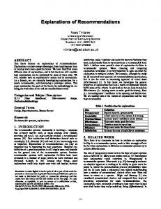
6.3. Shopping Simulation We recruited a convenience sample of 67 participants from an undergraduate business course. We encouraged participation by giving students the option of participating in the study or completing another task of equivalent time commitment to receive a three percent bonus on their course grade. These students took part in a laboratory study in small groups of 10 to 20. Each subject participated individually at a pre-configured computer. We told the participants that the study’s purpose was to improve our understanding of electronic commerce and online catalogs. After reviewing the study purpose and agreeing to take part, participants viewed the study directions online (Figure 3). The directions were embedded in the shopping simulation website such that participants could return to them at any time. In short, participants were asked to pretend that they were shopping, look at whatever they wanted to for however long they wanted to, and add items they wanted to “buy” to their shopping baskets.


496


Figure 3. Front Page of Simulated Catalog Participants then took part in a simulated shopping exercise. Participants could view as many or as few item pages as they chose for as little or as much time as they wished. Participants could return to a previously-viewed item page—of 3669 item page views in total, 428 (11.7%) were repeats. This low repeat rate is consistent with browsing (rather than searching) behavior. Item pages were generated from the datastore (training set) created during the pretests. Figure 4 depicts a sample item page. Item pages contained all of the italicized attributes indicated in Table 1, not just the attributes used by DESIRE. All item pages in each product category were as similar as possible, with exactly the same attributes listed and exactly one picture. The system recorded the time each participant spent viewing each item page. Participants could navigate among the available items either by browsing “departments”; that is, listings by product category (Figure 5) or by keyword search. Participants could add any number of items to their shopping basket, which could be viewed at any time. Looking at the shopping basket (Figure 6), participants could remove items, “proceed to checkout”, or continue shopping. Clicking the “proceed to checkout” button ended the simulation, consistent with the directions provided. This phase produced the data store of viewing time triples. Where a participant viewed the same item page repeatedly, total viewing time was used. No recommendations were generated or displayed during the shopping simulation.

497



Figure 4. Sample Item Page

Figure 5. Sample Product Listing by Category


498


Figure 6. Sample Shopping Cart

6.4. Explicit Item Rating After completing the shopping simulation, participants were asked to rate a series of items they had not previously seen (the holdout set, which was randomly selected from the set of all catalog items). Participants were shown an item page similar to the item pages in the shopping simulation but with a nine-point rating scale. Up to ten items were presented per product category; however, if a participant did not view any items from one or more categories in the shopping simulation, that participant was not asked to rate items from those categories. During this phase, an explicit ratings data store comprising 930 explicit product ratings was constructed. No recommendations were generated or displayed during the explicit item rating phase.

6.5. DESIRE Computation With data collection complete, the DESIRE algorithm (Appendix A) was run. Input data included the item data store (including attribute data), the relative attribute importance index, and the item viewing times from the shopping simulation (but not the explicit item rating page). This produced a set of estimated ratings for holdout-set items in each product category in which the participant had viewed items during the simulation. We could then compute DESIRE’s accuracy by comparing DESIRE’s estimated ratings of holdout items to users’ explicit ratings of the same holdout items.

7. Results and Discussion 7.1. Comparing DESIRE to RANDOM Ratings To test Hypothesis 1 (that DESIRE ratings are better than RANDOM ratings), we compared the MAE of DESIRE’s ratings (versus the user-generated ratings described above) by product category to the MAE of RANDOM ratings. Tables 3 and 4 contain the results of independent-sample t-tests comparing DESIRE’s ratings with ratings generated from a uniform distribution and the observed distribution (from the product rating phase), respectively. The analysis in Table 3 demonstrates that the difference between DESIRE ratings and random (uniform) ratings was highly significant across all five product categories (using a Bonferroni-adjusted significance level of 0.01), with DESIRE performing substantially better than a system that generates ratings randomly. In addition, the

499



effect size ranged from moderate to high in all categories except boots (the rightmost column of Table 3 lists the Cohen’s-d statistic for each category tested, where we interpret 0.8 as high, 0.5 as moderate, and 0.2 as low). Table 3. T-test Results of DESIRE versus RANDOM (Uniform Distribution) Recommendations Category

N

DESIRE MAE SD

UNIFORM MAE SD

t

p

Cohen’s d

Notebook computers

182

1.52

1.12

2.77

2.12

7.0442

3, set ri = 3 b. For each item rating such that ri < -3, set ri = -3 3. For each ri, set ri = ri /3 Discussion of variations: At least three variations on this method are possible. First, outliers may be deleted instead of limited to the closer boundary of the [-1,1] range. Second, viewing times can be transformed to fit or approximate any distribution (not just a normal distribution) as long as the range of the returned values is [-1,1]. Third, a more complex function of viewing time can be employed; for example, one that adjusts for the complexity of the item.

User Profile Generator Description: Given a set of item/rating pairs, generate a description of the user’s preferences in terms of the attributes of the items. This is computed differently for numeric attributes than categorical attributes. Preconditions: The sets of item ratings and item attributes must not be empty; the positive example threshold must be ≥ 0. Input: 1) A set of n seen items, I, 2) a rating for each item, 3) a set of attributes (e.g., color, price) for each item, 4) a set of values (e.g. red, $15), corresponding to the attributes, for each item, 5) the positive example threshold. Output: A user preference profile, consisting of ideal values of numeric attributes and inferred ratings of categorical (non-numeric) attributes. Algorithm: 1. Divide the attributes into two groups, numeric and categorical, as follows a. If the data associated with an attribute is not unique to the item (e.g., the ISBN of a book), and the attribute is nominal or ordinal, assign the attribute to the categorical attribute group

509



b. If the data associated with an attribute is interval or ratio, assign the attribute to the numeric attribute group 2. Calculate Ideal Values of Numeric Attributes a. For each item, i, if the rating of i ≥ ‘positive example threshold,’ add i to the set of positive examples. b. For each numeric attribute found in one or more positive examples, calculate its “ideal value,” as a weighted average of the attribute’s value in positive examples, as follows. Here, ri is the rating of the ith positive example, vai is the value of attribute a in the ith positive example and IVa is the ideal value of attribute a.

3. Calculate Ratings of Categorical Attributes For each value, v, of each categorical attribute of each item, calculate the rating of v as the mean rating of items having v. (e.g., if three items are red, the rating of red is the mean rating of those three items). 4. Return the User Profile, consisting of the ideal values of each numeric attribute and the ratings of each categorical attribute value.

Recommendation Engine Description: Predict ratings of unseen items based on the user profile and recommend items with high predicted ratings. Input: 1) the user profile, U, 2) the unseen-item data store, D, consisting of a set of unseen items and their attributes, 3) a list of “relative importance weights” that indicate the importance of each attribute in determining preference, and 4) the number of recommendations requested. Preconditions: 1) The user profile must be non-empty; 2) The unseen-item datastore must be nonempty; 3) the intersection of attributes in the user profile and attributes of unseen items must be nonempty; 4) the list of “relative importance weights” must contain an entry corresponding to each attribute in both the user profile and datastore; 5) The number of recommendations requested must not exceed the number of unseen items. Output: A set or recommended items Algorithm: 1. Standardize numeric data. For each numeric attribute in the intersection of U and D: a. Replace all values of that attribute in D with their z-scores. b. Replace the ideal value of that attribute in U with its z-scores. 2. Let R be an empty list of item similarity/pairs. 3. For each unseen item, iu:


510


a. Let S be a list of attribute/similarity pairs b. For each categorical attribute, a, in iu: i)

Let s be the similarity of the value to the user profile

ii)

Set s as follows, where n is the number of values of a and U(Vj) is the user profile rating of the jth value of a (i.e., if an item is red and white, average the rating of red and white from the user profile, then convert from a [-1,1] range to a [0,1] range).

iii) Add (a, s) to S c.

For each numeric attribute, a, in iu: i)

Let s be the similarity of the value to the user profile

ii)

Set s as follows, where Va is the value of a and Ua is the ideal value of a from the user profile (i.e., calculate dissimilarity as the absolute value of the difference between the ideal value and the actual value, then divide by six to convert to a [0,1] range, and subtract from one to get similarity).

iii) Add (a, s) to S d. Let Ri be the overall similarity between the user profile, U and unseen item, i. e. Let W be the subset of relative importance weights corresponding to, and in the same order as, the attributes in S. f.

Set Ri as follows, where W a is the relative importance of attribute a, and Sa is the similarity of i to U in terms of a.

g. Add (i, Ri) to R. 4. Let be the subset of R having the n items with highest similarity, where n is the number of recommendations desired. 5. Return

511

.



Discussion of variations: Many variations on this method are possible. First, numeric attributes could be fit to distributions other than the standard, normal distribution, as long as they can be transformed to a [0,1] range. Second, if items could have multiple values for a numeric attribute, one could apply the same averaging technique as used to account for multiple categorical values per attribute. Third, different techniques for accounting for multiple values per attribute could be used; for example, instead of averaging the similarity of different values, DESIRE could simply choose the highest or lowest similarity. Fourth, instead of returning a set number of recommendations, DESIRE could return all of items exceeding a given similarity threshold. Fifth, DESIRE can incorporate a forgetting function (i.e., ignoring viewing data beyond a certain age or giving additional weight to more recent viewing history) to account for changing preferences.


512


About the Authors Jeffrey PARSONS is University Research Professor and Professor of Information Systems in the Faculty of Business Administration at Memorial University of Newfoundland. He holds a Ph.D. in Information Systems from the University of British Columbia. His research interests include conceptual modeling, data management, business intelligence, and recommender systems; he is especially interested in classification issues in these and other domains. His research has been published in journals such as Nature, Management Science, MIS Quarterly, Information Systems Research, Journal of Management Information Systems, Communications of the ACM, ACM Transactions on Database Systems, and IEEE Transactions on Software Engineering. He has served in several editorial roles, both for journals and conferences. Paul RALPH is a Lecturer in Information Systems at Lancaster University. He holds a Ph.D. in Information Systems from The University of British Columbia. His research centers on the theoretical and empirical study of software engineering and information systems development including projects, processes, practices, tools and designer cognition, socialization, productivity, wellbeing and effectiveness. His research has been published by IEEE, ACM, AIS, Springer, and Elsevier. He has served in several editorial roles, both for journals and conferences.

513
