Artificial neural networks (ANN) are a powerful general purpose tool applied to ... representing network into the symbolic description known as Rule extraction.
Generating predicate rules from neural networks Richi Nayak Centre for Information Innovation Technology, Queensland University of Technology, Brisbane Qld 4001, Australia
Abstract. Artificial neural networks play an important role for pattern recognition tasks. However, due to poor comprehensibility of the learned network, and the inability to represent explanation structures, they are not considered sufficient for the general representation of knowledge. This paper details a methodology that represents the knowledge of a trained network in the form of restricted first-order logic rules, and subsequently allows user interaction by interfacing with a knowledge based reasoner.
1
Introduction
Artificial neural networks (ANN) are a powerful general purpose tool applied to classification, prediction and clustering tasks. A recognised drawback of neural networks is an absence of the capability to explain the decision process in a comprehensive form. This can be overcome by reformation of numerical weights representing network into the symbolic description known as Rule extraction. Previous researchers have successfully extract the learned knowledge in a propositional attribute-value language [1]. While this is sufficient for some applications, but for many applications the sheer number of propositional rules often makes their comprehension difficult. A means to generate fewer general rules that are equivalent of many more simple rules in propositional ground form is necessary. A further reason to use a predicate, rather than a propositional calculus, is the greater expressiveness of the former. Predicate rules allow learning of general rules as well as learning of internal relationships among variables. This paper presents an approach which extracts rules from a trained ANN using a propositional rule-extraction method. It further enhances the expressiveness of generated rules with the introduction of universally quantified variables, terms, and predicates, creating a knowledge base equivalent to the network.
2
The Methodology
Given a set of positive training examples E + , a set of negative examples E − and a hypothesis in the form of the trained neural network ANN, the task is to find the set of rules consisting of n-ary predicates and quantified variables KR such + − + − that: ANN ∪ KR |= e+ and ANN ∪ KR 6|= e− i , ∀ei ∈ E i , ∀ei ∈ E .
The methodology includes four phases:(1) Select and train an ANN until it reaches the minimum training and validation error; (2) Start pruning the ANN to remove redundant links and nodes, and retrain; (3) Generate the representation consisting of a type-hierarchy, facts and predicate rules; and (4) Interface the generated knowledge base with a knowledge base (KB) reasoner to provide user interface. 2.1
Phase 1: ANN training and Phase 2:Pruning
A feedforward neural networks is trained for the given problem. When the ANN learning process completes, a pruning algorithm is applied to remove redundant nodes and links in the trained ANNs. The remaining nodes and links are trained for a few epochs to adjust the weights. 2.2
Phase 3: Rule extraction
The next task is interpretation of the knowledge embedded in trained ANNs as symbolic rules. Following is the discussion of generalisation inference rules required to implicate specific to general relationship in this phase [5]: 1. θ-subsumption: A clause C θ-subsumes (¹) a clause D, if there exists a substitution θ such that Cθ ⊆ D. C is known as the least general generalisation (lgg) of D, and D is specialisation of C if C ¹ D and, for every other E such that Eθ ⊆ D, it is also the case that Eθ ⊆ C [6]. The definition is extendible to calculate the least general generalisation of a set of clauses. The clause C is the lgg of a set of clauses S if C is the generalisation of each clause in S, and also a least general generalisation. 2. Turning constants into variables: If a number of descriptions with different constants are observed for a predicate or a formula, these observations are generalised into a generic predicate or formula. E.g., if a unary predicate (p) holds for various constants a, b, ..l then the predicate p can be generalised to hold every value of a variable V with V being either of a, b, ..l. 3. Counting arguments: Constructive generalisation rules generate inductive assertions during learning that use descriptors, originally not present in the given examples. The CQ count quantified variables rule generates descriptors #V cond, representing the number of Vi that satisfy some condition cond, if a concept descriptor is in the form of ∃V1 , V2 , .., Vl · p(V1 , V2 , .., Vk ). The CA count arguments of a predicate rule generates new descriptors #V cond, by measuring the number of arguments in the predicate that satisfy some condition cond, if the descriptor is a predicate with several arguments, p(V1 , V2 , ..). [5] 4. Term-rewriting: This reformulation rule transforms compound terms in elementary terms. Let p be an n-ary predicate, whose first argument is a compound term consisting of t1 and t2 , and the n − 1 arguments are represented by a list A. The rules to perform such transformation are: p(t1 ∨ t2 , A) ↔ p(t1 , A) ∨ p(t2 , A) p(t1 ∧ t2 , A) ↔ p(t1 , A) ∧ p(t2 , A)
The generalisation algorithm The method of mapping predicate rules from propositional expressions, summarised in Figure 1, is an automatic bottom-up processing utilising Plotkin’s lgg concept [6]. This is defined as the task of finding a generalised rule set represented in the subset language of first-order logic such that KR + |= C1+ ∨ ... ∨ Cn+ and KR − |= C1− ∨ ... ∨ Cn− , where KR + and KR − are knowledge representations that cover all positive (Ci+ ) and negative (Ci− ) conjunctive expressions respectively.
1. Search for a DNF expression equivalent to the neural network. 2. Generate a single-depth type-hierarchy by input-space mapping, with attributes as concepts, and values as sub-concepts. 3. Perform a symbol mapping for predicates to convert each conjunctive expression into a ground fact (such as N odename#1 #2 , hidden1 1 or output1 2, or simply p 1, p 2, .., p n). 4. Utilise the fact definitions to create specific clauses (clauses with constants, C1 ,C2 ,..,Cn ). 5. For all specific clauses do 5.1 Search for any two compatible clauses C1 and C2 . Let C1 ≡ {l1 , .., lk } and C2 ≡ {m1 , .., mk } where each li , mi has same predicate and sign. 5.2 If such a pair C1 and C2 exists do 5.2.1 Determine a set of selections, S(C1 , C2 ) := {(l1 , m1 ), .., (lk , mk )} 5.2.2 Compute a new word symbol to hold the two k-ary predicates word1 := T emp(l1 , .., lk ), word2 := T emp(m1 , .., mk ) 5.2.3 let θ1 := ∅, θ2 := ∅, q1 := word1 and q2 := word2 5.2.4 While q1 6= q2 do • Search arguments of q1 and q2 • find t1 ∈ q1 and t2 ∈ q2 such that t1 and t2 are occurring at the same position in q1 and q2 and t1 6= t2 or one of them is a variable. • Replace t1 and t2 with a new variable X whenever they occur in the same position of q1 and q2 . • Let θ1 := θ1 ∪ {t1 /X}, θ2 := θ2 ∪ {t2 /X} 5.2.5 A rule with predicates and variables is generated (word1 = q1 σ1 , word2 = q2 σ2 ) 6. Return the knowledge representation consisting of rules in the subset language of first order logic, facts and a type-hierarchy. Fig. 1. The process to generate the formalism of predicate rules
In this representation, definitions of predicates and terms are same as those in first-order logic except that terms are function free. The explicit negation of predicates is allowed in describing the goal concepts to avoid ‘negation-byfailure’. A fact is an instantiated/ground predicate if all its predicate variables are constant. There is a single-depth type-hierarchy corresponding to input space of an ANN, in which attributes are concepts, and their values are sub-concepts.
During the process of converting conjunctive expressions into ground facts: (1) If a conjunctive expression contains only one value per attribute, it results in one fact; (2) If a conjunctive expression contains more that one value for an attribute, it results in multiple fact by transforming the expression according to ‘term-rewriting rule of generalisation’. Minimisation procedures such as (1) deletion of duplicated instances of facts, (2) replacing specific facts by more general ones and (3) deleting redundant entities in compatible facts-same predicate symbol and sign, are applied to remove the redundant facts or entities in facts. The fact definitions are utilised to express specific rules. These specific rules are now expressed as clauses (disjunction of literals) by applying the logical equivalence law, P ⇒ Q ≡ ¬P ∨ Q. Plotkin’s ‘θ-subsumption rule of generalisation’ [6]is utilised to compute the mapping of literals of specific clauses to general clauses. To compute the generalisation of two clauses, literals must represent each possible mapping between the two clauses. The mapping is done by forming a set of pairs of compatible literals (i.e. same predicate symbol and sign) from the two clauses (in the same way as is done for Plotkin’s concept of selection [6, 8]). The set of selections of two clauses C1 = {l1 , .., lk } and C2 = {m1 , .., mk } is defined as: S(C1 , C2 ) := {(li , mj )|∀li ∈ C1 ∧ mj ∈ C2 ∧ compatible}. For computing the least general generalisation (lgg) of two clauses, the lgg of two literals requires to be computed first, and then the lgg of two terms (function free). The lgg of two clauses C1 and C2 is defined as: lgg(C1 , C2 ) = lgg(S(C1 , C2 )) = lgg(T emp(l1 , .., lk ), T emp(m1 , .., mk )) lgg(l1 , m1 ) = p(lgg(t1 , s1 ), .., (tn , sn )) A substitution θ = {X/t1 , X/t2 } uniquely maps two terms to a variable X in compatible predicates by replacing all occurrences of t1 and t2 with the variable X, whenever they occur together in the same position. This ensures that θ is the proper substitution of t1 and t2 . The size of the set of selections of two clauses C1 , C2 can be at most i × j, where i is the number of literals in C1 and j is the number of literals in C2 . In general the resulting lgg of two clauses contains a maximum of i × j literals, many of which may be redundant and can be reduced by applying Plotkin’s equivalence property. The lgg of two incompatible literals is undefined [6]. If there is a rule (with constants) left alone in the original set that does not have a pair with which to generalise this rule, is not reduced and just mapped in the appropriate format. An example We use a simple example of Monk1 (consisting of six attributes and 432 patterns) to illustrate the rule generalisation process. The decision rule for membership of the target class (i.e. a monk) is: (1) Head shape = Body shape, or (2) Jacket color = red. After training and pruning of an ANN over this problem, the input space is: Head shape ∈ {round, square, octagon}, Body shape ∈ {round, square, octagon}, and Jacket color ∈ {red, not-red}. A rule-extraction algorithm is applied to extract the knowledge of the ANN in propositional rules form. The DNF (disjunctive normal form) expression representing the output node having high output is:
1. (Head shape = round ∧ Body shape = round) ∨ 2. (Head shape = square ∧ Body shape = square) ∨ 3. (Head shape = octagon ∧ Body shape = octagon) ∨ 4. (Jacket color = red) ∨ The extracted DNF expression indicating the low output for the output node is: 5. (Head shape = round ∧ Body shape = square) ∨ 6. (Head shape = round ∧ Body shape = octagon) ∨ 7. (Head shape = square ∧ Body shape = round) ∨ 8. (Head shape = square ∧ Body shape = octagon) ∨ 9. (Head shape = octagon ∧ Body shape = round) ∨ 10. (Head shape = octagon ∧ Body shape = square). Each conjunctive expression is expressed as a ground fact. The first three expressions having the same arguments are mapped to the same predicate symbol: monk1(round, round), monk1(square, square), and monk1(octagon,octagon). The fourth expression is inferred as monk2(red). Likewise expressions 5 to 10 indicating a different category (low output) are mapped to a new predicate symbol monk3 with their corresponding values. A concept definition -monk(Head shape, Body shape, Jacket color) or monk(X, Y, Z)- for the output node (the consequent of rules) is formed by collecting dependencies among attributes (associated within facts). The specific inference rules including the ground facts are: 1. monk(round, round, Z) ⇐ monk1(round, round) 2. monk(square, square, Z) ⇐ monk1(square, square) 3. monk(octagon,octagon, Z) ⇐ monk1(octagon,octagon) 4. monk(X, Y, red) ⇐ monk2(red) 5. ¬monk(round, square, Z) ⇐ monk3(round, square) 6. ¬monk(round, octagon, Z) ⇐ monk3(round, octagon) 7. ¬monk(square, round, Z) ⇐ monk3(square, round) 8. ¬monk(square, octagon, Z) ⇐ monk3(square, octagon) 9. ¬monk(octagon, round, Z) ⇐ monk3(octagon, round) 10. ¬monk(octagon, square, Z) ⇒ monk3(octagon, square) The algorithm discussed in Figure 1 iterates over the rules to find two compatible rules. Let us take the compatible rules 5 to 10 to show the process of finding a lgg rule. On applying the logical equivalence law, P ⇒ Q ≡ ¬P ∨ Q, the rules 5 & 6 are transformed into: 1. ¬monk3(round, square) ∨ ¬monk(round, square, Z) 2. ¬monk1(round,octagon) ∨ ¬monk(round,octagon, Z) A new word symbol Temp is utilised to form two k-ary predicates to hold the set of selections generated from rules 5 and 6. Considering two choices for each antecedent, the set of selections of two rules contains a maximum of 2n literals. These two clauses have two selections with consequent predicate. 1. Temp(¬monk3(round,square),¬monk(round,square,Z)) 2. Temp(¬monk3(round,octagon),¬monk(round,octagon,Z)) The θ-subsumption proceeds with the following steps:
1. Temp(¬monk3(round,Y),¬monk(round,Y,Z)) 2. Temp(¬monk3(round,Y),¬monk(round,Y,Z)) resulting in the inference rule: • ¬monk(round,Y,Z) ⇐ monk3(round,Y) with θ = [Y/square] or [Y/octagon] This lgg rule is further θ-subsumpted with the rest of the compatible rules 7,8,9,10, resulting in the following rule: ∀ X,Y,Z ¬monk(X,Y,Z) ⇐ monk3(X,Y) The algorithm also finds an inference rule out of three compatible rules 1, 2 & 3: ∀ X,Z monk(X,X,Z) ⇐ monk1(X,X) For rule 4, the algorithm does not find any other compatible rule. This rule will therefore be: ∀ X,Y,Z monk(X,Y,Z) ⇐ (Z == red) It can be observed that these generated rules are able to capture the true learning objective of the Monk1 problem domain i.e. the higher order proposition that (Head shape = Body shape) (rule 1 & 2) rather than yielding each propositional rule such as Head shape = round and Body shape= round etc. 2.3
Phase 4: User interaction
The generated knowledge base is interfaced with a KB reasoner that allows user interaction and enables greater explanatory capability. The inference process is activated when the internal knowledge base is operationally loaded and consultation begins. For example, if the query monk(square, square, not-red) is posed, the KB system initiates and executes the appropriate rules and returns the answer true with the explanation: • monk(square,square,not-red) ⇐ monk1(square, square)
3
Evaluation
The methodology is successfully tested on a number of synthetic data sets such as Monks, Mushroom, Voting, Moral reasoner, Cleveland heart and Breast cancer from UCI machine learning repository and real-world data sets such as remote sensing and Queensland Railway crossing safety. The results are compared with symbolic propositional learner C5 and symbolic predicate learner FOIL [7]. Tables 1 and 2 report the relative overall performance of predicate rulesets utilising different algorithms. The average performance is determined by separately measuring the performance on each data set, and then calculating the average performance across all data sets, for each rule set. Several neural network learning techniques such as cascade correlation (CC), BpTower (BT) and constrained error back propagation (CEBP) are utilised to build networks. This is to show the the applicability of predicate (or restricted first-order) ruleextraction to a variety of ANN architectures. The included results are after the application of pruning algorithm (P) to reduce the input space. The proposed rule extraction techniques LAP [4] and RulVI [3] are applied on the cascade and BpTower ANNs. The Rulex [2] technique is applied to extract rules from the trained CEBPNs. Table 1 shows that the accuracy of the generated predicate rules very much depends on the rule-extraction algorithm that has been employed to extract
Table 1. The relative average predictive accuracy of predicate rules over 10 data sets Predicate rules Accuracy (%) Accuracy (%) Fidelity (%) using Training Testing to the network PCC 98.28 95.05 99.04 LAP PBT 98.21 95.15 98.88 PCC 97.65 89.57 98.27 RuleVI PBT 97.59 84.71 96.87 Rulex CEBPN 96.41 89.51 93.23 C4.5 96.99 94.05 Foil 97.1 83.98 Table 2. The relative average comprehensibility of predicate rules over 10 data sets
PCC LAP PBT PCC RuleVI PBT Rulex CEBPN C4.5 Foil
No of Conjunctive expressions No of Predicate rules 64 28 63 21 39 18 48 24 4.6 4 10 8
the propositional expressions from the trained ANN. The expressiveness of the extracted propositional expressions is enhanced by introducing variables and predicates in rules without the loss of accuracy or of fidelity to the ANN solution. If the relevance of a particular input attribute depends on the values of other input attributes, then the generalisation algorithm is capable of showing that relationship in terms of variables (as in Monk1). Otherwise the generalisation algorithm simply translates the propositional rules into predicate form without significantly reducing the number of rules. The generalization accuracy (when moving from training to test data) of FOIL is worse than our system. The generalization accuracy even becomes worse when the data has noise. Our method performed (in terms of accuracy and comprehensibility) better than symbolic learners when small amount of data (less than 100 patterns) is available for training. When a large number of data is available for training, symbolic learners performed better. Our system preformed better than FOIL when the distribution of patterns among classes is uneven. The algorithmic complexity of this methodology depends upon the core algorithms used in different phases. The generalisation algorithm used in phase 3 requires O(l × m2 ), where l is the number of clauses according to the DNF expression equivalent to the trained ANN and m is the total number of attributes in the problem domain. However, application of the pruning algorithm in phase 2 significantly reduces the total number of attributes.
4
Conclusion
We presented a methodology which comprehensively understands the decision process of an ANN, and provides explanations to the user by interfacing the network’s output with a KB reasoner. The powerful advantage of ANNs, the ability to learn and generalise, is exploited to extract knowledge from a set of examples. Even though ANNs are only capable of encoding simple propositional data, with the addition of the inductive generalisation step, the knowledge represented by the trained ANN is transformed into a representation consisting of rules with predicates, facts and a type-hierarchy. The qualitative knowledge representation ideas of symbolic systems are combined with the distributed computational advantages of connectionist models. The logic required in representing the network is restricted to pattern matching for the unification of predicate arguments and does not contain functions. Despite this fact, the predicate formalism is appropriate for real-life problems as shown in experiments. The benefit in using such a logic to represent networks is that (1) knowledge can be interactively queried leading to an identification of newly acquired concepts, (2) an equivalent symbolic interpretation is derived describing the overall behaviour, and (3) a fewer number of rules are relatively easier to understand.
References 1. R. Andrews, J. Diederich, and A. Tickle. A survey and critique of techniques for extracting rules from trained artificial neural networks. Knowledge Based Systems, 8:373–389, 1995. 2. R. Andrews and S. Geva. Rule extraction from a constrained error back propagation mlp. In Proc. of 5th Australian Conference on Neural Networks, Brisbane, Australia, pages 9–12, 1994. 3. R. Hayward, C. Ho-Stuart, and J. Diederich. Neural networks as oracles for rule extraction. In Connectionist System for Knowledge Representation and Deduction, pages 105–116. Queensland University of Technology, Australia, 1997. 4. R. Hayward, A. Tickle, and J. Diederich. Extracting rules for grammar recognition from cascade-2 networks. In Connectionist, Statistical and Symbolic Approaches to Learning for Natural Language Proc., pages 48–60. Springer-Verlag, Berlin, 1996. 5. R. S. Michalski and R. L. Chilausky. Knowledge acquisition by encoding expert rules versus computer induction from examples-a case study involving soya-bean pathology. International Journal of Man-Machine Studies, 12:63–87, 1980. 6. D. G. Plotkin. A further note on inductive generalisation. In B. Meltzer and D. Michie, editors, Machine Intelligence 6, volume 6, pages 101–124. Edinburgh University Press, 1971. 7. J. R. Quinlan. Learning logical definitions from relations. Machine Learning, 5(3):239–266, 1990. 8. S. Wrobel. Inductive logic programming. In G. Brewka, editor, Principles of Knowledge Representation. CSLI Publications and FoLLI, 1996.