earlier â was applied to the NSL-KDD data set, and each came up with a set of feature, shown in table II. In addition to the FS techniques applied in this paper, ...
Proceedings of the 2013 Federated Conference on Computer Science and Information Systems pp. 769–774
Genetic Algorithm with Different Feature Selection Techniques for Anomaly Detectors Generation Amira Sayed A. Aziz1,∗ , Ahmad Taher Azar2,∗ , Mostafa A. Salama3,∗ Aboul Ella Hassanien4,∗ and Sanaa El-Ola Hanafy4 1 Universite Francaise d’Egypte (UFE), Cairo, Egypt 2 Faculty of Computers and Information, Benha University, Egypt 3 British University in Egypt (BUE), Cairo, Egypt 4 Faculty of Computers and Information, Cairo University, Egypt ∗ Scientific Research Group in Egypt (SRGE) http://www.egyptscience.net
Abstract—Intrusion detection systems have been around for quite some time, to protect systems from inside ad outside threats. Researchers and scientists are concerned on how to enhance the intrusion detection performance, to be able to deal with real-time attacks and detect them fast from quick response. One way to improve performance is to use minimal number of features to define a model in a way that it can be used to accurately discriminate normal from anomalous behaviour. Many feature selection techniques are out there to reduce feature sets or extract new features out of them. In this paper, we propose an anomaly detectors generation approach using genetic algorithm in conjunction with several features selection techniques, including principle components analysis, sequential floating, and correlation-based feature selection. A Genetic algorithm was applied with deterministic crowding niching technique, to generate a set of detectors from a single run. The results show that sequential-floating techniques with the genetic algorithm have the best results, compared to others tested, especially the sequential floating forward selection with detection accuracy 92.86% on the train set and 85.38% on the test set. Index Terms—Anomaly detectors generation, genetic algorithms, feature selection
I. I NTRODUCTION ITH the expanding and increasing use of networks, and accumulating number of internet users, network throughput has become massive and threats are more diverse and sophisticated. Network and information security are of high importance, and research is continuous in these fields to keep up with the development of attacks. Intrusion Detection is a major research area that aims to identify suspicious activities in a monitored system, from authorized and unauthorized users. An Intrusion Detection System (IDS) could be hostbased or network-based. In Network IDSs (NIDS), network administrators are not able to keep up with the increase in network attacks number and complexity, for both known and unknown attacks. So, there is an urgent and pressing need for replacing them by automated systems for constant monitoring and quick responses [1]. Machine Learning techniques are used to create rules for an IDS by enhancing the domain knowledge. They improve performance by helping to automate
W
c 2013, IEEE 978-1-4673-4471-5/$25.00
the knowledge acquisition process by using training data to find and exploit regularities. They learn how to estimate knowledge from the training data sets. Because one of the biggest challenges of IDS is the massive amount of data collected from the system, learning algorithms are used to discover models that are appropriate to classify normal and anomalous behaviors [2][3]. Different machine learning (ML) techniques are used in the development of anomaly intrusion detection. They could be pattern classifiers, single classifiers, hybrid classifiers, or ensemble classifiers. Such techniques include Support Vector Machine (SVM), Artificial Neural Networks (ANN), SelfOrganizing Maps (SOM), Decision Trees (DT), Genetic Algorithms (GA), and many others. In this paper, a genetic algorithm is used to generate detectors for an anomaly intrusion detection system. Some feature selection techniques are applied for feature reduction, before applying the GA. The paper is organized as follows: Section II gives a background for different components of the system. Section III introduces the proposed anomaly detectors generation algorithm. Section IV describes the experiment steps and the involved data sets. Section V shows the experiment result. Conclusions and future work are discussed in Section VI. II. BACKGROUND A. Anomaly Intrusion Detection Intrusion Detection Systems can be classified - based on methodology - into misuse-based and anomaly-based. Misusebased IDS builds a database of attacks signatures and use them to detect anomalies. It’s accurate and definitive concerning detecting unknown that do not match the stored patterns. This is where the anomaly-based IDS acts better. Anomaly IDS builds a model that represents the normal behaviour of a system and assume that deviations from such model are attacks or suspicious activity. So, it detect unknown attacks but it may have a high false alarm rate, based on its adjustments. A model in anomaly IDS can be statistical, knowledge-based, or machine learning. A learning technique could be embedded too, to update and adjust the normal model from time to time,
769
´ PROCEEDINGS OF THE FEDCSIS. KRAKOW, 2013
770
to represent the actual system behaviour that may change from time to time [4][5]. B. Feature Selection For each problem with some sample, there is a maximum number of features where performance degrades instead of improves – which is called the curse of dimensionality. An accurate mapping of lower-dimensional space of features is needed so no information is lost by discarding important and basic features. Two issues one should pay attention to while doing this: (1) How dimensionality can affect classification accuracy and (2) How dimensionality affects a classifier complexity. A feature is good when it is relevant but not redundant to the other relevant features. There are two techniques to follow for this: feature extraction and feature selection. Feature extraction algorithms tend to create a new subset of features by combining existing features. Feature selection (FS) algorithms tend to limit the features to only those which would improve a task performance. The FS [6][7][8] is an essential machine learning technique that is important and efficient in building classification systems. When used to reduce features, it results in lower computation costs and better classification performance. Feature selection algorithms are composed of three components: search algorithm, evaluation function, and performance function. The search algorithm could be: exponential – which is expensive to use as they have exponential complexity in number of features, sequential where it adds and subtracts features, so they have polynomial complexity; or randomized – where it require biases to yield small subsets, and they usually achieve high accuracies. An objective function is a function to evaluate the candidate features for feature selection. Based on evaluation criteria, FS techniques can be divided into filter methods and wrapper methods. Filters evaluate feature subsets by their information content, using distance measures, correlation measures...etc. Wrappers use a classifier for features subset evaluation by their predictive accuracy. Filter techniques discards feature upon their evaluation based on data general characteristics or using some kind of statistical analysis, without any learning mechanism involved. Wrapper techniques use a learning algorithm to find the features subset with the best performance. They are more expensive computation-based, and slower due to the repeating process, but they give more accurate results than filter techniques. This might be a drawback for high dimensional data but it could be defeated by using a fast learning algorithm. 1) Correlation-based Feature Selection: Correlation Feature Selection (CFS) is a heuristic approach that evaluates the worthiness of a features subset. So, based on correlation concept, a feature is considered good if it is highly correlated to the class but not to the other features [9]. So, a suitable measure of correlation between features needs to be defined in which it represents the important and highly effective features. A function that evaluates the best individual feature is: M= p
k ∗rfc k + k ∗ (k − 1) ∗ r f f
(1)
Where: M is the heuristic merit of a features subset S containing K features, r f c is the average feature-class correlation, and r f f is the average feature-feature inter-correlation. The numerator indicates how predictive a group of features are; and the denominator indicates how much redundancy there is among those features. 2) Sequential Floating Selection: Sequential-floating selection is a flexible extension of sequential forward and backward selection (SFS and SBS respectively), with backtracking capabilities [10][11]. Sequential selection methods find optimal group of features by applying step-optimal method where in each step the best/worst feature is always added/discarded. No additional steps are taken to evaluate the selected features in each iteration to refine the subset. An improvement to the methodology is to apply the plus l-take away r method, where additional forward/backward steps are applied after each iteration to correct the selection decision in order to find the optimal final subset of features. If l > r then is Sequentialfloating forward selection, if l < r then it is sequentialfloating backward selection [12]. Sequential-Floating Forward Selection (SFFS) basically starts with an empty set, then at each iteration it adds sequentially the next best feature. Then, it tests if it maximizes the objective function when combined with the features already selected – and this is how SFS works. In addition to that, after each forward step, SFFS performs a backward step that discards the worst feature of the subset after a new feature is added. The backward steps are performed as long as the objective function is increasing. In a similar manner but in an opposite direction, SequentialFloating Backward Selection (SFBS) starts with the full set of features, then it sequentially removes the feature that least reduces the objective function value. This is how the SBS works. So, SFBS performs forward steps after each backward step, as long as the objective function increases. 3) Principle Components Analysis: Principal Components Analysis (PCA) is a way to find and highlight similarities and differences between data by identifying the existing patterns [13][14]. PCA is based in the idea that most information about classes are within the directions with the largest variations. It works in terms of standardized linear projection that maximizes the variance in the projected space. It is a powerful tool in the case of high-dimensional data. It calculates the eigenvectors of the covariance matrix to find the independent axes of the data. The main problem with PCA is that it does not take into consideration the class label of the feature vector, hence it does not consider class separability. 4) Information Gain: Information Gain (IG) help us to determine which feature is most useful for classification, using its entropy value. Entropy indicates the information content of a feature or how much information it is giving us. The higher the entropy, the more the information content. IG value is calculated as: IG(T, a) = H(T ) − H(T |a)
(2)
where H is the information entropy, T is a training example, and a ia a variable value. This equation calculates the IG
AMIRA SAYED A. AZIZ ET AL.: GENETIC ALGORITHMS WITH DIFFERENT FEATURE SELECTION TECHNIQUE
that a training example T obtains from an observation that a random variable A takes some value a. IG in machine learning is used to define a sequence of attributes to investigate, which leads to the building of a decision tree. A decision tree can be constructed top-down using the IG by first beginning at the root node, and use the attribute with the highest IG as an ancestor node. Then child nodes are added for each possible value of that attribute. All examples are attached to suitable child nodes where the examples values are identical to the node’s attached value. If the all examples attached to a child node can be labelled with a unique class label, then this node is marked as a leaf and that classification is added to the node. These steps are repeated until all classifications are added to the child nodes [15][16][17]. 5) Rough Sets: Rough Set Theory (RST) [18][19] can be used to discover dependencies in data for features reduction, using the data alone without additional information required. RST results in the most informative feature set, which would be the most predictive of the class label. The concepts are used to define necessity of features, which is calculated by functions of lower and upper approximations. The measures of necessity are employed as heuristics to guide the feature selection process. An information table is defined for the objects and the attributes as a tuple: T = (U, A)
(3)
where U is a finite non-empty set of the primitive objects, and A is a finite non-empty set of the attributes. Each feature is associated with a set of its values V . The attribute set would be divided into 2 subsets C and D, which are the condition and decision subsets, respectively. If P is a subset of A, the in-discernibility relation is defined as: IND(P) = {(x, y) ∈ UxU : ∀a ∈ P, a(x) = a(y)}
(4)
where a(x) is a feature value a of object x. x and y are said to be in-discernible with respect to P, if (x, y) ∈ IND(P) C. Genetic Algorithms As mentioned before, ML techniques are used to create rules for the intrusion detection systems, and genetic algorithms is a common algorithm that is been used for such purpose. Genetic Algorithms (GA) are search algorithms inspired by evolution and natural selection, and they can be used to solve different and diverse types of problems. The algorithm starts with a group of individuals (chromosomes) called a population. Each chromosome is composed of a sequence of genes that would be bits, characters, or numbers. Reproduction is achieved using crossover (2 parents are used to produce 1 or children) and mutation (alteration of a gene or more). Each chromosome is evaluated using a fitness function, which defines which chromosomes are highly-fitted in the environment. The process is iterated for multiple times for a number of generations until optimal solution is reached. The reached solution could be a single individual or a group of individuals obtained by repeating the GA process for many runs [20][21].
771
D. Negative Selection Approach Negative Selection Approach (NSA) as an artificial immune system (AIS) technique that is based on the self/non-self discrimination. It first builds a database of normal profiles, and then trains the detectors on that profile to be able to detect anomalous behaviour (that is not normal), when they are later released in the system. The detectors do this discrimination process by being able to recognize normal patterns, then any pattern that is not recognized as normal is considered anomalous. For its similarity to the anomaly detection concept, NSA has been widely applied in different anomaly intrusion detection and fault detection systems in different areas. NSA is very common and easy to implement, and it gives very good results specially when it is combined with classification techniques. Detectors generated and used are simply rules, that define low and high limits, or specific values, of the features used for the intrusion detection [22][23]. III. T HE P ROPOSED A NOMALY D ETECTORS G ENERATION A PPROACH In this paper, a genetic algorithms is applied with deterministic crowding niching technique, to generate a set of detectors in a single run. The detectors are generated following the NSA concept – as mentioned before – using the self samples from the training set. The original algorithm was originally implemented in [24] using only real-valued features. Then it was applied in [25] using a predefined set of features of different data types. Equal-width binning is applied on the features values as a preprocessing step to first create homogeneity between features, and second to discretize the values so that there would be no extreme values in the experiment. The number of bins for each feature was defined using the following formula. k = max(1, 2 ∗ log l)
(5)
where l is the number of observed values. Then each value is replaced with the enclosing bin (the bin that includes this value). Algorithm 1 shows the detailed steps of the detectors generation approach. A set S of normal connections (self particles) is defined in the beginning, to start generating the detectors that will be able to match normal connections in the future. The self space S is filled with randomly selected individuals from the normal connections in the training set. An individual is composed of a set of values representing the selected features for the IDS. Going through the GA process, crossover and mutation are applied where crossover provides exploitation and mutation provides exploration. The final result is a set of detectors (individuals) with features values that most represent normal connections. The fitness of an individual is measured by calculating the matching percentage between an individual and the normal samples, as follows: a (6) f itness(x) = A
´ PROCEEDINGS OF THE FEDCSIS. KRAKOW, 2013
772
Algorithm 1 GADG 1: Fill S Space with normal individuals from training set. 2: Run equal-width binning algorithm on continuous features. 3: Initialize population by selecting random individuals from the space S. 4: for The specified number of generations do 5: for The size of the population do 6: Select two individuals (with uniform probability) as parent1 and parent2 . 7: Apply crossover to produce a new individual (child). 8: Apply mutation to child. 9: Calculate the distance between child and parent1 as d1 , and the distance between child and parent2 as d2 . 10: Calculate the fitness of child, parent1 , and parent2 as f , f1 , and f2 respectively. 11: if (d1 < d2 ) and ( f > f1 ) then 12: replace parent1 with child 13: else 14: if (d2 f2 ) then 15: Replace parent2 with child. 16: end if 17: end if 18: end for 19: end for 20: Extract the best (highly-fitted) individuals as your final solution.
TABLE I D ISTRIBUTIONS OF NSL-KDD RECORDS Total Records Train 20%
25192
Train All
125973
Test+
22544
q d(X,Y ) = (x1 − y1 )2 + (x2 − y2 )2 . . . (xn − yn )2
(7)
The Minkowski distance, which uses the p-norm dimension as the power value, between two individuals is calculated as: n
d(X,Y ) = ( ∑ (|xi − yi | p ))1/p
(8)
i=0
IV. E XPERIMENTAL RESULTS AND DISCUSSION A. Data Set The NSL-KDD [26] data set was used in the experiment, as it is more refined and less biased than the original KDD Cup99 data set [27]. In addition to that, it contains much less number of records, so the whole training and test sets can be used in the experiments. Table I shows the distributions of normal and attacks records in the NSL-KDD data set.
DoS
Probe
13449 53.39% 67343 53.46% 9711 43.08%
9234 2289 36.65% 9.09% 45927 11656 36.456% 9.25% 7458 2421 33.08% 10.74%
U2R
R2L
11 0.04% 52 0.04% 200 0.89%
209 0.83% 995 0.79% 2754 12.22%
B. Feature Selection Each one of the feature selection – that were mentioned earlier – was applied to the NSL-KDD data set, and each came up with a set of feature, shown in table II. In addition to the FS techniques applied in this paper, other two sets of features selected in [3][28] using Information Gain (IG) and Rough Set (RS) for degree of dependency respectively, were used. TABLE II S ELECTED F EATURES FS Technique CFS SFBS SFFS PCA IG RS
where a is the number of samples matching the individual by 100% , and A is the total number of normal samples. where a is the number of samples matching the individual, and A is the total number of normal samples. Both the Euclidean and Minkowski distance measures were tested in the GA – each in a separate trial – to calculate the distance between a child and a parent. The Euclidean distance is also used in the discrimination function to detect anomalies. The Euclidean distance between two individuals is calculated as follow:
Normal
Selected features 3, 4, 8, 12, 29, 33, 39 2, 3, 6, 29, 34, 35, 36, 37, 38, 39, 40, 41 1, 2, 3, 4, 6, 7, 10, 12, 17, 22, 23, 24, 25, 26, 27, 28, 29, 30, 31, 32, 33, 34, 35, 36, 40, 41 1, 2, 3, 4, 5, 6, 7, 8, 9, 11, 13, 14, 17, 18, 22, 27, 28, 29, 31, 32, 35, 37 1, 6, 12, 15, 16, 17, 18, 19, 31, 32, 37 3, 6, 12, 23, 25, 26, 29, 30, 33, 34, 35, 36, 37, 38, 39
The suggested approach was executed for each set of features, then the generated detectors were tested against the Train Set and the Test Set to investigate the detection accuracy and which set of features gave the best results. The values used for the algorithm parameters are shown in table III. TABLE III PARAMETERS VALUES Population size Number of generations Mutation rate Crossover rate p
200, 400, 600 200, 500, 1000, 2000 2/L, where L is the number of features 1.0 0.5
A mutation rate is a measure of the likeness that random elements of your chromosome (individual) will be mutated, which is dependent on the number of features in our experiment. A crossover rate defines the percentage of chromosomes used in reproduction, in this case all selected chromosomes are used. The p norm set for the Minkowski distance measurement is selected as a small value between 0.0 and 1.0 to detect similarity more than difference. V. R ESULTS AND D ISCUSSION The algorithm was applied twice for each features group, with the two previously mentioned distance measurements.
AMIRA SAYED A. AZIZ ET AL.: GENETIC ALGORITHMS WITH DIFFERENT FEATURE SELECTION TECHNIQUE
Then, the resulted groups of detectors were tested against the whole Train Set and the Test Set. The performance measurements used are accuracy, sensitivity, and specificity, and they are calculated as:
Accuracy =
TP+TN T P + FN + T N + FP
(9)
TP T P + FN
(10)
Sensitivity =
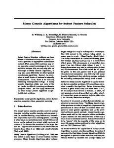
Fig. 2. Average Sensitivity for Train and Test Sets
Speci f icity =
TN T N + FP
(11)
Where: • • •
•
T P is the True Positives, when an attack is detected successfully and raises an alarm. T N is the True Negatives, when a normal connection does not raise an alarm. FP is the False Positives, when a normal connection is wrongfully detected as an attack and raises an alarm (false alarm). FN is the False Negatives, when an attack is not detected and does not raise an alarm.
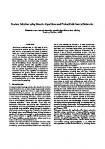
Accuracy mean how much accurate the system is to define anomalous and normal activities. Sensitivity expresses the ability of an IDS to correctly classify a connection as an attack. Specificity expresses the ability of an IDS to correctly classify a connection as normal. The average and maximum rates are shown in figures 10, 11, and 12 respectively.
Fig. 3. Average Specificity for Train and Test Sets
We can realize from the charts that CFS, SFFS, and PCA give the best results in general – figure 10. They give close results for the train set, but SFFS has the best results for the test set. Looking into the details, the SFFS selected features result in the best sensitivity rates (figure 11), which means the detectors can successfully detect anomalies in higher rates (91.87% and 92.15% for the train set, 89.7% and 90.21% for the test set). Although SFFS gives lower specificity rates (figure 12) than other algorithms, but as an overall no other algorithm resulted in such high true positive rates. We can realize too that although IG resulted in the highest specificity rates, it almost totally fails to classify anomalous activities in the data. VI. C ONCLUSION
Fig. 1. Average Accuracy for Train and Test Sets
In this paper, an anomaly-based, NSA inspired, network intrusion detection system was implemented, where GA was used to generate anomaly detectors for the system. In order to decide which features subset should be used, multiple feature selection approaches were used, and the results were compared to see which algorithm gave the best results. As shown above, although the SFFS gave the biggest features subset, it also gave the best accuracy and the best sensitivity rates - which is
773
´ PROCEEDINGS OF THE FEDCSIS. KRAKOW, 2013
774
most obvious on the Test set which includes unknown attacks. Checking the features selected by each algorithm, one can realize that: • Feature 3 — service — is very important in the detection process, it was not selected among the effective features using the IG technique and it shows poor performance in anomalies detection. • Feature 1 — duration – is also very important, it was selected by the techniques that resulted in better accuracy and detection rates. • Features that are concerned with the connection rates counts — 22, 29, 30, 31,...,41 — affects the performance too in a better way, they help improve detection accuracy. In the future, a classification technique should be used to classify the detected anomalies and refine the results more. R EFERENCES [1] J Bartlett, Machine Learning for Network Intrusion Detection, 2009. [2] Y Singh, P K Bhatia, O Sangwan, A review of studies on machine learning techniques, International Journal of Computer Science & Security, Vol. 1(1) , 2007, pp. 70-84. [3] HG Kayacik, AN Zincir-Heywood, MI Heywood, Selecting features for intrusion detection: a feature relevance analysis on KDD 99 intrusion detection data sets, Proceedings of the Third Annual Conference on Privacy, Security and Trust, October 2005. [4] P Garcia-Teodorro, J Diaz-Verdejo, G Marcia-Fernandez, E Vazquez, Anomaly-based network intrusion detection: Techniques, systems and challenges, Computers and Security, Elsevier, 2009, Vol. 28(1-2), pp. 18-28. [5] A Murali, M Roa, A survey on intrusion detection approaches, First International Conference on Information and Communication Technologies, ICICT 2005, IEEE. [6] P Langley, Selection of Relevant Features in Machine Learning, Defense Technical Information Center, 1994, pp. 140-144. [7] J Hua, WD Tembe, ER Dougherty, Performance of feature-selection methods in the classification of high-dimension data, Pattern Recognition, 2009, Vol. 42(3), pp. 409-424. [8] H Liu, H Motoda, L Yu, Feature selection with selective sampling, Machine Learning-International Workshop Then Conference, 2002, pp. 395-402. [9] L Yu and H Liu, Feature Selection for High-Dimensional Data – A Fast Correlation-Based Filter Solution, In Machine Learning-International Workshop Then Conference, 2003, Vol. 20(2), p. 856. [10] D W Aha and R L Bankert, A Comparative Evaluation of Sequential Feature Selection Algorithms, Learning from Data, 1996, pp. 199-206, Springer New York.
[11] R Gutierrez-Osuna, Pattern analysis for machine olfaction: a review, Sensors Journal, IEEE Vol. 2(3), 2002, pp. 189-202. [12] DW Aha and RL Bankert, A comparative evaluation of sequential feature selection algorithms, In Learning from Data, 1996, pp. 199206, Springer New York. [13] S Aksoy, Feature Reduction and Selection, Department of Computer Engineering Bilkent University, 2008, CS 551. [14] F Song, Z Guo, D Mei, Feature Selection Using Principal Component Analysis, System Science, Engineering Design and Manufacturing Informatization (ICSEM), 2010 International Conference on, Vol. 1, pp. 27-30 [15] M Hazewinkel, Information Encyclopedia of Mathematics, Springer, ISBN 978-1-55608-010-4, 2001. [16] DJC MacKay, Information theory, inference and learning algorithms, Cambridge university press, 2003. [17] D Roobaert, G Karakoulas, NV Chawla. Information gain, correlation and support vector machines. Feature Extraction, 2006, pp. 463-470, Springer Berlin Heidelberg. [18] M Zhang, and JT Yao, A rough sets based approach to feature selection, In Fuzzy Information, Processing NAFIPS’04. IEEE Annual Meeting of the, Vol. 1, 2004, pp. 434-439, IEEE. [19] R Jensen and Q Shen, Rough set based feature selection: A review, Rough Computing: Theories, Technologies and Applications, 2007. [20] W Li, Using Genetic Algorithm for Network Intrusion Detection, Proceedings of the United States Department of Energy Cyber Security Grou, Training Conference, 2004, Vol. 8, pp. 24-27. [21] C Sinclair, L Pierce, S Matzner, An Application of Machine Learning to Network Intrusion Detection, In Computer Security Applications Conference, ACSAC’99, Proceedings, 15th Annual, pp. 371-377, IEEE. [22] U Aickelin, J Greensmith, J Twycross , Immune system approaches to intrusion detection - a review, In Artificial Immune Systems, Springer Berlin Heidelberg, 2004, pp. 316-329. [23] D Dasgupta, Advances in artificial immune systems, IEEE Computational Intelligence Magazine, 2006, Vol. 1(4), pp. 409–49. [24] A S A Aziz, M A Salama, A E Hassanien, SE O Hanafi, Artificial Immune System Inspired Intrusion Detection System Using Genetic Algorithm. Informatica 36 (2012) 347-357 [25] A S A Aziz, A T Azar, A E Hassanien, SE O Hanafi,Continuous Features Discretizaion for Anomaly Intrusion Detectors Generation, 2012 Online Conference on Soft Computing in Industrial Applications Anywhere on Earth, 2012. [26] NSL-KDD Intrusion Detection data set, Available on: http://iscx.ca/NSL-KDD/, March 2009. [27] KDD Cup99 Intrusion Detection data set, Available on: http://kdd.ics.uci.edu/databases/kddcup99/kddcup99.html, October 2007. [28] A A Olusola, A S Oladele, D O Abosede, Analysis of KDD99 Intrusion Detection Dataset for Selection of Relevance Features, In Proceedings of the World Congress on Engineering and Computer Science, 2010, Vol. 1, pp. 20-22.