Genetic Algorithms

Introduction to Genetic Algorithms

S.N.Sivanandam · S.N.Deepa

Introduction to Genetic Algorithms

With 193 Figures and 13 Tables

Authors S.N.Sivanandam Professor and Head Dept. of Computer Science and Engineering PSG College of Technology Coimbatore - 641 004 TN, India

S.N.Deepa Ph.D Scholar Dept. of Computer Science and Engineering PSG College of Technology Coimbatore - 641 004 TN, India

Library of Congress Control Number: 2007930221

ISBN 978-3-540-73189-4 Springer Berlin Heidelberg New York This work is subject to copyright. All rights are reserved, whether the whole or part of the material is concerned, specifically the rights of translation, reprinting, reuse of illustrations, recitation, broadcasting, reproduction on microfilm or in any other way, and storage in data banks. Duplication of this publication or parts thereof is permitted only under the provisions of the German Copyright Law of September 9, 1965, in its current version, and permission for use must always be obtained from Springer. Violations are liable for prosecution under the German Copyright Law. Springer is a part of Springer Science+Business Media springer.com c Springer-Verlag Berlin Heidelberg 2008 The use of general descriptive names, registered names, trademarks, etc. in this publication does not imply, even in the absence of a specific statement, that such names are exempt from the relevant protective laws and regulations and therefore free for general use. Typesetting: Integra Software Services Pvt. Ltd., India Cover design: Erich Kirchner, Heidelberg Printed on acid-free paper

SPIN: 12053230

89/3180/Integra

5 4 3 2 1 0

Preface

The origin of evolutionary algorithms was an attempt to mimic some of the processes taking place in natural evolution. Although the details of biological evolution are not completely understood (even nowadays), there exist some points supported by strong experimental evidence: • Evolution is a process operating over chromosomes rather than over organisms. The former are organic tools encoding the structure of a living being, i.e., a creature is “built” decoding a set of chromosomes. • Natural selection is the mechanism that relates chromosomes with the efficiency of the entity they represent, thus allowing that efficient organism which is welladapted to the environment to reproduce more often than those which are not. • The evolutionary process takes place during the reproduction stage. There exists a large number of reproductive mechanisms in Nature. Most common ones are mutation (that causes the chromosomes of offspring to be different to those of the parents) and recombination (that combines the chromosomes of the parents to produce the offspring). Based upon the features above, the three mentioned models of evolutionary computing were independently (and almost simultaneously) developed. An Evolutionary Algorithm (EA) is an iterative and stochastic process that operates on a set of individuals (population). Each individual represents a potential solution to the problem being solved. This solution is obtained by means of a encoding/decoding mechanism. Initially, the population is randomly generated (perhaps with the help of a construction heuristic). Every individual in the population is assigned, by means of a fitness function, a measure of its goodness with respect to the problem under consideration. This value is the quantitative information the algorithm uses to guide the search. Among the evolutionary techniques, the genetic algorithms (GAs) are the most extended group of methods representing the application of evolutionary tools. They rely on the use of a selection, crossover and mutation operators. Replacement is usually by generations of new individuals. Intuitively a GA proceeds by creating successive generations of better and better individuals by applying very simple operations. The search is only guided by the fitness value associated to every individual in the population. This value is used to rank individuals depending on their relative suitability for the problem being v

vi

Preface

solved. The problem is the fitness function that for every individual is encharged of assigning the fitness value. The location of this kind of techniques with respect to other deterministic and non-deterministic procedures is shown in the following tree. This figure below outlines the situation of natural techniques among other well-known search procedures.

Combinations of EAs with Hill-Climbing algorithms are very powerful. Genetic algorithms intensively using such local search mechanism are termed Memetic Algorithms. Also parallel models increase the extension and quality of the search. The EAs exploration compares quite well against the rest of search techniques for a similar search effort. Exploitation is a more difficult goal in EAs but nowadays many solutions exist for EAs to refine solutions. Genetic algorithms are currently the most prominent and widely used computational models of evolution in artificial-life systems. These decentralized models provide a basis for understanding many other systems and phenomena in the world. Researches on GAs in alife give illustrative examples in which the genetic algorithm is used to study how learning and evolution interact, and to model ecosystems, immune system, cognitive systems, and social systems.

About the Book

This book is meant for a wide range of readers, who wishes to learn the basic concepts of Genetic Algorithms. It can also be meant for programmers, researchers and management experts whose work is based on optimization techniques. The basic concepts of Genetic Algorithms are dealt in detail with the relevant information and knowledge available for understanding the optimization process. The various operators involved for Genetic Algorithm operation are explained with examples. The advanced operators and the various classifications have been discussed in lucid manner, so that a starter can understand the concepts with a minimal effort. The solutions to specific problems are solved using MATLAB 7.0 and the solutions are given. The MATLAB GA toolbox has also been included for easy reference of the readers so that they can have hands on working with various GA functions. Apart from MATLAB solutions, certain problems are also solved using C and C++ and the solutions are given. The book is designed to give a broad in-depth knowledge on Genetic Algorithm. This book can be used as a handbook and a guide for students of all engineering disciplines, management sector, operational research area, computer applications, and for various professionals who work in Optimization area. Genetic Algorithms, at present, is a hot topic among academicians, researchers and program developers. Due to which, this book is not only for students, but also for a wide range of researchers and developers who work in this field. This book can be used as a ready reference guide for Genetic Algorithm research scholars. Most of the operators, classifications and applications for a wide variety of areas covered here fulfills as an advanced academic textbook. To conclude, we hope that the reader will find this book a helpful guide and a valuable source of information about Genetic Algorithm concepts for their several practical applications.

1 Organization of the Book The book contains 11 chapters altogether. It starts with the introduction to Evolutionary Computing. The various application case studies are also discussed. The chapters are organized as follows: vii

viii

About the Book

• Chapter 1 gives an introduction to Evolutionary computing, its development and its features. • Chapter 2 enhances the growth of Genetic Algorithms and its comparison with other conventional optimization techniques. Also the basic simple genetic algorithm with its advantages and limitations are discussed. • The various terminologies and the basic operators involved in genetic algorithm are dealt in Chap. 3. Few example problems, enabling the readers to understand the basic genetic algorithm operation are also included. • Chapter 4 discusses the advanced operators and techniques involved in genetic algorithm. • The different classifications of genetic algorithm are provided in Chap. 5. Each of the classifications is discussed with their operators and mode of operation to achieve optimized solution. • Chapter 6 gives a brief introduction to genetic programming. The steps involved and characteristics of genetic programming with its applications are described here. • Chapter 7 discusses on various genetic algorithm optimization problems which includes fuzzy optimization, multi objective optimization, combinatorial optimization, scheduling problems and so on. • The implementation of genetic algorithm using MATLAB is discussed in Chap. 8. The toolbox functions and simulated results to specific problems are provided in this chapter. • Chapter 9 gives the implementation of genetic algorithm concept using C and C++. The implementation is performed for few benchmark problems. • The application of genetic algorithm in various emerging fields along with case studies is given in Chapter 10. • Chapter 11 gives a brief introduction to particle swarm optimization and ant colony optimization. The Bibliography is given at the end for the ready reference of readers.

2 Salient Features of the Book The salient features of the book include: • • • • • • •

Detailed explanation of Genetic Algorithm concepts Numerous Genetic Algorithm Optimization Problems Study on various types of Genetic Algorithms Implementation of Optimization problem using C and C++ Simulated solutions for Genetic Algorithm problems using MATLAB 7.0 Brief description on the basics of Genetic Programming Application case studies on Genetic Algorithm on emerging fields

S.N. Sivanandam completed his B.E (Electrical and Electronics Engineering) in 1964 from Government College of Technology, Coimbatore and M.Sc (Engineering)

About the Book

ix

in Power System in 1966 from PSG College of Technology, Coimbatore. He acquired PhD in Control Systems in 1982 from Madras University. He has received Best Teacher Award in the year 2001 and Dhakshina Murthy Award for Teaching Excellence from PSG College of Technology. He received The CITATION for best teaching and technical contribution in the Year 2002, Government College of Technology, Coimbatore. He has a total teaching experience (UG and PG) of 41 years. The total number of undergraduate and postgraduate projects guided by him for both Computer Science and Engineering and Electrical and Electronics Engineering is around 600. He is currently working as a Professor and Head Computer Science and Engineering Department, PSG College of Technology, Coimbatore [from June 2000]. He has been identified as an outstanding person in the field of Computer Science and Engineering in MARQUIS “Who’s Who”, October 2003 issue, New providence, New Jersey, USA. He has also been identified as an outstanding person in the field of Computational Science and Engineering in “Who’s Who”, December 2005 issue, Saxe-Coburg Publications, United Kingdom. He has been placed as a VIP member in the continental WHO’s WHO Registry of national Business Leaders, Inc. 33 West Hawthorne Avenue Valley Stream, NY 11580, Aug 24, 2006. S.N. Sivanandam has published 12 books. He has delivered around 150 special lectures of different specialization in Summer/Winter school and also in various Engineering colleges. He has guided and coguided 30 Ph.D research works and at present 9 Ph.D research scholars are working under him. The total number of technical publications in International/National journals/Conferences is around 700. He has also received Certificate of Merit 2005–2006 for his paper from The Institution of Engineers (India). He has chaired 7 International conferences and 30 National conferences. He is a member of various professional bodies like IE (India), ISTE, CSI, ACS and SSI. He is a technical advisor for various reputed industries and Engineering Institutions. His research areas include Modeling and Simulation, Neural networks , Fuzzy Systems and Genetic Algorithm, Pattern Recognition, Multi dimensional system analysis, Linear and Non linear control system, Signal and Image processing, Control System, Power system, Numerical methods, Parallel Computing, Data Mining and Database Security. S.N. Deepa has completed her B.E Degree from Government College of Technology, Coimbatore, 1999 and M.E Degree from PSG College of Technology, Coimbatore, 2004. She was a gold medalist in her B.E Degree Programme. She has received G.D Memorial Award in the year 1997 and Best Outgoing Student Award from PSG College of Technology, 2004. Her M.E Thesis won National Award from the Indian Society of Technical Education and L&T, 2004. She has published 5 books and papers in International and National Journals. Her research areas include Neural Network, Fuzzy Logic, Genetic Algorithm, Digital Control, Adaptive and Non-linear Control.

Acknowledgement

The authors are always thankful to the Almighty for perseverance and achievements. They wish to thank Shri G. Rangaswamy, Managing Trustee, PSG Institutions, Shri C.R. Swaminathan, Chief Executive; and Dr. R. Rudramoorthy, Principal, PSG College of Technology, Coimbatore, for their whole-hearted cooperation and great encouragement given in this successful endeavor. They also wish to thank the staff members of computer science and engineering for their cooperation. Deepa wishes to thank her husband Anand, daughter Nivethitha and parents for their support.

xi

Contents

1 Evolutionary Computation . . . . . . . . . . . . . . . . . . . . . . . . . . . . . . . . . . . . . . . 1.1 Introduction . . . . . . . . . . . . . . . . . . . . . . . . . . . . . . . . . . . . . . . . . . . . . . . . . . 1.2 The Historical Development of EC . . . . . . . . . . . . . . . . . . . . . . . . . . . . . . . 1.2.1 Genetic Algorithms . . . . . . . . . . . . . . . . . . . . . . . . . . . . . . . . . . . . . . 1.2.2 Genetic Programming . . . . . . . . . . . . . . . . . . . . . . . . . . . . . . . . . . . . 1.2.3 Evolutionary Strategies . . . . . . . . . . . . . . . . . . . . . . . . . . . . . . . . . . 1.2.4 Evolutionary Programming . . . . . . . . . . . . . . . . . . . . . . . . . . . . . . . 1.3 Features of Evolutionary Computation . . . . . . . . . . . . . . . . . . . . . . . . . . . . 1.3.1 Particulate Genes and Population Genetics . . . . . . . . . . . . . . . . . . 1.3.2 The Adaptive Code Book . . . . . . . . . . . . . . . . . . . . . . . . . . . . . . . . . 1.3.3 The Genotype/Phenotype Dichotomy . . . . . . . . . . . . . . . . . . . . . . . 1.4 Advantages of Evolutionary Computation . . . . . . . . . . . . . . . . . . . . . . . . . 1.4.1 Conceptual Simplicity . . . . . . . . . . . . . . . . . . . . . . . . . . . . . . . . . . . 1.4.2 Broad Applicability . . . . . . . . . . . . . . . . . . . . . . . . . . . . . . . . . . . . . 1.4.3 Hybridization with Other Methods . . . . . . . . . . . . . . . . . . . . . . . . . 1.4.4 Parallelism . . . . . . . . . . . . . . . . . . . . . . . . . . . . . . . . . . . . . . . . . . . . . 1.4.5 Robust to Dynamic Changes . . . . . . . . . . . . . . . . . . . . . . . . . . . . . . 1.4.6 Solves Problems that have no Solutions . . . . . . . . . . . . . . . . . . . . . 1.5 Applications of Evolutionary Computation . . . . . . . . . . . . . . . . . . . . . . . . . 1.6 Summary . . . . . . . . . . . . . . . . . . . . . . . . . . . . . . . . . . . . . . . . . . . . . . . . . . . . .

1 1 2 2 3 4 5 5 6 7 8 9 10 10 11 11 11 12 12 13

2 Genetic Algorithms . . . . . . . . . . . . . . . . . . . . . . . . . . . . . . . . . . . . . . . . . . . . . . 2.1 Introduction . . . . . . . . . . . . . . . . . . . . . . . . . . . . . . . . . . . . . . . . . . . . . . . . . . 2.2 Biological Background . . . . . . . . . . . . . . . . . . . . . . . . . . . . . . . . . . . . . . . . . 2.2.1 The Cell . . . . . . . . . . . . . . . . . . . . . . . . . . . . . . . . . . . . . . . . . . . . . . . 2.2.2 Chromosomes . . . . . . . . . . . . . . . . . . . . . . . . . . . . . . . . . . . . . . . . . . 2.2.3 Genetics . . . . . . . . . . . . . . . . . . . . . . . . . . . . . . . . . . . . . . . . . . . . . . . 2.2.4 Reproduction . . . . . . . . . . . . . . . . . . . . . . . . . . . . . . . . . . . . . . . . . . . 2.2.5 Natural Selection . . . . . . . . . . . . . . . . . . . . . . . . . . . . . . . . . . . . . . . . 2.3 What is Genetic Algorithm? . . . . . . . . . . . . . . . . . . . . . . . . . . . . . . . . . . . . . 2.3.1 Search Space . . . . . . . . . . . . . . . . . . . . . . . . . . . . . . . . . . . . . . . . . . . 2.3.2 Genetic Algorithms World . . . . . . . . . . . . . . . . . . . . . . . . . . . . . . . . 2.3.3 Evolution and Optimization . . . . . . . . . . . . . . . . . . . . . . . . . . . . . . . 2.3.4 Evolution and Genetic Algorithms . . . . . . . . . . . . . . . . . . . . . . . . .

15 15 16 16 16 17 17 19 20 20 20 22 23

xiv

2.4

Contents

Conventional Optimization and Search Techniques . . . . . . . . . . . . . . . . . . 2.4.1 Gradient-Based Local Optimization Method . . . . . . . . . . . . . . . . . 2.4.2 Random Search . . . . . . . . . . . . . . . . . . . . . . . . . . . . . . . . . . . . . . . . . 2.4.3 Stochastic Hill Climbing . . . . . . . . . . . . . . . . . . . . . . . . . . . . . . . . . 2.4.4 Simulated Annealing . . . . . . . . . . . . . . . . . . . . . . . . . . . . . . . . . . . . 2.4.5 Symbolic Artificial Intelligence (AI) . . . . . . . . . . . . . . . . . . . . . . . A Simple Genetic Algorithm . . . . . . . . . . . . . . . . . . . . . . . . . . . . . . . . . . . . Comparison of Genetic Algorithm with Other Optimization Techniques . . . . . . . . . . . . . . . . . . . . . . . . . . . . . . . . . . . . . . . Advantages and Limitations of Genetic Algorithm . . . . . . . . . . . . . . . . . . Applications of Genetic Algorithm . . . . . . . . . . . . . . . . . . . . . . . . . . . . . . . Summary . . . . . . . . . . . . . . . . . . . . . . . . . . . . . . . . . . . . . . . . . . . . . . . . . . . . .

24 25 26 27 27 29 29

3 Terminologies and Operators of GA . . . . . . . . . . . . . . . . . . . . . . . . . . . . . . . 3.1 Introduction . . . . . . . . . . . . . . . . . . . . . . . . . . . . . . . . . . . . . . . . . . . . . . . . . . 3.2 Key Elements . . . . . . . . . . . . . . . . . . . . . . . . . . . . . . . . . . . . . . . . . . . . . . . . . 3.3 Individuals . . . . . . . . . . . . . . . . . . . . . . . . . . . . . . . . . . . . . . . . . . . . . . . . . . . 3.4 Genes . . . . . . . . . . . . . . . . . . . . . . . . . . . . . . . . . . . . . . . . . . . . . . . . . . . . . . . 3.5 Fitness . . . . . . . . . . . . . . . . . . . . . . . . . . . . . . . . . . . . . . . . . . . . . . . . . . . . . . . 3.6 Populations . . . . . . . . . . . . . . . . . . . . . . . . . . . . . . . . . . . . . . . . . . . . . . . . . . . 3.7 Data Structures . . . . . . . . . . . . . . . . . . . . . . . . . . . . . . . . . . . . . . . . . . . . . . . . 3.8 Search Strategies . . . . . . . . . . . . . . . . . . . . . . . . . . . . . . . . . . . . . . . . . . . . . . 3.9 Encoding . . . . . . . . . . . . . . . . . . . . . . . . . . . . . . . . . . . . . . . . . . . . . . . . . . . . . 3.9.1 Binary Encoding . . . . . . . . . . . . . . . . . . . . . . . . . . . . . . . . . . . . . . . . 3.9.2 Octal Encoding . . . . . . . . . . . . . . . . . . . . . . . . . . . . . . . . . . . . . . . . . 3.9.3 Hexadecimal Encoding . . . . . . . . . . . . . . . . . . . . . . . . . . . . . . . . . . . 3.9.4 Permutation Encoding (Real Number Coding) . . . . . . . . . . . . . . . 3.9.5 Value Encoding . . . . . . . . . . . . . . . . . . . . . . . . . . . . . . . . . . . . . . . . . 3.9.6 Tree Encoding . . . . . . . . . . . . . . . . . . . . . . . . . . . . . . . . . . . . . . . . . . 3.10 Breeding . . . . . . . . . . . . . . . . . . . . . . . . . . . . . . . . . . . . . . . . . . . . . . . . . . . . . 3.10.1 Selection . . . . . . . . . . . . . . . . . . . . . . . . . . . . . . . . . . . . . . . . . . . . . . 3.10.2 Crossover (Recombination) . . . . . . . . . . . . . . . . . . . . . . . . . . . . . . . 3.10.3 Mutation . . . . . . . . . . . . . . . . . . . . . . . . . . . . . . . . . . . . . . . . . . . . . . . 3.10.4 Replacement . . . . . . . . . . . . . . . . . . . . . . . . . . . . . . . . . . . . . . . . . . . 3.11 Search Termination (Convergence Criteria) . . . . . . . . . . . . . . . . . . . . . . . . 3.11.1 Best Individual . . . . . . . . . . . . . . . . . . . . . . . . . . . . . . . . . . . . . . . . . 3.11.2 Worst individual . . . . . . . . . . . . . . . . . . . . . . . . . . . . . . . . . . . . . . . . 3.11.3 Sum of Fitness . . . . . . . . . . . . . . . . . . . . . . . . . . . . . . . . . . . . . . . . . . 3.11.4 Median Fitness . . . . . . . . . . . . . . . . . . . . . . . . . . . . . . . . . . . . . . . . . 3.12 Why do Genetic Algorithms Work? . . . . . . . . . . . . . . . . . . . . . . . . . . . . . . . 3.12.1 Building Block Hypothesis . . . . . . . . . . . . . . . . . . . . . . . . . . . . . . . 3.12.2 A Macro-Mutation Hypothesis . . . . . . . . . . . . . . . . . . . . . . . . . . . . 3.12.3 An Adaptive Mutation Hypothesis . . . . . . . . . . . . . . . . . . . . . . . . . 3.12.4 The Schema Theorem . . . . . . . . . . . . . . . . . . . . . . . . . . . . . . . . . . . . 3.12.5 Optimal Allocation of Trials . . . . . . . . . . . . . . . . . . . . . . . . . . . . . .

39 39 39 39 40 41 41 42 43 43 43 44 44 44 45 45 46 46 50 56 57 59 59 60 60 60 60 61 62 62 63 65

2.5 2.6 2.7 2.8 2.9

33 34 35 36

Contents

3.13 3.14 3.15 3.16

3.17

3.18

3.12.6 Implicit Parallelism . . . . . . . . . . . . . . . . . . . . . . . . . . . . . . . . . . . . . . 3.12.7 The No Free Lunch Theorem . . . . . . . . . . . . . . . . . . . . . . . . . . . . . . Solution Evaluation . . . . . . . . . . . . . . . . . . . . . . . . . . . . . . . . . . . . . . . . . . . . Search Refinement . . . . . . . . . . . . . . . . . . . . . . . . . . . . . . . . . . . . . . . . . . . . . Constraints . . . . . . . . . . . . . . . . . . . . . . . . . . . . . . . . . . . . . . . . . . . . . . . . . . . Fitness Scaling . . . . . . . . . . . . . . . . . . . . . . . . . . . . . . . . . . . . . . . . . . . . . . . . 3.16.1 Linear Scaling . . . . . . . . . . . . . . . . . . . . . . . . . . . . . . . . . . . . . . . . . . 3.16.2 Sigma Truncation . . . . . . . . . . . . . . . . . . . . . . . . . . . . . . . . . . . . . . . 3.16.3 Power Law Scaling . . . . . . . . . . . . . . . . . . . . . . . . . . . . . . . . . . . . . . Example Problems . . . . . . . . . . . . . . . . . . . . . . . . . . . . . . . . . . . . . . . . . . . . . 3.17.1 Maximizing a Function . . . . . . . . . . . . . . . . . . . . . . . . . . . . . . . . . . 3.17.2 Traveling Salesman Problem . . . . . . . . . . . . . . . . . . . . . . . . . . . . . . Summary . . . . . . . . . . . . . . . . . . . . . . . . . . . . . . . . . . . . . . . . . . . . . . . . . . . . . Exercise Problems . . . . . . . . . . . . . . . . . . . . . . . . . . . . . . . . . . . . . . . . . . . . .

xv

66 68 68 69 69 70 70 71 72 72 72 76 78 81

4 Advanced Operators and Techniques in Genetic Algorithm . . . . . . . . . . 83 4.1 Introduction . . . . . . . . . . . . . . . . . . . . . . . . . . . . . . . . . . . . . . . . . . . . . . . . . . 83 4.2 Diploidy, Dominance and Abeyance . . . . . . . . . . . . . . . . . . . . . . . . . . . . . . 83 4.3 Multiploid . . . . . . . . . . . . . . . . . . . . . . . . . . . . . . . . . . . . . . . . . . . . . . . . . . . . 85 4.4 Inversion and Reordering . . . . . . . . . . . . . . . . . . . . . . . . . . . . . . . . . . . . . . . 86 4.4.1 Partially Matched Crossover (PMX) . . . . . . . . . . . . . . . . . . . . . . . . 88 4.4.2 Order Crossover (OX) . . . . . . . . . . . . . . . . . . . . . . . . . . . . . . . . . . . 88 4.4.3 Cycle Crossover (CX) . . . . . . . . . . . . . . . . . . . . . . . . . . . . . . . . . . . 89 4.5 Niche and Speciation . . . . . . . . . . . . . . . . . . . . . . . . . . . . . . . . . . . . . . . . . . . 89 4.5.1 Niche and Speciation in Multimodal Problems . . . . . . . . . . . . . . . 90 4.5.2 Niche and Speciation in Unimodal Problems . . . . . . . . . . . . . . . . . 93 4.5.3 Restricted Mating . . . . . . . . . . . . . . . . . . . . . . . . . . . . . . . . . . . . . . . 96 4.6 Few Micro-operators . . . . . . . . . . . . . . . . . . . . . . . . . . . . . . . . . . . . . . . . . . . 97 4.6.1 Segregation and Translocation . . . . . . . . . . . . . . . . . . . . . . . . . . . . . 97 4.6.2 Duplication and Deletion . . . . . . . . . . . . . . . . . . . . . . . . . . . . . . . . . 97 4.6.3 Sexual Determination . . . . . . . . . . . . . . . . . . . . . . . . . . . . . . . . . . . . 98 4.7 Non-binary Representation . . . . . . . . . . . . . . . . . . . . . . . . . . . . . . . . . . . . . . 98 4.8 Multi-Objective Optimization . . . . . . . . . . . . . . . . . . . . . . . . . . . . . . . . . . . . 99 4.9 Combinatorial Optimizations . . . . . . . . . . . . . . . . . . . . . . . . . . . . . . . . . . . . 100 4.10 Knowledge Based Techniques . . . . . . . . . . . . . . . . . . . . . . . . . . . . . . . . . . . 100 4.11 Summary . . . . . . . . . . . . . . . . . . . . . . . . . . . . . . . . . . . . . . . . . . . . . . . . . . . . . 102 Exercise Problems . . . . . . . . . . . . . . . . . . . . . . . . . . . . . . . . . . . . . . . . . . . . . 103 5 Classification of Genetic Algorithm . . . . . . . . . . . . . . . . . . . . . . . . . . . . . . . . 105 5.1 Introduction . . . . . . . . . . . . . . . . . . . . . . . . . . . . . . . . . . . . . . . . . . . . . . . . . . 105 5.2 Simple Genetic Algorithm (SGA) . . . . . . . . . . . . . . . . . . . . . . . . . . . . . . . . 105 5.3 Parallel and Distributed Genetic Algorithm (PGA and DGA) . . . . . . . . . 106 5.3.1 Master-Slave Parallelization . . . . . . . . . . . . . . . . . . . . . . . . . . . . . . 109 5.3.2 Fine Grained Parallel GAs (Cellular GAs) . . . . . . . . . . . . . . . . . . . 110 5.3.3 Multiple-Deme Parallel GAs (Distributed GAs or Coarse Grained GAs) . . . . . . . . . . . . . . . . . . . . . . . . . . . . . . . . . . . . . . . . . . 111

xvi

5.4

5.5

5.6 5.7

5.8

Contents

5.3.4 Hierarchical Parallel Algorithms . . . . . . . . . . . . . . . . . . . . . . . . . . . 113 Hybrid Genetic Algorithm (HGA) . . . . . . . . . . . . . . . . . . . . . . . . . . . . . . . . 115 5.4.1 Crossover . . . . . . . . . . . . . . . . . . . . . . . . . . . . . . . . . . . . . . . . . . . . . . 116 5.4.2 Initialization Heuristics . . . . . . . . . . . . . . . . . . . . . . . . . . . . . . . . . . 117 5.4.3 The RemoveSharp Algorithm . . . . . . . . . . . . . . . . . . . . . . . . . . . . . 117 5.4.4 The LocalOpt Algorithm . . . . . . . . . . . . . . . . . . . . . . . . . . . . . . . . . 119 Adaptive Genetic Algorithm (AGA) . . . . . . . . . . . . . . . . . . . . . . . . . . . . . . 119 5.5.1 Initialization . . . . . . . . . . . . . . . . . . . . . . . . . . . . . . . . . . . . . . . . . . . . 120 5.5.2 Evaluation Function . . . . . . . . . . . . . . . . . . . . . . . . . . . . . . . . . . . . . 120 5.5.3 Selection operator . . . . . . . . . . . . . . . . . . . . . . . . . . . . . . . . . . . . . . . 121 5.5.4 Crossover operator . . . . . . . . . . . . . . . . . . . . . . . . . . . . . . . . . . . . . . 121 5.5.5 Mutation operator . . . . . . . . . . . . . . . . . . . . . . . . . . . . . . . . . . . . . . . 122 Fast Messy Genetic Algorithm (FmGA) . . . . . . . . . . . . . . . . . . . . . . . . . . . 122 5.6.1 Competitive Template (CT) Generation . . . . . . . . . . . . . . . . . . . . . 123 Independent Sampling Genetic Algorithm (ISGA) . . . . . . . . . . . . . . . . . . 124 5.7.1 Independent Sampling Phase . . . . . . . . . . . . . . . . . . . . . . . . . . . . . . 125 5.7.2 Breeding Phase . . . . . . . . . . . . . . . . . . . . . . . . . . . . . . . . . . . . . . . . . 126 Summary . . . . . . . . . . . . . . . . . . . . . . . . . . . . . . . . . . . . . . . . . . . . . . . . . . . . . 127 Exercise Problems . . . . . . . . . . . . . . . . . . . . . . . . . . . . . . . . . . . . . . . . . . . . . 129

6 Genetic Programming . . . . . . . . . . . . . . . . . . . . . . . . . . . . . . . . . . . . . . . . . . . 131 6.1 Introduction . . . . . . . . . . . . . . . . . . . . . . . . . . . . . . . . . . . . . . . . . . . . . . . . . . 131 6.2 Comparison of GP with Other Approaches . . . . . . . . . . . . . . . . . . . . . . . . . 131 6.3 Primitives of Genetic Programming . . . . . . . . . . . . . . . . . . . . . . . . . . . . . . . 135 6.3.1 Genetic Operators . . . . . . . . . . . . . . . . . . . . . . . . . . . . . . . . . . . . . . . 136 6.3.2 Generational Genetic Programming . . . . . . . . . . . . . . . . . . . . . . . . 136 6.3.3 Tree Based Genetic Programming . . . . . . . . . . . . . . . . . . . . . . . . . . 136 6.3.4 Representation of Genetic Programming . . . . . . . . . . . . . . . . . . . . 137 6.4 Attributes in Genetic Programming . . . . . . . . . . . . . . . . . . . . . . . . . . . . . . . 141 6.5 Steps of Genetic Programming . . . . . . . . . . . . . . . . . . . . . . . . . . . . . . . . . . . 143 6.5.1 Preparatory Steps of Genetic Programming . . . . . . . . . . . . . . . . . . 143 6.5.2 Executional Steps of Genetic Programming . . . . . . . . . . . . . . . . . . 146 6.6 Characteristics of Genetic Programming . . . . . . . . . . . . . . . . . . . . . . . . . . . 149 6.6.1 What We Mean by “Human-Competitive” . . . . . . . . . . . . . . . . . . . 149 6.6.2 What We Mean by “High-Return” . . . . . . . . . . . . . . . . . . . . . . . . . 152 6.6.3 What We Mean by “Routine” . . . . . . . . . . . . . . . . . . . . . . . . . . . . . 154 6.6.4 What We Mean by “Machine Intelligence” . . . . . . . . . . . . . . . . . . 154 6.7 Applications of Genetic Programming . . . . . . . . . . . . . . . . . . . . . . . . . . . . 156 6.7.1 Applications of Genetic Programming in Civil Engineering . . . . . . . . . . . . . . . . . . . . . . . . . . . . . . . . . . . . . 156 6.8 Haploid Genetic Programming with Dominance . . . . . . . . . . . . . . . . . . . . 159 6.8.1 Single-Node Dominance Crossover . . . . . . . . . . . . . . . . . . . . . . . . 161 6.8.2 Sub-Tree Dominance Crossover . . . . . . . . . . . . . . . . . . . . . . . . . . . 161 6.9 Summary . . . . . . . . . . . . . . . . . . . . . . . . . . . . . . . . . . . . . . . . . . . . . . . . . . . . . 161 Exercise Problems . . . . . . . . . . . . . . . . . . . . . . . . . . . . . . . . . . . . . . . . . . . . . 163

Contents

xvii

7 Genetic Algorithm Optimization Problems . . . . . . . . . . . . . . . . . . . . . . . . . 165 7.1 Introduction . . . . . . . . . . . . . . . . . . . . . . . . . . . . . . . . . . . . . . . . . . . . . . . . . . 165 7.2 Fuzzy Optimization Problems . . . . . . . . . . . . . . . . . . . . . . . . . . . . . . . . . . . 165 7.2.1 Fuzzy Multiobjective Optimization . . . . . . . . . . . . . . . . . . . . . . . . . 166 7.2.2 Interactive Fuzzy Optimization Method . . . . . . . . . . . . . . . . . . . . . 168 7.2.3 Genetic Fuzzy Systems . . . . . . . . . . . . . . . . . . . . . . . . . . . . . . . . . . 168 7.3 Multiobjective Reliability Design Problem . . . . . . . . . . . . . . . . . . . . . . . . . 170 7.3.1 Network Reliability Design . . . . . . . . . . . . . . . . . . . . . . . . . . . . . . . 170 7.3.2 Bicriteria Reliability Design . . . . . . . . . . . . . . . . . . . . . . . . . . . . . . 174 7.4 Combinatorial Optimization Problem . . . . . . . . . . . . . . . . . . . . . . . . . . . . . 176 7.4.1 Linear Integer Model . . . . . . . . . . . . . . . . . . . . . . . . . . . . . . . . . . . . 178 7.4.2 Applications of Combinatorial Optimization . . . . . . . . . . . . . . . . . 179 7.4.3 Methods . . . . . . . . . . . . . . . . . . . . . . . . . . . . . . . . . . . . . . . . . . . . . . . 182 7.5 Scheduling Problems . . . . . . . . . . . . . . . . . . . . . . . . . . . . . . . . . . . . . . . . . . . 187 7.5.1 Genetic Algorithm for Job Shop Scheduling Problems (JSSP) . . 187 7.6 Transportation Problems . . . . . . . . . . . . . . . . . . . . . . . . . . . . . . . . . . . . . . . . 190 7.6.1 Genetic Algorithm in Solving Transportation Location-Allocation Problems with Euclidean Distances . . . . . . . 191 7.6.2 Real-Coded Genetic Algorithm (RCGA) for Integer Linear Programming in Production-Transportation Problems with Flexible Transportation Cost . . . . . . . . . . . . . . . . . . . . . . . . . . 194 7.7 Network Design and Routing Problems . . . . . . . . . . . . . . . . . . . . . . . . . . . 199 7.7.1 Planning of Passive Optical Networks . . . . . . . . . . . . . . . . . . . . . . 199 7.7.2 Planning of Packet Switched Networks . . . . . . . . . . . . . . . . . . . . . 202 7.7.3 Optimal Topological Design of All Terminal Networks . . . . . . . . 203 7.8 Summary . . . . . . . . . . . . . . . . . . . . . . . . . . . . . . . . . . . . . . . . . . . . . . . . . . . . . 208 Exercise Problems . . . . . . . . . . . . . . . . . . . . . . . . . . . . . . . . . . . . . . . . . . . . . 209 8 Genetic Algorithm Implementation Using Matlab . . . . . . . . . . . . . . . . . . . 211 8.1 Introduction . . . . . . . . . . . . . . . . . . . . . . . . . . . . . . . . . . . . . . . . . . . . . . . . . . 211 8.2 Data Structures . . . . . . . . . . . . . . . . . . . . . . . . . . . . . . . . . . . . . . . . . . . . . . . . 211 8.2.1 Chromosomes . . . . . . . . . . . . . . . . . . . . . . . . . . . . . . . . . . . . . . . . . . 212 8.2.2 Phenotypes . . . . . . . . . . . . . . . . . . . . . . . . . . . . . . . . . . . . . . . . . . . . . 212 8.2.3 Objective Function Values . . . . . . . . . . . . . . . . . . . . . . . . . . . . . . . . 213 8.2.4 Fitness Values . . . . . . . . . . . . . . . . . . . . . . . . . . . . . . . . . . . . . . . . . . 213 8.2.5 Multiple Subpopulations . . . . . . . . . . . . . . . . . . . . . . . . . . . . . . . . . 213 8.3 Toolbox Functions . . . . . . . . . . . . . . . . . . . . . . . . . . . . . . . . . . . . . . . . . . . . . 214 8.4 Genetic Algorithm Graphical User Interface Toolbox . . . . . . . . . . . . . . . . 219 8.5 Solved Problems using MATLAB . . . . . . . . . . . . . . . . . . . . . . . . . . . . . . . . 224 8.6 Summary . . . . . . . . . . . . . . . . . . . . . . . . . . . . . . . . . . . . . . . . . . . . . . . . . . . . . 260 Review Questions . . . . . . . . . . . . . . . . . . . . . . . . . . . . . . . . . . . . . . . . . . . . . 261 Exercise Problems . . . . . . . . . . . . . . . . . . . . . . . . . . . . . . . . . . . . . . . . . . . . . 261 9 Genetic Algorithm Optimization in C/C++ . . . . . . . . . . . . . . . . . . . . . . . . . 263 9.1 Introduction . . . . . . . . . . . . . . . . . . . . . . . . . . . . . . . . . . . . . . . . . . . . . . . . . . 263 9.2 Traveling Salesman Problem (TSP) . . . . . . . . . . . . . . . . . . . . . . . . . . . . . . . 263

xviii

9.3 9.4 9.5 9.6 9.7 9.8 9.9

Contents

Word Matching Problem . . . . . . . . . . . . . . . . . . . . . . . . . . . . . . . . . . . . . . . . 271 Prisoner’s Dilemma . . . . . . . . . . . . . . . . . . . . . . . . . . . . . . . . . . . . . . . . . . . . 280 Maximize f(x) = x2 . . . . . . . . . . . . . . . . . . . . . . . . . . . . . . . . . . . . . . . . . . . . 286 Minimization a Sine Function with Constraints . . . . . . . . . . . . . . . . . . . . . 292 9.6.1 Problem Description . . . . . . . . . . . . . . . . . . . . . . . . . . . . . . . . . . . . . 293 Maximizing the Function f(x) = x∗ sin(10∗ Π ∗ x) + 10 . . . . . . . . . . . . . . . 302 Quadratic Equation Solving . . . . . . . . . . . . . . . . . . . . . . . . . . . . . . . . . . . . . 310 Summary . . . . . . . . . . . . . . . . . . . . . . . . . . . . . . . . . . . . . . . . . . . . . . . . . . . . . 315 9.9.1 Projects . . . . . . . . . . . . . . . . . . . . . . . . . . . . . . . . . . . . . . . . . . . . . . . . 315

10 Applications of Genetic Algorithms . . . . . . . . . . . . . . . . . . . . . . . . . . . . . . 317 10.1 Introduction . . . . . . . . . . . . . . . . . . . . . . . . . . . . . . . . . . . . . . . . . . . . . . . . . . 317 10.2 Mechanical Sector . . . . . . . . . . . . . . . . . . . . . . . . . . . . . . . . . . . . . . . . . . . . . 317 10.2.1 Optimizing Cyclic-Steam Oil Production with Genetic Algorithms . . . . . . . . . . . . . . . . . . . . . . . . . . . . . . . . . 317 10.2.2 Genetic Programming and Genetic Algorithms for Auto-tuning Mobile Robot Motion Control . . . . . . . . . . . . . . . 320 10.3 Electrical Engineering . . . . . . . . . . . . . . . . . . . . . . . . . . . . . . . . . . . . . . . . . . 324 10.3.1 Genetic Algorithms in Network Synthesis . . . . . . . . . . . . . . . . . . . 324 10.3.2 Genetic Algorithm Tools for Control Systems Engineering . . . . . 328 10.3.3 Genetic Algorithm Based Fuzzy Controller for Speed Control of Brushless DC Motor . . . . . . . . . . . . . . . . . . . . . . . . . . . . . . . . . . . 334 10.4 Machine Learning . . . . . . . . . . . . . . . . . . . . . . . . . . . . . . . . . . . . . . . . . . . . . 341 10.4.1 Feature Selection in Machine learning using GA . . . . . . . . . . . . . 341 10.5 Civil Engineering . . . . . . . . . . . . . . . . . . . . . . . . . . . . . . . . . . . . . . . . . . . . . . 345 10.5.1 Genetic Algorithm as Automatic Structural Design Tool . . . . . . . 345 10.5.2 Genetic Algorithm for Solving Site Layout Problem . . . . . . . . . . 350 10.6 Image Processing . . . . . . . . . . . . . . . . . . . . . . . . . . . . . . . . . . . . . . . . . . . . . . 352 10.6.1 Designing Texture Filters with Genetic Algorithms . . . . . . . . . . . 352 10.6.2 Genetic Algorithm Based Knowledge Acquisition on Image Processing . . . . . . . . . . . . . . . . . . . . . . . . . . . . . . . . . . . . . 357 10.6.3 Object Localization in Images Using Genetic Algorithm . . . . . . . 362 10.6.4 Problem Description . . . . . . . . . . . . . . . . . . . . . . . . . . . . . . . . . . . . . 363 10.6.5 Image Preprocessing . . . . . . . . . . . . . . . . . . . . . . . . . . . . . . . . . . . . . 364 10.6.6 The Proposed Genetic Algorithm Approach . . . . . . . . . . . . . . . . . 365 10.7 Data Mining . . . . . . . . . . . . . . . . . . . . . . . . . . . . . . . . . . . . . . . . . . . . . . . . . . 367 10.7.1 A Genetic Algorithm for Feature Selection in Data-Mining . . . . 367 10.7.2 Genetic Algorithm Based Fuzzy Data Mining to Intrusion Detection . . . . . . . . . . . . . . . . . . . . . . . . . . . . . . . . . . . . 370 10.7.3 Selection and Partitioning of Attributes in Large-Scale Data Mining Problems Using Genetic Algorithm . . . . . . . . . . . . . . . . . 379 10.8 Wireless Networks . . . . . . . . . . . . . . . . . . . . . . . . . . . . . . . . . . . . . . . . . . . . . 386 10.8.1 Genetic Algorithms for Topology Planning in Wireless Networks . . . . . . . . . . . . . . . . . . . . . . . . . . . . . . . . . . . . 386 10.8.2 Genetic Algorithm for Wireless ATM Network . . . . . . . . . . . . . . . 387 10.9 Very Large Scale Integration (VLSI) . . . . . . . . . . . . . . . . . . . . . . . . . . . . . . 395

Contents

xix

10.9.1 Development of a Genetic Algorithm Technique for VLSI Testing . . . . . . . . . . . . . . . . . . . . . . . . . . . . . . . . . . . . . . . . 395 10.9.2 VLSI Macro Cell Layout Using Hybrid GA . . . . . . . . . . . . . . . . . 397 10.9.3 Problem Description . . . . . . . . . . . . . . . . . . . . . . . . . . . . . . . . . . . . . 398 10.9.4 Genetic Layout Optimization . . . . . . . . . . . . . . . . . . . . . . . . . . . . . . 399 10.10 Summary . . . . . . . . . . . . . . . . . . . . . . . . . . . . . . . . . . . . . . . . . . . . . . . . . . . . . 402 11 Introduction to Particle Swarm Optimization and Ant Colony Optimization . . . . . . . . . . . . . . . . . . . . . . . . . . . . . . . . . . . . . . . . . . . . . . . . . . . 403 11.1 Introduction . . . . . . . . . . . . . . . . . . . . . . . . . . . . . . . . . . . . . . . . . . . . . . . . . . 403 11.2 Particle Swarm Optimization . . . . . . . . . . . . . . . . . . . . . . . . . . . . . . . . . . . . 403 11.2.1 Background of Particle Swarm Optimization . . . . . . . . . . . . . . . . 404 11.2.2 Operation of Particle Swarm Optimization . . . . . . . . . . . . . . . . . . 405 11.2.3 Basic Flow of Particle Swarm Optimization . . . . . . . . . . . . . . . . . 407 11.2.4 Comparison Between PSO and GA . . . . . . . . . . . . . . . . . . . . . . . . 408 11.2.5 Applications of PSO . . . . . . . . . . . . . . . . . . . . . . . . . . . . . . . . . . . . . 410 11.3 Ant Colony Optimization . . . . . . . . . . . . . . . . . . . . . . . . . . . . . . . . . . . . . . . 410 11.3.1 Biological Inspiration . . . . . . . . . . . . . . . . . . . . . . . . . . . . . . . . . . . . 410 11.3.2 Similarities and Differences Between Real Ants and Artificial Ants . . . . . . . . . . . . . . . . . . . . . . . . . . . . . . . . . . . . . . . 414 11.3.3 Characteristics of Ant Colony Optimization . . . . . . . . . . . . . . . . . 415 11.3.4 Ant Colony Optimization Algorithms . . . . . . . . . . . . . . . . . . . . . . . 416 11.3.5 Applications of Ant Colony Optimization . . . . . . . . . . . . . . . . . . . 422 11.4 Summary . . . . . . . . . . . . . . . . . . . . . . . . . . . . . . . . . . . . . . . . . . . . . . . . . . . . . 424 Exercise Problems . . . . . . . . . . . . . . . . . . . . . . . . . . . . . . . . . . . . . . . . . . . . . 424 Bibliography . . . . . . . . . . . . . . . . . . . . . . . . . . . . . . . . . . . . . . . . . . . . . . . . . . . . . . . 425

Chapter 1

Evolutionary Computation

1.1 Introduction Charles Darwinian evolution in 1859 is intrinsically a so bust search and optimization mechanism. Darwin’s principle “Survival of the fittest” captured the popular imagination. This principle can be used as a starting point in introducing evolutionary computation. Evolved biota demonstrates optimized complex behavior at each level: the cell, the organ, the individual and the population. Biological species have solved the problems of chaos, chance, nonlinear interactivities and temporality. These problems proved to be in equivalence with the classic methods of optimization. The evolutionary concept can be applied to problems where heuristic solutions are not present or which leads to unsatisfactory results. As a result, evolutionary algorithms are of recent interest, particularly for practical problems solving. The theory of natural selection proposes that the plants and animals that exist today are the result of millions of years of adaptation to the demands of the environment. At any given time, a number of different organisms may co-exist and compete for the same resources in an ecosystem. The organisms that are most capable of acquiring resources and successfully procreating are the ones whose descendants will tend to be numerous in the future. Organisms that are less capable, for whatever reason, will tend to have few or no descendants in the future. The former are said to be more fit than the latter, and the distinguishing characteristics that caused the former to be fit are said to be selected for over the characteristics of the latter. Over time, the entire population of the ecosystem is said to evolve to contain organisms that, on average, are more fit than those of previous generations of the population because they exhibit more of those characteristics that tend to promote survival. Evolutionary computation (EC) techniques abstract these evolutionary principles into algorithms that may be used to search for optimal solutions to a problem. In a search algorithm, a number of possible solutions to a problem are available and the task is to find the best solution possible in a fixed amount of time. For a search space with only a small number of possible solutions, all the solutions can be examined in a reasonable amount of time and the optimal one found. This exhaustive search, however, quickly becomes impractical as the search space grows in size. Traditional search algorithms randomly sample (e.g., random walk) or heuristically sample (e.g., gradient descent) the search space one solution at a time in the hopes 1

2

1 Evolutionary Computation

of finding the optimal solution. The key aspect distinguishing an evolutionary search algorithm from such traditional algorithms is that it is population-based. Through the adaptation of successive generations of a large number of individuals, an evolutionary algorithm performs an efficient directed search. Evolutionary search is generally better than random search and is not susceptible to the hill-climbing behaviors of gradient-based search. Evolutionary computing began by lifting ideas from biological evolutionary theory into computer science, and continues to look toward new biological research findings for inspiration. However, an over enthusiastic “biology envy” can only be to the detriment of both disciplines by masking the broader potential for two-way intellectual traffic of shared insights and analogizing from one another. Three fundamental features of biological evolution illustrate the range of potential intellectual flow between the two communities: particulate genes carry some subtle consequences for biological evolution that have not yet translated mainstream EC; the adaptive properties of the genetic code illustrate how both communities can contribute to a common understanding of appropriate evolutionary abstractions; finally, EC exploration of representational language seems pre-adapted to help biologists understand why life evolved a dichotomy of genotype and phenotype.

1.2 The Historical Development of EC In the case of evolutionary computation, there are four historical paradigms that have served as the basis for much of the activity of the field: genetic algorithms (Holland, 1975), genetic programming (Koza, 1992, 1994), evolutionary strategies (Recheuberg, 1973), and evolutionary programming (Forgel et al., 1966). The basic differences between the paradigms lie in the nature of the representation schemes, the reproduction operators and selection methods.

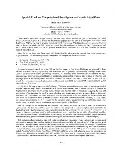
1.2.1 Genetic Algorithms The most popular technique in evolutionary computation research has been the genetic algorithm. In the traditional genetic algorithm, the representation used is a fixed-length bit string. Each position in the string is assumed to represent a particular feature of an individual, and the value stored in that position represents how that feature is expressed in the solution. Usually, the string is “evaluated as a collection of structural features of a solution that have little or no interactions”. The analogy may be drawn directly to genes in biological organisms. Each gene represents an entity that is structurally independent of other genes. The main reproduction operator used is bit-string crossover, in which two strings are used as parents and new individuals are formed by swapping a sub-sequence between the two strings (see Fig. 1.1). Another popular operator is bit-flipping mutation, in which a single bit in the string is flipped to form a new offspring string

1.2 The Historical Development of EC

3

Fig. 1.1 Bit-string crossover of parents a & b to form offspring c & d

(see Fig. 1.2). A variety of other operators have also been developed, but are used less frequently (e.g., inversion, in which a subsequence in the bit string is reversed). A primary distinction that may be made between the various operators is whether or not they introduce any new information into the population. Crossover, for example, does not while mutation does. All operators are also constrained to manipulate the string in a manner consistent with the structural interpretation of genes. For example, two genes at the same location on two strings may be swapped between parents, but not combined based on their values. Traditionally, individuals are selected to be parents probabilistically based upon their fitness values, and the offspring that are created replace the parents. For example, if N parents are selected, then N offspring are generated which replace the parents in the next generation.

1.2.2 Genetic Programming An increasingly popular technique is that of genetic programming. In a standard genetic program, the representation used is a variable-sized tree of functions and values. Each leaf in the tree is a label from an available set of value labels. Each internal node in the tree is label from an available set of function labels. The entire tree corresponds to a single function that may be evaluated. Typically, the tree is evaluated in a leftmost depth-first manner. A leaf is evaluated as the corresponding value. A function is evaluated using arguments that is the result of the evaluation of its children. Genetic algorithms and genetic programming are similar in most other respects, except that the reproduction operators are tailored to a tree representation. The most commonly used operator is subtree crossover, in which an entire subtree is swapped between two parents (see Fig. 1.3). In a standard genetic program, all values and functions are assumed to return the same type, although functions may vary in the number of arguments they take. This closure principle (Koza, 1994) allows any subtree to be considered structurally on par with any other subtree, and ensures that operators such as sub-tree crossover will always produce legal offspring.

Fig. 1.2 Bit-flipping mutation of parent a to form offspring b

4


Fig. 1.3 Subtree crossover of parents a & b to form offspring c & d

1.2.3 Evolutionary Strategies In evolutionary strategies, the representation used is a fixed-length real-valued vector. As with the bitstrings of genetic algorithms, each position in the vector corresponds to a feature of the individual. However, the features are considered to be behavioral rather than structural. “Consequently, arbitrary non-linear interactions between features during evaluation are expected which forces a more holistic approach to evolving solutions” (Angeline, 1996). The main reproduction operator in evolutionary strategies is Gaussian mutation, in which a random value from a Gaussian distribution is added to each element of an individual’s vector to create a new offspring (see Fig. 1.4). Another operator that is used is intermediate recombination, in which the vectors of two parents are averaged together, element by element, to form a new offspring (see Fig. 1.5). The effects of these operators reflect the behavioral as opposed to structural interpretation of the representation since knowledge of the values of vector elements is used to derive new vector elements. The selection of parents to form offspring is less constrained than it is in genetic algorithms and genetic programming. For instance, due to the nature of the representation, it is easy to average vectors from many individuals to form a single offspring. In a typical evolutionary strategy, N parents are selected uniformly randomly

Fig. 1.4 Gaussian mutation of parent a to form offspring b

1.3 Features of Evolutionary Computation

5

Fig. 1.5 Intermediate recombination of parents a & b to form offspring c

(i.e., not based upon fitness), more than N offspring are generated through the use of recombination, and then N survivors are selected deterministically. The survivors are chosen either from the best N offspring (i.e., no parents survive) or from the best N parents and offspring.

1.2.4 Evolutionary Programming Evolutionary programming took the idea of representing individuals’ phenotypic ally as finite state machines capable of responding to environmental stimuli and developing operators for effecting structural and behavioral change over time. This idea was applied to a wide range of problems including prediction problems, optimization and machine learning. The above characterizations, leads one to the following observations. GA practitioners are seldom constrained to fixed-length binary implementations. GP enables the use of variable sized tree of functions and values. ES practitioners have incorporated recombination operators into their systems. EP is used for the evolution of finite state machines. The representations used in evolutionary programming are typically tailored to the problem domain. One representation commonly used is a fixed-length realvalued vector. The primary difference between evolutionary programming and the previous approaches is that no exchange of material between individuals in the population is made. Thus, only mutation operators are used. For real-valued vector representations, evolutionary programming is very similar to evolutionary strategies without recombination. A typical selection method is to select all the individuals in the population to be the N parents, to mutate each parent to form N offspring, and to probabilistically select, based upon fitness, N survivors from the total 2N individuals to form the next generation.

1.3 Features of Evolutionary Computation In an evolutionary algorithm, a representation scheme is chosen by the researcher to define the set of solutions that form the search space for the algorithm. A number of individual solutions are created to form an initial population. The following steps are then repeated iteratively until a solution has been found which satisfies a pre-defined termination criterion. Each individual is evaluated using a fitness function that is specific to the problem being solved. Based upon their fitness values,

6


a number of individuals are chosen to be parents. New individuals, or offspring, are produced from those parents using reproduction operators. The fitness values of those offspring are determined. Finally, survivors are selected from the old population and the offspring to form the new population of the next generation. The mechanisms determining which and how many parents to select, how many offspring to create, and which individuals will survive into the next generation together represent a selection method. Many different selection methods have been proposed in the literature, and they vary in complexity. Typically, though, most selection methods ensure that the population of each generation is the same size. EC techniques continue to grow in complexity and desirability, as biological research continues to change our perception of the evolutionary process. In this context, we introduce three fundamental features of biological evolution: 1. particulate genes and population genetics 2. the adaptive genetic code 3. the dichotomy of genotype and phenotype Each phenomenon is chosen to represent a different point in the spectrum of possible relationships between computing and biological evolutionary theory. The first is chosen to ask whether current EC has fully transferred the basics of biological evolution. The second demonstrates how both biological and computational evolutionary theorists can contribute to common understanding of evolutionary abstractions. The third is chosen to illustrate a question of biological evolution that EC seems better suited to tackle than biology.

1.3.1 Particulate Genes and Population Genetics Mainstream thinking of the time viewed the genetic essence of phenotype as a liquid that blended whenever male and female met to reproduce. It took the world’s first professor of engineering, Fleming Jenkin (1867), to point out the mathematical consequence of blending inheritance: a novel advantageous mutation arising in a sexually reproducing organism would dilute itself out of existence during the early stages of its spread through any population comprising more than a few individuals. This is a simple consequence of biparental inheritance. Mendels’ theory of particulate genes (Mendel, 1866) replaced this flawed, analogue concept of blending inheritance with a digital system in which the advantageous version (allele) of a gene is either present or absent and biparental inheritance produces diploidy. Thus natural selection merely alters the proportions of alleles in a population, and an advantageous mutation can be selected into fixation (presence within 100% of individuals) without any loss in its fitness. Though much has been written about the Neo-Darwinian Synthesis that ensured from combining Mendelian genetics with Darwinian theory, it largely amounts to biologists’ gradual acceptance that the particulate nature of genes alone provided a solid foundation to build detailed, quantitative predictions about evolution.

1.3 Features of Evolutionary Computation

7

Indeed, decision of mathematical models of genes in populations as “bean bag genetics” overlooks the scope of logical deductions that follow from particulate genetics. They extend far beyond testable explanations for adaptive phenomena and into deeper, abstract concepts of biological evolution. For example, particulate genes introduce stochasticity into evolution. Because genes are either present or absent from any given genome, the genetic makeup of each new individual in a sexually reproducing population is a probabilistic outcome of which particular alleles it inherits from each parent. Unless offspring are infinite in number, their allele frequencies will not accurately mirror those of the parental generation, but instead will show some sampling error (genetic drift). The magnitude of this sampling error is inversely proportional to the size of a population. Wright (1932) noted that because real populations fluctuate in size, temporary reductions can briefly relax selection, potentially allowing gene pools to diffuse far enough away from local optima to find new destinations when population size recovers and selection reasserts itself. In effect, particulate genes in finite populations improve the evolutionary heuristic from a simple hill climbing algorithm to something closer to simulated annealing under a fluctuating temperature. One final property of particulate genes operating in sexual populations is worthy of mention. In the large populations where natural selection works most effectively, any novel advantageous mutation that arises will only reach fixation over the course of multiple generations. During this spread, recombination and diploidy together ensure that the allele will temporarily find itself in many different genetic contexts. Classical population genetics (e.g., Fisher, 1930) and experimental EC systems (e.g., O’Reilly, 1999) have focused on whether and how this context promotes selective pressure for gene linkage into “co-adapted gene complexes”. A simpler observation is that a novel, advantageous allele’s potential for negative epistatic effects is integral to its micro-evolutionary success. Probability will favor the fixation of alleles that are good “team players” (i.e., reliably imbue their advantage regardless of genetic background. Many mainstream EC methods simplify the population genetics of new mutations (e.g., into tournaments), to expedite the adaptive process. This preserves non-blending inheritance and even genetic drift, but it is not clear that it incorporates population genetics’ implicit filter for “prima donna” alleles that only offer their adaptive advantage when their genetic context is just so. Does this basic difference between biology and EC contribute anything to our understanding of why recombination seems to play such different roles in the two systems?

1.3.2 The Adaptive Code Book Molecular biology’s Central Dogma connects genes to phenotype by stating that DNA is transcribed into RNA, which is then translated into protein. The terms transcription and translation are quite literal: RNA is a chemical sister language to DNA. Both are polymers formed from an alphabet of four chemical letters (nucleotides), and transcription is nothing more than a process of complementing DNA, letter by letter, into RNA. It is the next step, translation

8


that profoundly influences biological evolution. Proteins are also linear polymers of chemical letters, but they are drawn from a qualitatively different alphabet (amino acids) comprising 20 elements. Clearly no one-to-one mapping could produce a genetic code for translating nucleotides unambiguously into amino acids, and by 1966 it was known that the combinatorial set of possible nucleotide triplets forms a dictionary of “codons” that each translate into a single amino acid meaning. The initial surprise for evolutionary theory was to discover that something as fundamental as the code-book for life would exhibit a high degree of redundancy (an alphabet of 4 RNA letters permits 4×4×4 = 64 possible codons that map to one of only 20 amino acid meanings). Early interpretation fuelled arguments for Non-Darwinian evolution: genetic variations that make no difference to the protein they encode must be invisible to selection and therefore governed solely by drift. More recently, both computing and biological evolutionary theory have started to place this coding neutrality in the bigger picture of the adaptive heuristic. Essentially, findings appear to mirror Wright’s early arguments on the importance of genetic drift: redundancy in the code adds selectively neutral dimensions to the fitness landscape that renders adaptive algorithms more effective by increasing the connectedness of local optima. At present, an analogous reinterpretation is underway for a different adaptive feature of the genetic code: the observation that biochemically similar amino acids are assigned to codons that differ by only a single nucleotide. Early speculations that natural selection organized the genetic code so as to minimize the phenotypic impact of mutations have gained considerable evidential support as computer simulation enables exploration of theoretical codes that nature passed over. However, it seems likely that once again this phenomenon has more subtle effects in the broader context of the adaptive heuristic. An “error minimizing code” may in fact maximize the probability that a random effects on both traits defines a circle of radius around the organism. The probability that this mutation will improve fitness (i.e., that the organism will move within the white area) is inversely proportional to its magnitude, mutation produces an increase in fitness according to Geometric Theory of gradualism (Fig. 1.6). Preliminary tests for this phenomenon reveal an even simpler influence: the error minimizing code smoothes the fitness landscape where a random genetic code would render it rugged. By clustering biochemically similar amino acids within mutational reach of one another it ensures that any selection towards a specific amino acid property (e.g., hydrophobicity) will be towards an interconnected region of the fitness landscape rather than to an isolated local optimum.

1.3.3 The Genotype/Phenotype Dichotomy Implicit to the concept of an adaptive genetic code is a deeper question that remains largely unanswered by biology: why does all known life use two qualitatively different polymers, nucleic acids and proteins, with the associated need for translation? Current theories for the origin of this dichotomy focus on the discovery that RNA can act both as a genetic storage medium, and as a catalytic molecule. Within the

1.4 Advantages of Evolutionary Computation

9

Fig. 1.6 The fitness landscape for an organism of 2 phenotypic traits: (a) for any organism, we may define an isocline that connects all trait combinations of equal fitness; (b) (the fitness landscape from above): a random mutation of magnitude that has tradeoff

most highly conserved core of metabolism, all known organisms are found to use RNA molecules in roles we normally attribute to proteins (White, 1976). However, the answer to how the dichotomy evolved has largely eclipsed the question of why RNA evolved a qualitatively different representation for phenotype. A typical biological answer would be that the larger alphabet size of amino acids unleashed a greater catalytic diversity for the replicators, with an associated increase in metabolic sophistication that optimized self-replication. Interestingly, we know that nucleic acids are not limited to the 4 chemical letters we see today: natural metabolically active RNA’s utilize a vast repertoire of posttranscriptional modifications and synthetic chemistry has demonstrated that multiple additional nucleotide letters can be added to the genetic alphabet even with today’s cellular machinery. Furthermore, an increasing body of indirect evidence suggests that the protein alphabet itself underwent exactly the sort of evolutionary expansion early in life’s history. Given the ubiquity of nucleic acid genotype and protein phenotype within life, biology is hard-pressed to assess the significance of evolving this “representational language”. The choice of phrase is deliberate: clearly the EC community is far ahead of biology in formalizing the concept of representational language, and exploring what it means. Biology will gain when evolutionary programmers place our system within their findings, illustrating the potential for biological inspiration from EC.

1.4 Advantages of Evolutionary Computation Evolutionary computation, describes the field of investigation that concerns all evolutionary algorithms and offers practical advantages to several optimization problems. The advantages include the simplicity of the approach, its robust response to changing circumstances, and its flexibility and so on. This section briefs some of

10


these advantages and offers suggestions in designing evolutionary algorithms for real-world problem solving.

1.4.1 Conceptual Simplicity A key advantage of evolutionary computation is that it is conceptually simple. Figure 1.7 shows a flowchart of an evolutionary algorithm applied for function optimization. The algorithm consists of initialization, iterative variation and selection in light of a performance index. In particular, no gradient information needs to be presented to the algorithm. Over iterations of random variation and selection, the population can be made to converge to optimal solutions. The effectiveness of an evolutionary algorithm depends on the variation and selection operators as applied to a chosen representation and initialization.

1.4.2 Broad Applicability Evolutionary algorithms can be applied to any problems that can be formulated as function optimization problems. To solve these problems, it requires a data structure to represent solutions, to evaluate solutions from old solutions. Representations can be chosen by human designer based on his intuition. Representation should allow for variation operators that maintain a behavioral link between parent and offspring. Small changes in structure of parent will lead to small changes in offspring, and similarly large changes in parent will lead to drastic alterations in offspring. In this case, evolutionary algorithms are developed, so that they are tuned in self adaptive Start Initialize Population

Randomly vary individuals

Evaluate Fitness

Apply Selection

Fig. 1.7 Flowchart of an evolutionary algorithm

Stop

1.4 Advantages of Evolutionary Computation

11

manner. This makes the evolutionary computation to be applied to broad areas which includes, discrete combinatorial problems, mixed-integer problems and so on.

1.4.3 Hybridization with Other Methods Evolutionary algorithms can be combined with more traditional optimization techniques. This is as simple as the use of a conjugate-gradient minimization used after primary search with an evolutionary algorithm. It may also involve simultaneous application of algorithms like the use of evolutionary search for the structure of a model coupled with gradient search for parameter values. Further, evolutionary computation can be used to optimize the performance of neural networks, fuzzy systems, production systems, wireless systems and other program structures.

1.4.4 Parallelism Evolution is a highly parallel process. When distributed processing computers become more popular are readily available, there will be increased potential for applying evolutionary computation to more complex problems. Generally the individual solutions are evaluated independently of the evaluations assigned to competing solutions. The evaluation of each solution can be handled in parallel and selection only requires some serial operation. In effect, the running time required for an application may be inversely proportional to the number of processors. Also, the current computing machines provide sufficient computational speed to generate solutions to difficult problems in reasonable time.

1.4.5 Robust to Dynamic Changes Traditional methods of optimization are not robust to dynamic changes in the environment and they require a complete restart for providing a solution. In contrary, evolutionary computation can be used to adapt solutions to changing circumstances. The generated population of evolved solutions provides a basis for further improvement and in many cases, it is not necessary to reinitialize the population at random. This method of adapting in the face of a dynamic environment is a key advantage. For example, Wielaud (1990) applied genetic algorithm to evolve recurrent neural networks to control a cart-pole system consisting of two poles as shown in Fig. 1.2. In the above Fig. 1.8, the objective is to maintain the cart between the limits of the track while not allowing either pole to exceed a specified maximum angle of deflection. The control available here is the force, with which pull and push action on the cart is performed. The difficulty here is the similarity in pole lengths. Few researchers used evolutionary algorithms to optimize neural networks to control this plant for different pole lengths.

12 Fig. 1.8 A cart with two poles

1 Evolutionary Computation θ2

θ1

x

1.4.6 Solves Problems that have no Solutions The advantage of evolutionary algorithms includes its ability to address problems for which there is no human expertise. Even though human expertise should be used when it is needed and available; it often proves less adequate for automated problem-solving routines. Certain problems exist with expert system: the experts may not agree, may not be qualified, may not be self-consistent or may simply cause error. Artificial intelligence may be applied to several difficult problems requiring high computational speed, but they cannot compete with the human intelligence, Fogel (1995) declared artificial intelligence as “They solve problems, but they do not solve the problem of how to solve problems.” In contrast, evolutionary computation provides a method for solving the problem of how to solve problems.

1.5 Applications of Evolutionary Computation Evolutionary computation techniques have drawn much attention as optimization methods in the last two decades. From the optimization point of view, the main advantage of evolutionary computation techniques is that they do not have much mathematical requirements about the optimization problems. All they need is an evaluation of the objective function. As a result, they are applied to non-linear problems, defined on discrete, continuous or mixed search spaces, constrained or unconstrained. The applications of evolutionary computation include the following fields: • Medicine (for example in breast cancer detection). • Engineering application (including electrical, mechanical, civil, production, aeronautical and robotics). • Traveling salesman problem. • Machine intelligence. • Expert system

1.6 Summary

13

• Network design and routing • Wired and wireless communication networks and so on. Many activities involve unstructured, real life problems that are difficult to model, since they require several unusual factors. Certain engineering problems are complex in nature: job shop scheduling problems, timetabling, traveling salesman or facility layout problems. For all these applications, evolutionary computation provides a near-optimal solution at the end of an optimization run. Evolutionary algorithms are thus made efficient because they are flexible, and relatively easy to hybridize with domain-dependent heuristics.

1.6 Summary The basics of evolutionary computation with its historical development were discussed in this chapter. Although the history of evolutionary computation dates back to the 1950s and 1960s, only within the last decade have evolutionary algorithms became practicable for solving real-world problems on desktop computers. The three basic features of the biological evolutionary algorithms were also discussed. For practical genes, we ask whether Evolutionary computation can gain from biology by considering the detailed dynamics by which an advantageous allele invades a wildtype population. The adaptive genetic code illustrates how Evolutionary computation and biological evolutionary research can contribute to a common understanding of general evolutionary dynamic. For the dichotomy of genotype and phenotype, biology is hard-pressed to assess the significance of representational language. The various advantages and applications of evolutionary computation are also discussed in this chapter.

Review Questions 1. Define Evolutionary computation. 2. Briefly describe the historical developments of evolutionary computation. 3. State three fundamental features of biological evolutionary computation. 4. Draw a flowchart and explain an evolutionary algorithm. 5. Define genotype and phenotype. 6. Mention the various advantages of evolutionary computation. 7. List a few applications of evolutionary computation. 8. How are evolutionary computational methods hybridized with other methods? 9. Differentiate: Genetic algorithm and Genetic Programming. 10. Give a description of how evolutionary computation is applied to engineering applications.

Chapter 2

Genetic Algorithms

2.1 Introduction Charles Darwin stated the theory of natural evolution in the origin of species. Over several generations, biological organisms evolve based on the principle of natural selection “survival of the fittest” to reach certain remarkable tasks. The perfect shapes of the albatross wring the efficiency and the similarity between sharks and dolphins and so on, are best examples of achievement of random evolution over intelligence. Thus, it works so well in nature, as a result it should be interesting to simulate natural evolution and to develop a method, which solves concrete, and search optimization problems. In nature, an individual in population competes with each other for virtual resources like food, shelter and so on. Also in the same species, individuals compete to attract mates for reproduction. Due to this selection, poorly performing individuals have less chance to survive, and the most adapted or “fit” individuals produce a relatively large number of offspring’s. It can also be noted that during reproduction, a recombination of the good characteristics of each ancestor can produce “best fit” offspring whose fitness is greater than that of a parent. After a few generations, species evolve spontaneously to become more and more adapted to their environment. In 1975, Holland developed this idea in his book “Adaptation in natural and artificial systems”. He described how to apply the principles of natural evolution to optimization problems and built the first Genetic Algorithms. Holland’s theory has been further developed and now Genetic Algorithms (GAs) stand up as a powerful tool for solving search and optimization problems. Genetic algorithms are based on the principle of genetics and evolution. The power of mathematics lies in technology transfer: there exist certain models and methods, which describe many different phenomena and solve wide variety of problems. GAs are an example of mathematical technology transfer: by simulating evolution one can solve optimization problems from a variety of sources. Today, GAs are used to resolve complicated optimization problems, like, timetabling, jobshop scheduling, games playing.

15

16

2 Genetic Algorithms

2.2 Biological Background The science that deals with the mechanisms responsible for similarities and differences in a species is called Genetics. The word “genetics” is derived from the Greek word “genesis” meaning “to grow” or “to become”. The science of genetics helps us to differentiate between heredity and variations and seeks to account for the resemblances and differences due to the concepts of Genetic Algorithms and directly derived from natural heredity, their source and development. The concepts of Genetic Algorithms are directly derived from natural evolution. The main terminologies involved in the biological background of species are as follows:

2.2.1 The Cell Every animal/human cell is a complex of many “small” factories that work together. The center of all this is the cell nucleus. The genetic information is contained in the cell nucleus. Figure 2.1 shows anatomy of the animal cell and cell nucleus.

2.2.2 Chromosomes All the genetic information gets stored in the chromosomes. Each chromosome is build of Dioxy Ribo Nucleic Acid (DNA). In humans, a chromosome exists in the form of pairs (23 pairs found). The chromosomes are divided into several parts called genes. Genes code the properties of species i.e., the characteristics of an individual. The possibilities of the genes for one property are called allele and a gene can take different alleles. For example, there is a gene for eye color, and all the different possible alleles are black, brown, blue and green (since no one has red or violet eyes). The set of all possible alleles present in a particular population forms a gene tool. This gene pool can determine all the different possible variations for

Fig. 2.1 Anatomy of animal cell, cell nucleus

2.2 Biological Background

17

Fig. 2.2 Model of chromosome

the future generations. The size of the gene pool helps in determining the diversity of the individuals in the population. The set of all the genes of a specific species is called genome. Each and every gene has an unique position on the genome called locus. In fact, most living organisms store their genome on several chromosomes, but in the Genetic Algorithms (GAs), all the genes are usually stored on the same chromosomes. Thus chromosomes and genomes are synonyms with one other in GAs. Figure 2.2 shows a model of chromosome.

2.2.3 Genetics For a particular individual, the entire combination of genes is called genotype. The phenotype describes the physical aspect of decoding a genotype to produce the phenotype. One interesting point of evolution is that selection is always done on the phenotype whereas the reproduction recombines genotype. Thus morphogenesis plays a key role between selection and reproduction. In higher life forms, chromosomes contain two sets of genes. This is known as diploids. In case of conflicts between two values of the same pair of genes, the dominant one will determine the phenotype whereas the other one, called recessive, will still be present and can be passed on to the offspring. Diploidy allows a wider diversity of alleles. This provides a useful memory mechanism in changing or noisy environment. However, most GA concentrates on haploid chromosomes because they are much simple to construct. In haploid representation, only one set of each gene is stored, thus the process of determining which allele should be dominant and which one should be recessive is avoided. Figure 2.3 shows development of genotype to phenotype.

2.2.4 Reproduction Reproduction of species via genetic information is carried out by, - Mitosis - Meiosis

18


Fig. 2.3 Development of genotype to phenotype

In Mitosis the same genetic information is copied to new offspring. There is no exchange of information. This is a normal way of growing of multi cell structures, like organs. Figure 2.4 shows mitosis form of reproduction. Meiosis form basis of sexual reproduction. When meiotic division takes place 2 gametes appears in the process. When reproduction occurs, these two gametes conjugate to a zygote which becomes the new individual. Thus in this case, the

Fig. 2.4 Mitosis form of reproduction

2.2 Biological Background

19

Fig. 2.5 Meiosis form of reproduction

genetic information is shared between the parents in order to create new offspring. Figure 2.5 shows meiosis form of reproduction.

2.2.5 Natural Selection The origin of species is based on “Preservation of favorable variations and rejection of unfavorable variations”. The variation refers to the differences shown by the individual of a species and also by offspring’s of the same parents. There are more individuals born than can survive, so there is a continuous struggle for life. Individuals with an advantage have a greater chance for survive i.e., the survival of the fittest. For example, Giraffe with long necks can have food from tall trees as well from grounds, on the other hand goat, deer with small neck have food only from grounds. As a result, natural selection plays a major role in this survival process. Thus the various biological terminologies to be used in genetic algorithms were discussed in this section. The following Table 2.1 gives a list of different expressions, which are in common with natural evolution and genetic algorithm.

20


Table 2.1 Comparison of natural evolution and genetic algorithm terminology Natural evolution

Genetic algorithm

Chromosome Gene Allele Locus Genotype Phenotype

String Feature or character Feature value String position Structure or coded string Parameter set, a decoded structure

2.3 What is Genetic Algorithm? Evolutionary computing was introduced in the 1960s by I. Rechenberg in the work “Evolution strategies”. This idea was then developed by other researches. Genetic Algorithms (GAs) was invented by John Holland and developed this idea in his book “Adaptation in natural and artificial systems” in the year 1975. Holland proposed GA as a heuristic method based on “Survival of the fittest”. GA was discovered as a useful tool for search and optimization problems.

2.3.1 Search Space Most often one is looking for the best solution in a specific set of solutions. The space of all feasible solutions (the set of solutions among which the desired solution resides) is called search space (also state space). Each and every point in the search space represents one possible solution. Therefore each possible solution can be “marked” by its fitness value, depending on the problem definition. With Genetic Algorithm one looks for the best solution among a number of possible solutionsrepresented by one point in the search space i.e.; GAs are used to search the search space for the best solution e.g., minimum. The difficulties in this ease are the local minima and the starting point of the search (see Fig. 2.6).

2.3.2 Genetic Algorithms World Genetic Algorithm raises a couple of important features. First it is a stochastic algorithm; randomness as an essential role in genetic algorithms. Both selection and reproduction needs random procedures. A second very important point is that genetic algorithms always consider a population of solutions. Keeping in memory more than a single solution at each iteration offers a lot of advantages. The algorithm can recombine different solutions to get better ones and so, it can use the benefits of assortment. A population base algorithm is also very amenable for parallelization. The robustness of the algorithm should also be mentioned as something essential for the algorithm success. Robustness refers to the ability to perform consistently

2.3 What is Genetic Algorithm?

21

2.5

2

1.5

1

0.5

0

0

100

200

300

400

500

600

700

800

900

1000

Fig. 2.6 An example of search space

well on a broad range of problem types. There is no particular requirement on the problem before using GAs, so it can be applied to resolve any problem. All those features make GA a really powerful optimization tool. With the success of Genetic Algorithms, other algorithms make in use of on the same principle of natural evolution have also emerged. Evolution strategy, Genetic programming are some of those similar of those similar algorithms. The classification is not always clear between those different algorithms, thus to avoid any confusion, they are all gathered in what is called Evolutionary Algorithms. The analogy with nature gives to those algorithms something exciting and enjoyable, Their ability to deal successfully with a wide range of problem area, including those which are difficult for other methods to solve make them quite powerful. But today, GAs are suffering from too much trendiness. GAs are a new field, and parts of the theory have still to be properly established. We can find almost as many opinions on GAs as there are researchers in this field. Things evolve quickly in genetic algorithms, and some comments might not be very accurate in few years. It is also important to mention in this introduction GA limits. Like most stochastic methods, GAs are not guaranteed to find the global optimum solution to a problem, they are satisfied with finding “acceptably good” solutions to the problem. GAs are an extremely general too, and so specific techniques for solving particular problems are likely to out-perform GAs in both speed and accuracy of the final result.

22


GAs are something worth trying when everything else as failed or when we know absolutely nothing of the search space. Nevertheless, even when such specialized techniques exist, it often interesting to hybridise them with a GA in order to possibly gain some improvements. It is important always to keep an objective point of view; do not consider that GAs are a panacea for resolving all optimization problems. This warning is for those who might have the temptation to resolve anything with GA. The proverb says “If we have a hammer, all the problems looks like a nails”. GAs do work and give excellent results if they are applied properly on appropriate problems.

2.3.3 Evolution and Optimization We are now 45 millions years ago examining a Basilosaurus : The Basilosaurus was quite a prototype of a whale (Fig. 2.7). It was about 15 meters long for 5 tons. It still had a quasi-independent head and posterior paws. He moved using undulatory movements and hunted small preys. Its anterior members were reduced to small flippers with an elbow articulation. Movements in such a viscous element (water) are very hard and require big efforts. People concerned must have enough energy to move and control its trajectory. The anterior members of basilosaurus were not really adapted to swimming. To adapt them, a double phenomenon must occur: the shortening of the “arm” with the locking of the elbow articulation and the extension of the fingers which will constitute the base structure of the flipper (refer Fig. 2.8). The image shows that two fingers of the common dolphin are hypertrophied to the detriment of the rest of the member. The basilosaurus was a hunter, he had to be fast and precise. Through time, subjects appeared with longer fingers and short arms. They could move faster and more precisely than before, and therefore, live longer and have many descendants. Meanwhile, other improvements occurred concerning the general aerodynamic like the integration of the head to the body, improvement of the profile, strengthening of the caudal fin . . . finally producing a subject perfectly adapted to the constraints of an aqueous environment. This process of adaptation, this morphological optimization is so perfect that nowadays, the similarity between a shark, a dolphin or a submarine is striking. But the first is a cartilaginous fish (Chondrichtyen) originating in the Devonian (–400 million years), long before the apparition of the first mammal whose Cetacean descends

Fig. 2.7 Basilosaurus

2.3 What is Genetic Algorithm?

23

Fig. 2.8 Tursiops flipper

Darwinian mechanism hence generate an optimization process, Hydrodynamic optimization for fishes and others marine animals, aerodynamic for pterodactyls, birds or bats. This observation is the basis of genetic algorithms.

2.3.4 Evolution and Genetic Algorithms John Holland, from the University of Michigan began his work on genetic algorithms at the beginning of the 60s. A first achievement was the publication of Adaptation in Natural and Artificial System in 1975. Holland had a double aim: to improve the understanding of natural adaptation process, and to design artificial systems having properties similar to natural systems. The basic idea is as follows: the genetic pool of a given population potentially contains the solution, or a better solution, to a given adaptive problem. This solution is not “active” because the genetic combination on which it relies is split between several subjects. Only the association of different genomes can lead to the solution. Simply speaking, we could by example consider that the shortening of the paw and the extension of the fingers of our basilosaurus are controlled by 2 “genes”. No subject has such a genome, but during reproduction and crossover, new genetic combination occur and, finally, a subject can inherit a “good gene” from both parents : his paw is now a flipper. Holland method is especially effective because he not only considered the role of mutation (mutations improve very seldom the algorithms), but he also utilized genetic recombination, (crossover) : these recombination, the crossover of partial solutions greatly improve the capability of the algorithm to approach, and eventually find, the optimum. Recombination or sexual reproduction is a key operator for natural evolution. Technically, it takes two genotypes and it produces a new genotype by mixing the gene found in the originals. In biology, the most common form of recombination is crossover, two chromosomes are cut at one point and the halves are spliced to create new chromosomes. The effect of recombination is very important because it allows characteristics from two different parents to be assorted. If the father and the mother possess different good qualities, we would expect that all the good qualities will be passed into the child. Thus the offspring, just by combining all the good features from its parents, may surpass its ancestors. Many people believe that this mixing of genetic material via sexual reproduction is one of the most powerful features of Genetic Algorithms. As a quick parenthesis about sexual reproduction, Genetic Algorithms representation usually does not differentiate male and female individuals (without any perversity). As in many livings species (e.g., snails) any individual can

24


be either a male or a female. In fact, for almost all recombination operators, mother and father are interchangeable. Mutation is the other way to get new genomes. Mutation consists in changing the value of genes. In natural evolution, mutation mostly engenders non-viable genomes. Actually mutation is not a very frequent operator in natural evolution. Nevertheless, is optimization, a few random changes can be a good way of exploring the search space quickly. Through those low-level notions of genetic, we have seen how living beings store their characteristic information and how this information can be passed into their offspring. It very basic but it is more than enough to understand the Genetic Algorithm Theory. Darwin was totally unaware of the biochemical basics of genetics. Now we know how the genetic inheritable information is coded in DNA, RNA and proteins and that the coding principles are actually digital much resembling the information storage in computers. Information processing is in many ways totally different, however. The magnificent phenomenon called the evolution of species can also give some insight into information processing methods and optimization in particular. According to Darwinism, inherited variation is characterized by the following properties: 1. Variation must be copying because selection does not create directly anything, but presupposes a large population to work on. 2. Variation must be small-scaled in practice. Species do not appear suddenly. 3. Variation is undirected. This is also known as the blind watchmaker paradigm. While the natural sciences approach to evolution has for over a century been to analyze and study different aspects of evolution to find the underlying principles, the engineering sciences are happy to apply evolutionary principles, that have been heavily tested over billions of years, to attack the most complex technical problems, including protein folding.

2.4 Conventional Optimization and Search Techniques The basic principle of optimization is the efficient allocation of scarce resources. Optimization can be applied to any scientific or engineering discipline. The aim of optimization is to find an algorithm, which solves a given class of problems. There exist no specific method, which solves all optimization problems. Consider a function, f(x): xl , xu → [0, 1] : where, f (x) =

1, i f ||x − a|| 0 −1, elsewher e

(2.1)

2.4 Conventional Optimization and Search Techniques

25

For the above function, f can be maintained by decreasing € or by making the interval of [ xl , xu ] large. Thus a difficult task can be made easier. Therefore, one can solve optimization problems by combining human creativity and the raw processing power of the computers. The various conventional optimization and search techniques available are discussed as follows:

2.4.1 Gradient-Based Local Optimization Method When the objective function is smooth and one need efficient local optimization, it is better to use gradient based or Hessian based optimization methods. The performance and reliability of the different gradient methods varies considerably. To discuss gradient-based local optimization, let us assume a smooth objective function (i.e., continuous first and second derivatives). The objective function is denoted by, f(x): Rn → R

(2.2)

The first derivatives are contained in the gradient vector ∇ f(x) ⎡

⎤ ∂ f (x)/∂ x 1 ⎢ ⎥ .. ∇ f (x) = ⎣ ⎦ . ∂ f (x)/∂ x n

(2.3)

The second derivatives of the objective function are contained in the Hessian matrix H(x). ⎛ ⎜ ⎜ H(x) = ∇ T ∇ f (x) = ⎜ ⎝

∂ 2 f (x) ∂ 2 x1

.. .

∂ 2 f (x) ∂ x1 ∂ xn

··· ···

∂ 2 f (x) ∂ x1 ∂ xn

.. .

∂ 2 f (x) ∂ 2 xn

⎞ ⎟ ⎟ ⎟ ⎠

(2.4)

Few methods need only the gradient vector, but in the Newton’s method we need the Hessian matrix. The general pseudo code used in gradient methods is as follows: Select an initial guess value xl and set n=1. repeat Solve the search direction pn from (2.5) or (2.6) below. Determine the next iteration point using (2.7) below: Xn+1 = Xn + λn Pn Set n=n+1. Until ||Xn − Xn−1 || 0

(2.7)

The discussed is a one-dimensional optimization problem. The steepest descent method provides poor performance. As a result, conjugate gradient method can be used. If the second derivatives are easy to compute, then Newton’s method may provide best results. The secant methods are faster than conjugate gradient methods, but there occurs memory problems. Thus these local optimization methods can be combined with other methods to get a good link between performance and reliability.

2.4.2 Random Search Random search is an extremely basic method. It only explores the search space by randomly selecting solutions and evaluates their fitness. This is quite an unintelligent strategy, and is rarely used by itself. Nevertheless, this method sometimes worth being tested. It doesn’t take much effort to implement it, and an important number of evaluations can be done fairly quickly. For new unresolved problems, it can be useful to compare the results of a more advanced algorithm to those obtained just with a random search for the same number of evaluations. Nasty surprises might well appear when comparing for example, genetic algorithms to random search. It’s good to remember that the efficiency of GA is extremely dependant on consistent coding and relevant reproduction operators. Building a genetic algorithm, which performs no more than a random search happens more often than we can expect. If the reproduction operators are just producing new random solutions without any concrete links to the ones selected from the last generation, the genetic algorithm is just doing nothing else that a random search.

2.4 Conventional Optimization and Search Techniques

27

Random search does have a few interesting qualities. However good the obtained solution may be, if it’s not optimal one, it can be always improved by continuing the run of the random search algorithm for long enough. A random search never gets stuck in any point such as a local optimum. Furthermore, theoretically, if the search space is finite, random search is guaranteed to reach the optimal solution. Unfortunately, this result is completely useless. For most of problems we are interested in, exploring the whole search space takes far too long an amount of time.

2.4.3 Stochastic Hill Climbing Efficient methods exist for problems with well-behaved continuous fitness functions. These methods use a kind of gradient to guide the direction of search. Stochastic Hill Climbing is the simplest method of these kinds. Each iteration consists in choosing randomly a solution in the neighborhood of the current solution and retains this new solution only if it improves the fitness function. Stochastic Hill Climbing converges towards the optimal solution if the fitness function of the problem is continuous and has only one peak (unimodal function). On functions with many peaks (multimodal functions), the algorithm is likely to stop on the first peak it finds even if it is not the highest one. Once a peak is reached, hill climbing cannot progress anymore, and that is problematic when this point is a local optimum. Stochastic hill climbing usually starts from a random select point. A simple idea to avoid getting stuck on the first local optimal consists in repeating several hill climbs each time starting from a different randomly chosen points. This method is sometimes known as iterated hill climbing. By discovering different local optimal points, it gives more chance to reach the global optimum. It works well if there is not too many local optima in the search space. But if the fitness function is very “noisy” with many small peaks, stochastic hill climbing is definitely not a good method to use. Nevertheless such methods have the great advantage to be really easy to implement and to give fairly good solutions very quickly.

2.4.4 Simulated Annealing Simulated Annealing was originally inspired by formation of crystal in solids during cooling i.e., the physical cooling phenomenon. As discovered a long time ago by iron age blacksmiths, the slower the cooling, the more perfect is the crystal formed. By cooling, complex physical systems naturally converge towards a state of minimal energy. The system moves randomly, but the probability to stay in a particular configuration depends directly on the energy of the system and on its temperature. Gibbs law gives this probability formally: E

p = e kT

(2.8)

28


Where E stands for the energy, k is the Boltzmann constant and T is the temperature. In the mid 70s, Kirlpatrick by analogy of these physical phenomena laid out the first description of simulated annealing. As in the stochastic hill climbing, the iteration of the simulated annealing consists of randomly choosing a new solution in the neighborhood of the actual solution. If the fitness function of the new solution is better than the fitness function of the current one, the new solution is accepted as the new current solution. If the fitness function is not improved, the new solution is retained with a probability: p=e

−( f (y )− f ((x ) kT

(2.9)

Where f (y) − f (x) is the difference of the fitness function between the new and the old solution. The simulated annealing behaves like a hill climbing method but with the possibility of going downhill to avoid being trapped at local optima. When the temperature is high, the probability of deteriorate the solution is quite important, and then a lot of large moves are possible to explore the search space. The more the temperature decreases, the more difficult it is to go downhill, the algorithm tries to climb up from the current solution to reach a maximum. When temperature is lower, there is an exploitation of the current solution. If the temperature is too low, number deterioration is accepted, and the algorithm behaves just like a stochastic hill climbing method. Usually, the simulated annealing starts from a high temperature, which decreases exponentially. The slower the cooling, the better it is for finding good solutions. It even has been demonstrated that with an infinitely slow cooling, the algorithm is almost certain to find the global optimum. The only point is that infinitely slow consists in finding the appropriate temperature decrease rate to obtain a good behavior of the algorithm. Simulated Annealing by mixing exploration features such as the random search and exploitation features like hill climbing usually gives quite good results. Simulated Annealing is a serious competitor to Genetic Algorithms. It is worth trying to compare the results obtained by each. Both are derived from analogy with natural system evolution and both deal with the same kind of optimization problem. GAs differs by two main features, which should make them more efficient. First GAs uses a population-based selection whereas SA only deals with one individual at each iteration. Hence GAs are expected to cover a much larger landscape of the search space at each iteration, but on the other hand SA iterations are much more simple, and so, often much faster. The great advantage of GA is its exceptional ability to be parallelized, whereas SA does not gain much of this. It is mainly due to the population scheme use by GA. Secondly, GAs uses recombination operators, able to mix good characteristics from different solutions. The exploitation made by recombination operators is supposedly considered helpful to find optimal solutions of the problem. On the other hand, simulated annealing are still very simple to implement and they give good results. They have proved their efficiency over a large spectrum of difficult problems, like the optimal layout of printed circuit board, or the famous

2.5 A Simple Genetic Algorithm

29

traveling salesman problem. Genetic annealing is developing in the recent years, which is an attempt to combine genetic algorithms and simulated annealing.

2.4.5 Symbolic Artificial Intelligence (AI) Most symbolic AI systems are very static. Most of them can usually only solve one given specific problem, since their architecture was designed for whatever that specific problem was in the first place. Thus, if the given problem were somehow to be changed, these systems could have a hard time adapting to them, since the algorithm that would originally arrive to the solution may be either incorrect or less efficient. Genetic algorithms (or GA) were created to combat these problems. They are basically algorithms based on natural biological evolution. The architecture of systems that implement genetic algorithms (or GA) is more able to adapt to a wide range of problems.

2.5 A Simple Genetic Algorithm An algorithm is a series of steps for solving a problem. A genetic algorithm is a problem solving method that uses genetics as its model of problem solving. It’s a search technique to find approximate solutions to optimization and search problems. Basically, an optimization problem looks really simple. One knows the form of all possible solutions corresponding to a specific question. The set of all the solutions that meet this form constitute the search space. The problem consists in finding out the solution that fits the best, i.e. the one with the most payoffs, from all the possible solutions. If it’s possible to quickly enumerate all the solutions, the problem does not raise much difficulty. But, when the search space becomes large, enumeration is soon no longer feasible simply because it would take far too much time. In this it’s needed to use a specific technique to find the optimal solution. Genetic Algorithms provides one of these methods. Practically they all work in a similar way, adapting the simple genetics to algorithmic mechanisms. GA handles a population of possible solutions. Each solution is represented through a chromosome, which is just an abstract representation. Coding all the possible solutions into a chromosome is the first part, but certainly not the most straightforward one of a Genetic Algorithm. A set of reproduction operators has to be determined, too. Reproduction operators are applied directly on the chromosomes, and are used to perform mutations and recombinations over solutions of the problem. Appropriate representation and reproduction operators are really something determinant, as the behavior of the GA is extremely dependant on it. Frequently, it can be extremely difficult to find a representation, which respects the structure of the search space and reproduction operators, which are coherent and relevant according to the properties of the problems.

30


Selection is supposed to be able to compare each individual in the population. Selection is done by using a fitness function. Each chromosome has an associated value corresponding to the fitness of the solution it represents. The fitness should correspond to an evaluation of how good the candidate solution is. The optimal solution is the one, which maximizes the fitness function. Genetic Algorithms deal with the problems that maximize the fitness function. But, if the problem consists in minimizing a cost function, the adaptation is quite easy. Either the cost function can be transformed into a fitness function, for example by inverting it; or the selection can be adapted in such way that they consider individuals with low evaluation functions as better. Once the reproduction and the fitness function have been properly defined, a Genetic Algorithm is evolved according to the same basic structure. It starts by generating an initial population of chromosomes. This first population must offer a wide diversity of genetic materials. The gene pool should be as large as possible so that any solution of the search space can be engendered. Generally, the initial population is generated randomly. Then, the genetic algorithm loops over an iteration process to make the population evolve. Each iteration consists of the following steps: • SELECTION: The first step consists in selecting individuals for reproduction. This selection is done randomly with a probability depending on the relative fitness of the individuals so that best ones are often chosen for reproduction than poor ones. • REPRODUCTION: In the second step, offspring are bred by the selected individuals. For generating new chromosomes, the algorithm can use both recombination and mutation. • EVALUATION: Then the fitness of the new chromosomes is evaluated. • REPLACEMENT: During the last step, individuals from the old population are killed and replaced by the new ones. The algorithm is stopped when the population converges toward the optimal solution. The basic genetic algorithm is as follows: • [start] Genetic random population of n chromosomes (suitable solutions for the problem) • [Fitness] Evaluate the fitness f(x) of each chromosome x in the population • New population] Create a new population by repeating following steps until the New population is complete - [selection] select two parent chromosomes from a population according to their fitness ( the better fitness, the bigger chance to get selected). - [crossover] With a crossover probability, cross over the parents to form new offspring ( children). If no crossover was performed, offspring is the exact copy of parents. - [Mutation] With a mutation probability, mutate new offspring at each locus (position in chromosome) - [Accepting] Place new offspring in the new population.

2.5 A Simple Genetic Algorithm

31

• [Replace] Use new generated population for a further sum of the algorithm. • [Test] If the end condition is satisfied, stop, and return the best solution in current population. • [Loop] Go to step2 for fitness evaluation.

The Genetic algorithm process is discussed through the GA cycle in Fig. 2.9 Reproduction is the process by which the genetic material in two or more parent is combined to obtain one or more offspring. In fitness evaluation step, the individual’s quality is assessed. Mutation is performed to one individual to produce a new version of it where some of the original genetic material has been randomly changed. Selection process helps to decide which individuals are to be used for reproduction and mutation in order to produce new search points. The flowchart showing the process of GA is as shown in Fig. 2.10. Before implementing GAs it is important to understand few guidelines for designing a general search algorithm i.e. a global optimization algorithm based on the properties of the fitness landscape and the most common optimization method types: 1. determinism: A purely deterministic search may have an extremely high variance in solution quality because it may soon get stuck in worst case situations from which it is incapable to escape because of its determinism. This can be avoided, but it is a well-known fact that the observation of the worst-case situation is not guaranteed to be possible in general. 2. nondeterminism: A stochastic search method usually does not suffer from the above potential worst case ”wolf trap” phenomenon. It is therefore likely that a search method should be stochastic, but it may well contain a substantial portion of determinism, however. In principle it is enough to have as much nondeterminism as to be able to avoid the worst-case wolf traps.

Population (Chromosomes) Offspring New generation

Decoded String

Parents Evaluation (Fitness function)

Generic Operations Calculation/ Manipulation Mate

Reproduction Selection

Fig. 2.9 Genetic algorithm cycle

32

2 Genetic Algorithms Start

Create initial random population

Evaluate fitness for each population

Store best individual

Creating mating pool

Create next generation by applying crossover

Yes

Stop

Optimal or good solution found? No Reproduce and ignore few populations

Perform mutation

Fig. 2.10 Flowchart of genetic algorithm

3. local determinism: A purely stochastic method is usually quite slow. It is therefore reasonable to do as much as possible efficient deterministic predictions of the most promising directions of (local) proceedings. This is called local hill climbing or greedy search according to the obvious strategies. Based on the foregoing discussion, the important criteria for GA approach can be formulated as given below: - Completeness: Any solution should have its encoding - Non redundancy: Codes and solutions should correspond one to one - Soundness: Any code (produced by genetic operators) should have its corresponding solution - Characteristic perseverance: Offspring should inherit useful characteristics from parents.

2.6 Comparison of Genetic Algorithm with OtherOptimization Techniques

33

In short, the basic four steps used in simple Genetic Algorithm to solve a problem are, 1. 2. 3. 4.

The representation of the problem The fitness calculation Various variables and parameters involved in controlling the algorithm The representation of result and the way of terminating the algorithm

2.6 Comparison of Genetic Algorithm with Other Optimization Techniques The principle of GAs is simple: imitate genetics and natural selection by a computer program: The parameters of the problem are coded most naturally as a DNA-like linear data structure, a vector or a string. Sometimes, when the problem is naturally two or three-dimensional also corresponding array structures are used. A set, called population, of these problem dependent parameter value vectors is processed by GA. To start there is usually a totally random population, the values of different parameters generated by a random number generator. Typical population size is from few dozens to thousands. To do optimization we need a cost function or fitness function as it is usually called when genetic algorithms are used. By a fitness function we can select the best solution candidates from the population and delete the not so good specimens. The nice thing when comparing GAs to other optimization methods is that the fitness function can be nearly anything that can be evaluated by a computer or even something that cannot! In the latter case it might be a human judgement that cannot be stated as a crisp program, like in the case of eyewitness, where a human being selects among the alternatives generated by GA. So, there are not any definite mathematical restrictions on the properties of the fitness function. It may be discrete, multimodal etc. The main criteria used to classify optimization algorithms are as follows: continuous / discrete, constrained / unconstrained and sequential / parallel. There is a clear difference between discrete and continuous problems. Therefore it is instructive to notice that continuous methods are sometimes used to solve inherently discrete problems and vice versa. Parallel algorithms are usually used to speed up processing. There are, however, some cases in which it is more efficient to run several processors in parallel rather than sequentially. These cases include among others such, in which there is high probability of each individual search run to get stuck into a local extreme. Irrespective of the above classification, optimization methods can be further classified into deterministic and non-deterministic methods. In addition optimization algorithms can be classified as local or global. In terms of energy and entropy local search corresponds to entropy while global optimization depends essentially on the fitness i.e. energy landscape.

34


Genetic algorithm differs from conventional optimization techniques in following ways: 1. GAs operate with coded versions of the problem parameters rather than parameters themselves i.e., GA works with the coding of solution set and not with the solution itself. 2. Almost all conventional optimization techniques search from a single point but GAs always operate on a whole population of points(strings) i.e., GA uses population of solutions rather than a single solution fro searching. This plays a major role to the robustness of genetic algorithms. It improves the chance of reaching the global optimum and also helps in avoiding local stationary point. 3. GA uses fitness function for evaluation rather than derivatives. As a result, they can be applied to any kind of continuous or discrete optimization problem. The key point to be performed here is to identify and specify a meaningful decoding function. 4. GAs use probabilistic transition operates while conventional methods for continuous optimization apply deterministic transition operates i.e., GAs does not use deterministic rules. These are the major differences that exist between Genetic Algorithm and conventional optimization techniques.

2.7 Advantages and Limitations of Genetic Algorithm The advantages of genetic algorithm includes, 1. Parallelism 2. Liability 3. Solution space is wider 4. The fitness landscape is complex 5. Easy to discover global optimum 6. The problem has multi objective function 7. Only uses function evaluations. 8. Easily modified for different problems. 9. Handles noisy functions well. 10. Handles large, poorly understood search spaces easily 11. Good for multi-modal problems Returns a suite of solutions. 12. Very robust to difficulties in the evaluation of the objective function. 13. They require no knowledge or gradient information about the response surface 14. Discontinuities present on the response surface have little effect on overall optimization performance 15. They are resistant to becoming trapped in local optima

2.8 Applications of Genetic Algorithm

35

16. They perform very well for large-scale optimization problems 17. Can be employed for a wide variety of optimization problems The limitation of genetic algorithm includes, 1. The problem of identifying fitness function 2. Definition of representation for the problem 3. Premature convergence occurs 4. The problem of choosing the various parameters like the size of the population, mutation rate, cross over rate, the selection method and its strength. 5. Cannot use gradients. 6. Cannot easily incorporate problem specific information 7. Not good at identifying local optima 8. No effective terminator. 9. Not effective for smooth unimodal functions 10. Needs to be coupled with a local search technique. 11. Have trouble finding the exact global optimum 12. Require large number of response (fitness) function evaluations 13. Configuration is not straightforward

2.8 Applications of Genetic Algorithm Genetic algorithms have been used for difficult problems (such as NP-hard problems), for machine learning and also for evolving simple programs. They have been also used for some art, for evolving pictures and music. A few applications of GA are as follows: • • • • • • • • • • • • •

Nonlinear dynamical systems–predicting, data analysis Robot trajectory planning Evolving LISP programs (genetic programming) Strategy planning Finding shape of protein molecules TSP and sequence scheduling Functions for creating images Control–gas pipeline, pole balancing, missile evasion, pursuit Design–semiconductor layout, aircraft design, keyboard configuration, communication networks Scheduling–manufacturing, facility scheduling, resource allocation Machine Learning–Designing neural networks, both architecture and weights, improving classification algorithms, classifier systems Signal Processing–filter design Combinatorial Optimization–set covering, traveling salesman (TSP), Sequence scheduling, routing, bin packing, graph coloring and partitioning

36


2.9 Summary Genetic algorithms are original systems based on the supposed functioning of the Living. The method is very different from classical optimization algorithms. 1. Use of the encoding of the parameters, not the parameters themselves. 2. Work on a population of points, not a unique one. 3. Use the only values of the function to optimize, not their derived function or other auxiliary knowledge. 4. Use probabilistic transition function not determinist ones. It’s important to understand that the functioning of such an algorithm does not guarantee success. The problem is in a stochastic system and a genetic pool may be too far from the solution, or for example, a too fast convergence may halt the process of evolution. These algorithms are nevertheless extremely efficient, and are used in fields as diverse as stock exchange, production scheduling or programming of assembly robots in the automotive industry. GAs can even be faster in finding global maxima than conventional methods, in particular when derivatives provide misleading information. It should be noted that in most cases where conventional methods can be applied, GAs are much slower because they do not take auxiliary information like derivatives into account. In these optimization problems, there is no need to apply a GA, which gives less accurate solutions after much longer computation time. The enormous potential of GAs lies elsewhere—in optimization of non-differentiable or even discontinuous functions, discrete optimization, and program induction. It has been claimed that via the operations of selection, crossover, and mutation the GA will converge over successive generations towards the global (or near global) optimum. This simple operation should produces a fast, useful and robust technique largely because of the fact that GAs combine direction and chance in the search in an effective and efficient manner. Since population implicitly contain much more information than simply the individual fitness scores, GAs combine the good information hidden in a solution with good information from another solution to produce new solutions with good information inherited from both parents, inevitably (hopefully) leading towards optimality. The ability of the algorithm to explore and exploit simultaneously, a growing amount of theoretical justification, and successful application to real-world problems strengthens the conclusion that GAs are a powerful, robust optimization technique.

Review Questions 1. Brief the origin of Genetic Algorithm. 2. Give a suitable example for the Genetic Algorithm principle “Survival of the fittest”.

2.9 Summary

3. Discuss in detail about the biological process of natural evolution. 4. Compare the terminologies of natural evolution and Genetic Algorithm. 5. Define: Search space. 6. Describe about various conventional optimization and search techniques. 7. Write short note on simple Genetic Algorithm. 8. Compare and contrast Genetic Algorithm with other optimization techniques. 9. State few advantages and disadvantages of Genetic Algorithm. 10. Mention certain applications of Genetic Algorithm.

37

Chapter 3

Terminologies and Operators of GA

3.1 Introduction Genetic Algorithm uses a metaphor where an optimization problem takes the place of an environment and feasible solutions are considered as individuals living in that environment. In genetic algorithms, individuals are binary digits or of some other set of symbols drawn from a finite set. As computer memory is made up of array of bits, anything can be stored in a computer and can also be encoded by a bit string of sufficient length. Each of the encoded individual in the population can be viewed as a representation, according to an appropriate encoding of a particular solution to the problem. For Genetic Algorithms to find a best optimum solution, it is necessary to perform certain operations over these individuals. This chapter discusses the basic terminologies and operators used in Genetic Algorithms to achieve a good enough solution for possible terminating conditions.

3.2 Key Elements The two distinct elements in the GA are individuals and populations. An individual is a single solution while the population is the set of individuals currently involved in the search process.

3.3 Individuals An individual is a single solution. Individual groups together two forms of solutions as given below: 1. The chromosome, which is the raw ‘genetic’ information (genotype) that the GA deals. 2. The phenotype, which is the expressive of the chromosome in the terms of the model. 39

40

3 Terminologies and Operators of GA Solution set Phenotype Factor 1

Factor 2

Factor 3

………….

Factor N

Gene 1

Gene 2

Gene 3

………….

Gene N

Chromosome Genotype

Fig. 3.1 Representation of Genotype and phenotype

Fig. 3.2 Representation of a chromosome

10 1 0 1 0 1 1 1 0 1 0 1 1 0

A chromosome is subdivided into genes. A gene is the GA’s representation of a single factor for a control factor. Each factor in the solution set corresponds to gene in the chromosome. Figure 3.1 shows the representation of a genotype. A chromosome should in some way contain information about solution that it represents. The morphogenesis function associates each genotype with its phenotype. It simply means that each chromosome must define one unique solution, but it does not mean that each solution encoded by exactly one chromosome. Indeed, the morphogenesis function is not necessary bijective, and it is even sometimes impossible (especially with binary representation). Nevertheless, the morphogenesis function should at least be subjective. Indeed; all the candidate solutions of the problem must correspond to at least one possible chromosome, to be sure that the whole search space can be explored. When the morphogenesis function that associates each chromosome to one solution is not injective, i.e., different chromosomes can encode the same solution, the representation is said to be degenerated. A slight degeneracy is not so worrying, even if the space where the algorithm is looking for the optimal solution is inevitably enlarged. But a too important degeneracy could be a more serious problem. It can badly affect the behavior of the GA, mostly because if several chromosomes can represent the same phenotype, the meaning of each gene will obviously not correspond to a specific characteristic of the solution. It may add some kind of confusion in the search. Chromosomes are encoded by bit strings are given below in Fig. 3.2,

3.4 Genes Genes are the basic “instructions” for building a Generic Algorithms. A chromosome is a sequence of genes. Genes may describe a possible solution to a problem, without actually being the solution. A gene is a bit string of arbitrary lengths. The bit string is a binary representation of number of intervals from a lower bound. A gene is the GA’s representation of a single factor value for a control factor, where control factor must have an upper bound and lower bound. This range can be divided

3.6 Populations Fig. 3.3 Representation of a gene

41 1 0 1 0

1 1 1 0

1 1 1 1

Gene 1

Gene 2

Gene 3

0 1 0 1 Gene 4

into the number of intervals that can be expressed by the gene’s bit string. A bit string of length ‘n’ can represent (2n -1) intervals. The size of the interval would be (range)/(2n-1). The structure of each gene is defined in a record of phenotyping parameters. The phenotype parameters are instructions for mapping between genotype and phenotype. It can also be said as encoding a solution set into a chromosome and decoding a chromosome to a solution set. The mapping between genotype and phenotype is necessary to convert solution sets from the model into a form that the GA can work with, and for converting new individuals from the GA into a form that the model can evaluate. In a chromosome, the genes are represented as in (Fig. 3.3):

3.5 Fitness The fitness of an individual in a genetic algorithm is the value of an objective function for its phenotype. For calculating fitness, the chromosome has to be first decoded and the objective function has to be evaluated. The fitness not only indicates how good the solution is, but also corresponds to how close the chromosome is to the optimal one. In the case of multicriterion optimization, the fitness function is definitely more difficult to determine. In multicriterion optimization problems, there is often a dilemma as how to determine if one solution is better than another. What should be done if a solution is better for one criterion but worse for another? But here, the trouble comes more from the definition of a ‘better’ solution rather than from how to implement a GA to resolve it. If sometimes a fitness function obtained by a simple combination of the different criteria can give good result, it suppose that criterions can be combined in a consistent way. But, for more advanced problems, it may be useful to consider something like Pareto optimally or others ideas from multicriteria optimization theory.

3.6 Populations A population is a collection of individuals. A population consists of a number of individuals being tested, the phenotype parameters defining the individuals and some information about search space. The two important aspects of population used in Genetic Algorithms are: 1. The initial population generation. 2. The population size.

42

3 Terminologies and Operators of GA

Fig. 3.4 Population Population

Chromosome 1

1 1 1 0 0 0 1 0

Chromosome 2

0 1 1 1 1 0 1 1

Chromosome 3

1 0 1 0 1 0 10

Chromosome 4

1 1 0 0 1 1 0 0

For each and every problem, the population size will depend on the complexity of the problem. It is often a random initialization of population is carried. In the case of a binary coded chromosome this means, that each bit is initialized to a random zero or one. But there may be instances where the initialization of population is carried out with some known good solutions. Ideally, the first population should have a gene pool as large as possible in order to be able to explore the whole search space. All the different possible alleles of each should be present in the population. To achieve this, the initial population is, in most of the cases, chosen randomly. Nevertheless, sometimes a kind of heuristic can be used to seed the initial population. Thus, the mean fitness of the population is already high and it may help the genetic algorithm to find good solutions faster. But for doing this one should be sure that the gene pool is still large enough. Otherwise, if the population badly lacks diversity, the algorithm will just explore a small part of the search space and never find global optimal solutions. The size of the population raises few problems too. The larger the population is, the easier it is to explore the search space. But it has established that the time required by a GA to converge is O (nlogn) function evaluations where n is the population size. We say that the population has converged when all the individuals are very much alike and further improvement may only be possibly by mutation. Goldberg has also shown that GA efficiency to reach global optimum instead of local ones is largely determined by the size of the population. To sum up, a large population is quite useful. But it requires much more computational cost, memory and time. Practically, a population size of around 100 individuals is quite frequent, but anyway this size can be changed according to the time and the memory disposed on the machine compared to the quality of the result to be reached. Population being combination of various chromosomes is represented as in Fig. 3.4 Thus the above population consists of four chromosomes.

3.7 Data Structures The main data structures in GA are chromosomes, phenotypes, objective function values and fitness values. This is particularly easy implemented when using MATLAB package as a numerical tool. An entire chromosome population can be stored in a single array given the number of individuals and the length of their genotype representation. Similarly, the design variables, or phenotypes that are

3.9 Encoding

43

obtained by applying some mapping from the chromosome representation into the design space can be stored in a single array. The actual mapping depends upon the decoding scheme used. The objective function values can be scalar or vectorial and are necessarily the same as the fitness values. Fitness values are derived from the object function using scaling or ranking function and can be stored as vectors.

3.8 Search Strategies The search process consists of initializing the population and then breeding new individuals until the termination condition is met. There can be several goals for the search process, one of which is to find the global optima. This can never be assured with the types of models that GAs work with. There is always a possibility that the next iteration in the search would produce a better solution. In some cases, the search process could run for years and does not produce any better solution than it did in the first little iteration. Another goal is faster convergence. When the objective function is expensive to run, faster convergence is desirable, however, the chance of converging on local, and possibly quite substandard optima is increased. Apart from these, yet another goal is to produce a range of diverse, but still good solutions. When the solution space contains several distinct optima, which are similar in fitness, it is useful to be able to select between them, since some combinations of factor values in the model may be more feasible than others. Also, some solutions may be more robust than others.

3.9 Encoding Encoding is a process of representing individual genes. The process can be performed using bits, numbers, trees, arrays, lists or any other objects. The encoding depends mainly on solving the problem. For example, one can encode directly real or integer numbers.

3.9.1 Binary Encoding The most common way of encoding is a binary string, which would be represented as in Fig. 3.5 Each chromosome encodes a binary (bit) string. Each bit in the string can represent some characteristics of the solution. Every bit string therefore is a solution but not necessarily the best solution. Another possibility is that the whole string

44


Fig. 3.5 Binary encoding

Chromosome 1

1 1 0 1 0 0 0 1 1 0 1 0

Chromosome 2

0 1 1 1 1 1 1 1 1 1 0 0

can represent a number. The way bit strings can code differs from problem to problem. Binary encoding gives many possible chromosomes with a smaller number of alleles. On the other hand this encoding is not natural for many problems and sometimes corrections must be made after genetic operation is completed. Binary coded strings with 1s and 0s are mostly used. The length of the string depends on the accuracy. In this, • Integers are represented exactly • Finite number of real numbers can be represented • Number of real numbers represented increases with string length

3.9.2 Octal Encoding This encoding uses string made up of octal numbers (0–7). Chromosome 1

03467216

Chromosome 2

15723314

Fig. 3.6 Octal encoding

3.9.3 Hexadecimal Encoding This encoding uses string made up of hexadecimal numbers (0–9, A–F). Chromosome 1

9CE7

Chromosome 2

3DBA

Fig. 3.7 Hexadecimal encoding

3.9.4 Permutation Encoding (Real Number Coding) Every chromosome is a string of numbers, which represents the number in sequence. Sometimes corrections have to be done after genetic operation is completed. In

3.9 Encoding

45

permutation encoding, every chromosome is a string of integer/real values, which represents number in a sequence. Chromosome A

1 5 3 2 6 4 7 9 8

Chromosome B

8 5 6 7 2 3 1 4 9

Fig. 3.8 Permutation encoding

Permutation encoding is only useful for ordering problems. Even for this problems for some types of crossover and mutation corrections must be made to leave the chromosome consistent (i.e., have real sequence in it).

3.9.5 Value Encoding Every chromosome is a string of values and the values can be anything connected to the problem. This encoding produces best results for some special problems. On the other hand, it is often necessary to develop new genetic operator’s specific to the problem. Direct value encoding can be used in problems, where some complicated values, such as real numbers, are used. Use of binary encoding for this type of problems would be very difficult. In value encoding, every chromosome is a string of some values. Values can be anything connected to problem, form numbers, real numbers or chars to some complicated objects. Chromosome A

1.2324 5.3243 0.4556 2.3293 2.4545

Chromosome B

ABDJEIFJDHDIERJFDLDFLFEGT

Chromosome C

(back), (back), (right), (forward), (left)

Fig. 3.9 Value encoding

Value encoding is very good for some special problems. On the other hand, for this encoding is often necessary to develop some new crossover and mutation specific for the problem.

3.9.6 Tree Encoding This encoding is mainly used for evolving program expressions for genetic programming. Every chromosome is a tree of some objects such as functions and commands of a programming language.

46


3.10 Breeding The breeding process is the heart of the genetic algorithm. It is in this process, the search process creates new and hopefully fitter individuals. The breeding cycle consists of three steps: a. Selecting parents. b. Crossing the parents to create new individuals (offspring or children). c. Replacing old individuals in the population with the new ones.

3.10.1 Selection Selection is the process of choosing two parents from the population for crossing. After deciding on an encoding, the next step is to decide how to perform selection i.e., how to choose individuals in the population that will create offspring for the next generation and how many offspring each will create. The purpose of selection is to emphasize fitter individuals in the population in hopes that their off springs have higher fitness. Chromosomes are selected from the initial population to be parents for reproduction. The problem is how to select these chromosomes. According to Darwin’s theory of evolution the best ones survive to create new offspring. The Fig. 3.10 shows the basic selection process. Selection is a method that randomly picks chromosomes out of the population according to their evaluation function. The higher the fitness function, the more chance an individual has to be selected. The selection pressure is defined as the degree to which the better individuals are favored. The higher the selection pressured, the more the better individuals are favored. This selection pressure drives the GA to improve the population fitness over the successive generations. The convergence rate of GA is largely determined by the magnitude of the selection pressure, with higher selection pressures resulting in higher convergence rates.

The two best individuals

Mating Pool

Fig. 3.10 Selection

New Population

3.10 Breeding

47

Genetic Algorithms should be able to identify optimal or nearly optimal solutions under a wise range of selection scheme pressure. However, if the selection pressure is too low, the convergence rate will be slow, and the GA will take unnecessarily longer time to find the optimal solution. If the selection pressure is too high, there is an increased change of the GA prematurely converging to an incorrect (sub-optimal) solution. In addition to providing selection pressure, selection schemes should also preserve population diversity, as this helps to avoid premature convergence. Typically we can distinguish two types of selection scheme, proportionate selection and ordinal-based selection. Proportionate-based selection picks out individuals based upon their fitness values relative to the fitness of the other individuals in the population. Ordinal-based selection schemes selects individuals not upon their raw fitness, but upon their rank within the population. This requires that the selection pressure is independent of the fitness distribution of the population, and is solely based upon the relative ordering (ranking) of the population. It is also possible to use a scaling function to redistribute the fitness range of the population in order to adapt the selection pressure. For example, if all the solutions have their fitness in the range [999, 1000], the probability of selecting a better individual than any other using a proportionate-based method will not be important. If the fitness in every individual is brought to the range [0, 1] equitably, the probability of selecting good individual instead of bad one will be important. Selection has to be balanced with variation form crossover and mutation. Too strong selection means sub optimal highly fit individuals will take over the population, reducing the diversity needed for change and progress; too weak selection will result in too slow evolution. The various selection methods are discussed as follows:

3.10.1.1 Roulette Wheel Selection Roulette selection is one of the traditional GA selection techniques. The commonly used reproduction operator is the proportionate reproductive operator where a string is selected from the mating pool with a probability proportional to the fitness. The principle of roulette selection is a linear search through a roulette wheel with the slots in the wheel weighted in proportion to the individual’s fitness values. A target value is set, which is a random proportion of the sum of the fit nesses in the population. The population is stepped through until the target value is reached. This is only a moderately strong selection technique, since fit individuals are not guaranteed to be selected for, but somewhat have a greater chance. A fit individual will contribute more to the target value, but if it does not exceed it, the next chromosome in line has a chance, and it may be weak. It is essential that the population not be sorted by fitness, since this would dramatically bias the selection. The above described Roulette process can also be explained as follows: The expected value of an individual is that fitness divided by the actual fitness of the population. Each individual is assigned a slice of the roulette wheel, the size of the slice being proportional to the individual’s fitness. The wheel is spun N times, where N is the number of individuals in the population. On each spin, the individual under the wheel’s marker is selected to be in the pool of parents for the next generation.

48


This method is implemented as follows: 1. Sum the total expected value of the individuals in the population. Let it be T. 2. Repeat N times: i. Choose a random integer ‘r’ between o and T. ii. Loop through the individuals in the population, summing the expected values, until the sum is greater than or equal to ‘r’. The individual whose expected value puts the sum over this limit is the one selected. Roulette wheel selection is easier to implement but is noisy. The rate of evolution depends on the variance of fitness’s in the population.

3.10.1.2 Random Selection This technique randomly selects a parent from the population. In terms of disruption of genetic codes, random selection is a little more disruptive, on average, than roulette wheel selection.

3.10.1.3 Rank Selection The Roulette wheel will have a problem when the fitness values differ very much. If the best chromosome fitness is 90%, its circumference occupies 90% of Roulette wheel, and then other chromosomes have too few chances to be selected. Rank Selection ranks the population and every chromosome receives fitness from the ranking. The worst has fitness 1 and the best has fitness N. It results in slow convergence but prevents too quick convergence. It also keeps up selection pressure when the fitness variance is low. It preserves diversity and hence leads to a successful search. In effect, potential parents are selected and a tournament is held to decide which of the individuals will be the parent. There are many ways this can be achieved and two suggestions are, 1. Select a pair of individuals at random. Generate a random number, R, between 0 and 1. If R < r use the first individual as a parent. If the R>=r then use the second individual as the parent. This is repeated to select the second parent. The value of r is a parameter to this method. 2. Select two individuals at random. The individual with the highest evaluation becomes the parent. Repeat to find a second parent.

3.10.1.4 Tournament Selection An ideal selection strategy should be such that it is able to adjust its selective pressure and population diversity so as to fine-tune GA search performance. Unlike, the Roulette wheel selection, the tournament selection strategy provides selective pressure by holding a tournament competition among Nu individuals.

3.10 Breeding

49

The best individual from the tournament is the one with the highest fitness, which is the winner of Nu . Tournament competitions and the winner are then inserted into the mating pool. The tournament competition is repeated until the mating pool for generating new offspring is filled. The mating pool comprising of the tournament winner has higher average population fitness. The fitness difference provides the selection pressure, which drives GA to improve the fitness of the succeeding genes. This method is more efficient and leads to an optimal solution.

3.10.1.5 Boltzmann Selection Simulation annealing is a method of function minimization or maximization. This method simulates the process of slow cooling of molten metal to achieve the minimum function value in a minimization problem. Controlling a temperature like parameter introduced with the concept of Boltzmann probability distribution simulates the cooling phenomenon. In Boltzmann selection a continuously varying temperature controls the rate of selection according to a preset schedule. The temperature starts out high, which means the selection pressure is low. The temperature is gradually lowered, which gradually increases the selection pressure, thereby allowing the GA to narrow in more closely to the best part of the search space while maintaining the appropriate degree of diversity. A logarithmically decreasing temperature is found useful for convergence without getting stuck to a local minima state. But to cool down the system to the equilibrium state takes time. Let fmax be the fitness of the currently available best string. If the next string has fitness f(Xi ) such that f(Xi )>fmax , then the new string is selected. Otherwise it is selected with Boltz Mann probability, P = exp[−(fmax-f(Xi))/T]

(3.1)

Where T = To (1-α)k and k = (1 + 100∗ g/G); g is the current generation number; G, the maximum value of g. The value of α can be chosen from the range [0, 1] and To from the range [5, 100]. The final state is reached when computation approaches zero value of T, i.e., the global solution is achieved at this point. The probability that the best string is selected and introduced into the mating pool is very high. However, Elitism can be used to eliminate the chance of any undesired loss of information during the mutation stage. Moreover, the execution time is less.

Elitism The first best chromosome or the few best chromosomes are copied to the new population. The rest is done in a classical way. Such individuals can be lost if they are not selected to reproduce or if crossover or mutation destroys them. This significantly improves the GA’s performance.

50


3.10.1.6 Stochastic Universal Sampling Stochastic universal sampling provides zero bias and minimum spread. The individuals are mapped to contiguous segments of a line, such that each individual’s segment is equal in size to its fitness exactly as in roulette-wheel selection. Here equally spaced pointers are placed over the line, as many as there are individuals to be selected. Consider NPointer the number of individuals to be selected, then the distance between the pointers are 1/NPointer and the position of the first pointer is given by a randomly generated number in the range [0, 1/NPointer]. For 6 individuals to be selected, the distance between the pointers is 1/6 = 0.167. Figure 3.11 shows the selection for the above example. Sample of 1 random number in the range [0, 0.167]: 0.1. After selection the mating population consists of the individuals, 1, 2, 3, 4, 6, 8. Stochastic universal sampling ensures a selection of offspring, which is closer to what is deserved than roulette wheel selection.

3.10.2 Crossover (Recombination) Crossover is the process of taking two parent solutions and producing from them a child. After the selection (reproduction) process, the population is enriched with better individuals. Reproduction makes clones of good strings but does not create new ones. Crossover operator is applied to the mating pool with the hope that it creates a better offspring. Crossover is a recombination operator that proceeds in three steps: i. The reproduction operator selects at random a pair of two individual strings for the mating. ii. A cross site is selected at random along the string length. iii. Finally, the position values are swapped between the two strings following the cross site.

Fig. 3.11 Stochastic universal sampling

3.10 Breeding

51

That is, the simplest way how to do that is to choose randomly some crossover point and copy everything before this point from the first parent and then copy everything after the crossover point from the other parent. The various crossover techniques are discussed as follows:

3.10.2.1 Single Point Crossover The traditional genetic algorithm uses single point crossover, where the two mating chromosomes are cut once at corresponding points and the sections after the cuts exchanged. Here, a cross-site or crossover point is selected randomly along the length of the mated strings and bits next to the cross-sites are exchanged. If appropriate site is chosen, better children can be obtained by combining good parents else it severely hampers string quality. The above Fig. 3.12 illustrates single point crossover and it can be observed that the bits next to the crossover point are exchanged to produce children. The crossover point can be chosen randomly.

3.10.2.2 Two Point Crossover Apart from single point crossover, many different crossover algorithms have been devised, often involving more than one cut point. It should be noted that adding further crossover points reduces the performance of the GA. The problem with adding additional crossover points is that building blocks are more likely to be disrupted. However, an advantage of having more crossover points is that the problem space may be searched more thoroughly. In two-point crossover, two crossover points are chosen and the contents between these points are exchanged between two mated parents.

Fig. 3.12 Single point crossover

Parent 1

10110 010

Parent 2

10101 111

Child 1

10110 111

Child 2

10101 010

52


Fig. 3.13 Two-point Crossover

Parent 1

11011010

Parent 2

01101100

Child 1

11001110

Child 2

01111000

In the above Fig. 3.13 the dotted lines indicate the crossover points. Thus the contents between these points are exchanged between the parents to produce new children for mating in the next generation. Originally, GAs were using one-point crossover which cuts two chromosomes in one point and splices the two halves to create new ones. But with this one-point crossover, the head and the tail of one chromosome cannot be passed together to the offspring. If both the head and the tail of a chromosome contain good genetic information, none of the offsprings obtained directly with one-point crossover will share the two good features. Using a 2-point crossover avoids this drawback, and then, is generally considered better than 1-point crossover. In fact this problem can be generalized to each gene position in a chromosome. Genes that are close on a chromosome have more chance to be passed together to the offspring obtained through a N-points crossover. It leads to an unwanted correlation between genes next to each other. Consequently, the efficiency of a N-point crossover will depend on the position of the genes within the chromosome. In a genetic representation, genes that encode dependant characteristics of the solution should be close together. To avoid all the problem of genes locus, a good thing is to use a uniform crossover as recombination operator.

3.10.2.3 Multi-Point Crossover (N-Point crossover) There are two ways in this crossover. One is even number of cross-sites and the other odd number of cross-sites. In the case of even number of cross-sites, cross-sites are selected randomly around a circle and information is exchanged. In the case of odd number of cross-sites, a different cross-point is always assumed at the string beginning.

3.10.2.4 Uniform Crossover Uniform crossover is quite different from the N-point crossover. Each gene in the offspring is created by copying the corresponding gene from one or the other parent

3.10 Breeding

53

chosen according to a random generated binary crossover mask of the same length as the chromosomes. Where there is a 1 in the crossover mask, the gene is copied from the first parent, and where there is a 0 in the mask the gene is copied from the second parent. A new crossover mask is randomly generated for each pair of parents. Offsprings, therefore contain a mixture of genes from each parent. The number of effective crossing point is not fixed, but will average L/2 (where L is the chromosome length). In Fig. 3.14, new children are produced using uniform crossover approach. It can be noticed, that while producing child 1, when there is a 1 in the mask, the gene is copied from the parent 1 else from the parent 2. On producing child 2, when there is a 1 in the mask, the gene is copied from parent 2, when there is a 0 in the mask; the gene is copied from the parent 1.

3.10.2.5 Three Parent Crossover In this crossover technique, three parents are randomly chosen. Each bit of the first parent is compared with the bit of the second parent. If both are the same, the bit is taken for the offspring otherwise; the bit from the third parent is taken for the offspring. This concept is illustrated in Fig. 3.15.

3.10.2.6 Crossover with Reduced Surrogate The reduced surrogate operator constrains crossover to always produce new individuals wherever possible. This is implemented by restricting the location of crossover points such that crossover points only occur where gene values differ.

3.10.2.7 Shuffle Crossover Shuffle crossover is related to uniform crossover. A single crossover position (as in single-point crossover) is selected. But before the variables are exchanged, they are randomly shuffled in both parents. After recombination, the variables in the offspring are unshuffled. This removes positional bias as the variables are randomly reassigned each time crossover is performed.

Fig. 3.14 Uniform crossover

Parent 1

1 0 1 1 0 0 1 1

Parent 2

0 0 0 1 1 0 1 0

Mask

1 1 0 1 0 1 1 0

Child 1

1 0 0 1 1 0 1 0

Child 2

0 0 1 1 0 0 1 1

54 Fig. 3.15 Three parent crossover

3 Terminologies and Operators of GA Parent 1

1 1 0 1 0 0 0 1

Parent 2

0 1 1 0 1 0 0 1

Parent 3

0 1 1 0 1 1 0 0

Child

0 1 1 0 1 0 0 1

3.10.2.8 Precedence Preservative Crossover (PPX) PPX was independently developed for vehicle routing problems by Blanton and Wainwright (1993) and for scheduling problems by Bierwirth et al. (1996). The operator passes on precedence relations of operations given in two parental permutations to one offspring at the same rate, while no new precedence relations are introduced. PPX is illustrated in below, for a problem consisting of six operations A–F. The operator works as follows: • A vector of length Sigma, sub i=1to mi, representing the number of operations involved in the problem, is randomly filled with elements of the set {1, 2}. • This vector defines the order in which the operations are successively drawn from parent 1 and parent 2. • We can also consider the parent and offspring permutations as lists, for which the operations ‘append’ and ‘delete’ are defined. • First we start by initializing an empty offspring. • The leftmost operation in one of the two parents is selected in accordance with the order of parents given in the vector. • After an operation is selected it is deleted in both parents. • Finally the selected operation is appended to the offspring. • This step is repeated until both parents are empty and the offspring contains all operations involved. • Note that PPX does not work in a uniform-crossover manner due to the ‘deletionappend’ scheme used. Example is shown in Fig. 3.16.

3.10.2.9 Ordered Crossover Ordered two-point crossover is used when the problem is of order based, for example in U-shaped assembly line balancing etc. Given two parent chromosomes, two random crossover points are selected partitioning them into a left, middle and right portion. The ordered two-point crossover behaves in the following way: child 1 inherits its left and right section from parent 1, and its middle section is determined

Fig. 3.16 Precedence Preservative Crossover (PPX)

Parent permutation 1 Parent permutation 2

A C

B A

C B

D F

E D

F E

Select parent no. (1/2) Offspring permutation

1 A

2 C

1 B

1 D

2 F

2 E

3.10 Breeding Fig. 3.17 Ordered crossover

55 Parent 1 : 4 2 | 1 3 | 6 5 Parent 2 : 2 3 | 1 4 | 5 6

Child 1 : 4 2 | 3 1 | 6 5 Child 2 : 2 3 | 4 1 | 5 6

by the genes in the middle section of parent 1 in the order in which the values appear in parent 2. A similar process is applied to determine child 2. This is shown in Fig. 3.17

3.10.2.10 Partially Matched Crossover (PMX) PMX can be applied usefully in the TSP. Indeed, TSP chromosomes are simply sequences of integers, where each integer represents a different city and the order represents the time at which a city is visited. Under this representation, known as permutation encoding, we are only interested in labels and not alleles. It may be viewed as a crossover of permutations that guarantees that all positions are found exactly once in each offspring, i.e. both offspring receive a full complement of genes, followed by the corresponding filling in of alleles from their parents. PMX proceeds as follows: 1. The two chromosomes are aligned. 2. Two crossing sites are selected uniformly at random along the strings, defining a matching section • The matching section is used to effect a cross through position-by-position exchange operation • Alleles are moved to their new positions in the offspring • The following illustrates how PMX works. • Consider the two strings shown in Fig. 3.18 • Where, the dots mark the selected cross points. • The matching section defines the position-wise exchanges that must take place in both parents to produce the offspring. • The exchanges are read from the matching section of one chromosome to that of the other. • In the example, the numbers that exchange places are 5 and 2, 6 and 3, and 7 and 10. • The resulting offspring are as shown in Fig. 3.19

PMX is dealt in detail in next chapter.

Fig. 3.18 Strings given

Name 9 8 4 . 5 6 7 . 1 3 2 1 0 Name 8 7 1 . 2 3 1 0 . 9 5 4 6

Allele 1 0 1 . 0 0 1 . 1 1 0 0 Allele 1 1 1 . 0 1 1 . 1 1 0 1

56 Fig. 3.19 Partially matched crossover

3 Terminologies and Operators of GA Name 9 8 4 . 2 3 1 0 . 1 6 5 7 Name 8 1 0 1 . 5 6 7 . 9 2 4 3

Allele 1 0 1 . 0 1 0 . 1 0 0 1 Allele 1 1 1 . 1 1 1 . 1 0 0 1

3.10.2.11 Crossover Probability The basic parameter in crossover technique is the crossover probability (Pc ). Crossover probability is a parameter to describe how often crossover will be performed. If there is no crossover, offspring are exact copies of parents. If there is crossover, offspring are made from parts of both parent’s chromosome. If crossover probability is 100%, then all offspring are made by crossover. If it is 0%, whole new generation is made from exact copies of chromosomes from old population (but this does not mean that the new generation is the same!). Crossover is made in hope that new chromosomes will contain good parts of old chromosomes and therefore the new chromosomes will be better. However, it is good to leave some part of old population survive to next generation.

3.10.3 Mutation After crossover, the strings are subjected to mutation. Mutation prevents the algorithm to be trapped in a local minimum. Mutation plays the role of recovering the lost genetic materials as well as for randomly disturbing genetic information. It is an insurance policy against the irreversible loss of genetic material. Mutation has traditionally considered as a simple search operator. If crossover is supposed to exploit the current solution to find better ones, mutation is supposed to help for the exploration of the whole search space. Mutation is viewed as a background operator to maintain genetic diversity in the population. It introduces new genetic structures in the population by randomly modifying some of its building blocks. Mutation helps escape from local minima’s trap and maintains diversity in the population. It also keeps the gene pool well stocked, and thus ensuring ergodicity. A search space is said to be ergodic if there is a non-zero probability of generating any solution from any population state. There are many different forms of mutation for the different kinds of representation. For binary representation, a simple mutation can consist in inverting the value of each gene with a small probability. The probability is usually taken about 1/L, where L is the length of the chromosome. It is also possible to implement kind of hill-climbing mutation operators that do mutation only if it improves the quality of the solution. Such an operator can accelerate the search. But care should be taken, because it might also reduce the diversity in the population and makes the algorithm converge toward some local optima. Mutation of a bit involves flipping a bit, changing 0 to 1 and vice-versa.

3.10 Breeding

57

3.10.3.1 Flipping Flipping of a bit involves changing 0 to 1 and 1 to 0 based on a mutation chromosome generated. The Fig. 3.20 explains mutation-flipping concept. A parent is considered and a mutation chromosome is randomly generated. For a 1 in mutation chromosome, the corresponding bit in parent chromosome is flipped (0 to 1 and 1 to 0) and child chromosome is produced. In the above case, there occurs 1 at 3 places of mutation chromosome, the corresponding bits in parent chromosome are flipped and child is generated.

3.10.3.2 Interchanging Two random positions of the string are chosen and the bits corresponding to those positions are interchanged. This is shown in Fig. 3.21.

3.10.3.3 Reversing A random position is chosen and the bits next to that position are reversed and child chromosome is produced. This is shown in Fig. 3.22.

3.10.3.4 Mutation Probability The important parameter in the mutation technique is the mutation probability (Pm ). The mutation probability decides how often parts of chromosome will be mutated. If there is no mutation, offspring are generated immediately after crossover (or directly copied) without any change. If mutation is performed, one or more parts of a chromosome are changed. If mutation probability is 100%, whole chromosome is changed, if it is 0%, nothing is changed. Mutation generally prevents the GA from falling into local extremes. Mutation should not occur very often, because then GA will in fact change to random search.

3.10.4 Replacement Replacement is the last stage of any breeding cycle. Two parents are drawn from a fixed size population, they breed two children, but not all four can return to the

Fig. 3.20 Mutation Flipping

Parent

10110101

Mutation chromosome

10001001

Child

00111100

58 Fig. 3.21 Interchanging

3 Terminologies and Operators of GA Parent

10110101

Child

11110001

population, so two must be replaced i.e., once off springs are produced, a method must determine which of the current members of the population, if any, should be replaced by the new solutions. The technique used to decide which individual stay in a population and which are replaced in on a par with the selection in influencing convergence. Basically, there are two kinds of methods for maintaining the population; generational updates and steady state updates. The basic generational update scheme consists in producing N children from a population of size N to form the population at the next time step (generation), and this new population of children completely replaces the parent selection. Clearly this kind of update implies that an individual can only reproduce with individuals from the same generation. Derived forms of generational update are also used like (λ + μ)-update and (λ, μ)-update. This time from a parent population of size μ, a little of children is produced of size λ ≥ μ. Then the μ best individuals from either the offspring population or the combined parent and offspring populations (for (λ, μ)- and (λ + μ)-update respectively), form the next generation. In a steady state update, new individuals are inserted in the population as soon as they are created, as opposed to the generational update where an entire new generation is produced at each time step. The insertion of a new individual usually necessitates the replacement of another population member. The individual to be deleted can be chosen as the worst member of the population. (it leads to a very strong selection pressure), or as the oldest member of the population, but those method are quite radical: Generally steady state updates use an ordinal based method for both the selection and the replacement, usually a tournament method. Tournament replacement is exactly analogous to tournament selection except the less good solutions are picked more often than the good ones. A subtile alternative is to replace the most similar member in the existing population.

3.10.4.1 Random Replacement The children replace two randomly chosen individuals in the population. The parents are also candidates for selection. This can be useful for continuing the search in small populations, since weak individuals can be introduced into the population.

Fig. 3.22 Reversing

Parent

1 0 1 1 0 1 0 1

Child

1 0 1 1 0 1 1 0

3.11 Search Termination (Convergence Criteria)

59

3.10.4.2 Weak Parent Replacement In weak parent replacement, a weaker parent is replaced by a strong child. With the four individuals only the fittest two, parent or child, return to population. This process improves the overall fitness of the population when paired with a selection technique that selects both fit and weak parents for crossing, but if weak individuals and discriminated against in selection the opportunity will never raise to replace them.

3.10.4.3 Both Parents Both parents replacement is simple. The child replaces the parent. In this case, each individual only gets to breed once. As a result, the population and genetic material moves around but leads to a problem when combined with a selection technique that strongly favors fit parents: the fit breed and then are disposed of.

3.11 Search Termination (Convergence Criteria) In short, the various stopping condition are listed as follows: • Maximum generations–The genetic algorithm stops when the specified number of generation’s have evolved. • Elapsed time–The genetic process will end when a specified time has elapsed. Note: If the maximum number of generation has been reached before the specified time has elapsed, the process will end. • No change in fitness–The genetic process will end if there is no change to the population’s best fitness for a specified number of generations. Note: If the maximum number of generation has been reached before the specified number of generation with no changes has been reached, the process will end. • Stall generations–The algorithm stops if there is no improvement in the objective function for a sequence of consecutive generations of length Stall generations. • Stall time limit–The algorithm stops if there is no improvement in the objective function during an interval of time in seconds equal to Stall time limit. The termination or convergence criterion finally brings the search to a halt. The following are the few methods of termination techniques.

3.11.1 Best Individual A best individual convergence criterion stops the search once the minimum fitness in the population drops below the convergence value. This brings the search to a faster conclusion guaranteeing at least one good solution.

60


3.11.2 Worst individual Worst individual terminates the search when the least fit individuals in the population have fitness less than the convergence criteria. This guarantees the entire population to be of minimum standard, although the best individual may not be significantly better than the worst. In this case, a stringent convergence value may never be met, in which case the search will terminate after the maximum has been exceeded.

3.11.3 Sum of Fitness In this termination scheme, the search is considered to have satisfaction converged when the sum of the fitness in the entire population is less than or equal to the convergence value in the population record. This guarantees that virtually all individuals in the population will be within a particular fitness range, although it is better to pair this convergence criteria with weakest gene replacement, otherwise a few unfit individuals in the population will blow out the fitness sum. The population size has to be considered while setting the convergence value.

3.11.4 Median Fitness Here at least half of the individuals will be better than or equal to the convergence value, which should give a good range of solutions to choose from.

3.12 Why do Genetic Algorithms Work? The search heuristics of GA are based upon Holland’s scheme theorem. A schema is defined as templates for describing a subset of chromosomes with similar sections. The schemata consist of bits 0, 1 and meta-character. The template is a suitable way of describing similarities among Patterns in the chromosomes Holland derived an expression that predicts the number of copies of a particular schema would have in the next generation after undergoing exploitation, crossover and mutation. It should be noted that particularly good schemata will propagate in future generations. Thus, schema that are low-order, well defined and have above average fitness are preferred and are termed building blocks. This leads to a building block principle of GA: low order, well-defined, average fitness schemata will combine through crossover to form high order, above average fitness schemata. Since GAs process may schemata in a given generation they are said to have the property of implicit parallelism.

3.12 Why do Genetic Algorithms Work?

61

3.12.1 Building Block Hypothesis Schemata with high fitness values and small defining are called Building Blocks. A genetic algorithm seeks near-optimal performance through the juxtaposition of short, low-order, high-performance schemata, called the building blocks. The building block hypothesis is one of the most important criteria of “how a genetic algorithm works”. The building block hypothesis is said by Goldberg’s book as: “A genetic algorithm achieves high performance through the juxtaposition of short, low order, highly fit schemata, or building blocks”. The meaning of “highly fit schemata” is not completely clear. The most obvious interpretation is that a schema is highly fit if its average fitness considerably higher than the average fitness of all strings in the search space. This version of the building block hypothesis might be called the “static building block hypothesis”. Under this interpretation, it is easy to give “counterexamples” to the building block hypothesis. For example, suppose that the string length is 100 and that the defining length and the order of the schema is 10. Then the schema will contain 290 points. First, suppose that every string in the schema except one has relatively low fitness. The single point has very high fitness so that the average schema fitness relative to the search space is high. Then any randomly chosen finite population is highly likely to never see the high fitness point, and so the schema will be very likely to disappear in a few generations. Similarly, one can choose most points to have high fitness, with a few points having sufficiently low fitness that the schema fitness relative to the whole population is low. Then of course, this low-fitness schema will probably grow and may lead to a good solution. It is easy to construct less extreme examples. Another interpretation is that a schema is highly fit if the average fitness of the schema representatives in the populations of the GA run is higher than the average fitness of all individuals in these populations. This might be called the “relative building block hypothesis”. The meaning of the building block hypothesis can be illustrated by considering the “concatenated trap functions” fitness functions that Goldberg has used as test problems. For each trap function, the all-zeros string is a global optimum. The schemata that correspond to these strings are the building blocks. For example, suppose that we concatenate 5 trap functions where each trap function has string length 4 (so that the total string length ‘ is 20). Then the building blocks are the schemata 000****************, ****0000************, etc. If the population size is sufficiently large, then the initial population will contain strings that are in the building block schemata, but it is unlikely for a string to be in very many building block schemata. If the population size is large enough, the GA with one-point crossover will be able to find the global optimum. If the building block hypothesis is a good explanation of why a GA works on a particular problem, then this suggests that crossover should be designed so that it will not be too disruptive of building blocks, but it needs to be present in order to

62


combine building blocks. Thus, knowledge of the configuration of potential building blocks is important in the design of the appropriate crossover. If the building blocks tend to be contiguous on the string, then one-point crossover is most appropriate. If building blocks are distributed arbitrarily over the string, the GA will not be successful unless the building blocks are identified, either before running the GA or as part of running the GA.

3.12.2 A Macro-Mutation Hypothesis This is an alternative hypothesis to explain how GAs work. Under this hypothesis, the function of crossover is “macromutation”. Macromutation is mutation of many bits rather than just 1 or 2 as is most likely under standard bitwise mutation. The macrosmutation operator that would be similar to one-point or two-point crossover would be to pick a contiguous sequence of positions and then to replace them with a random string. For example, suppose that this kind of macromutation is applied to string x. One choose a contiguous segment of x as shown in the example below. One can choose a random string y of the length of that segment, and replace the segment by the random string y. The result is z. x: y: z:

01110101 1101010101 10100100111 0111001110 01110101 0111001110 10100100111

In this case it was found that on a limited number of problems without well-defined building blocks, a macormutational hill-climber did as well as the corresponding GA. The macro mutational hill-climber did not need to use a population.

3.12.3 An Adaptive Mutation Hypothesis In fact, GA has been almost always developed with much regard for the result and with little regard to elegance, proof, or other mathematical niceties. Nevertheless, several hypotheses have been put forward to explain results obtained by GAs. An adaptive mutation hypothesis is that where crossover in a GA serves as a mutation mechanism that is automatically adapted to the stage of convergence of the population. Crossover produces new individuals in the same region as the current population. Thus, as the population “converges” into a smaller region of the search space, crossover produces new individuals within this region. Thus, crossover can be considered as an adaptive mutation method that reduces the strength of mutation as the run progresses. Unlike the above hypothesis explanation of how a GA works, this explanation does make use of a population, but not through the building block hypothesis. If this is the more correct explanation of why a GA works on some problem, then this


63

suggests that the GA designer does not need to be so concerned about designing a crossover that will preserve building blocks. Thus, it would seem to suggest the use of a fairly disruptive crossover such as uniform crossover along with a strong selection method, such as a steady-state GA with both selection and worst-element deletion. There are two GA versions that more or less follow this outline. One is the UMDA, or Uniform Marginal Distribution Algorithm. This algorithm does not do conventional crossover. Instead, it does something called gene pool recombination, which is a form of a multi-parent recombination. Given a population, it first does a selection method on that population. It computes the order-1 schema proportions for the population after selection. Then it selects individuals for the next generation population using only those schema averages. Each bit of each individual for the next generation is selected independently using the schema proportions as probabilities. For example, suppose that the schema proportions for the schema 1********** and 0********** are 7 = 10 and 3 = 10 respectively. (They must add to 2.) Then when we select the leftmost bit of a new individual, the probability of a one bit is 7 = 10, and the probability of a zero bit is 3 = 10. Each bit is selected independently of the other bits using the corresponding schema proportions. The UMDA works well on many problems, but it does not work well on the concatenated trap fitness functions. It does not appear that the building block hypothesis is a good explanation for how UMDA works. Another is CHC, which uses HUX, which is like uniform crossover, except that exactly half of the alleles where the parents differ come from each parent. It also uses truncation selection on the union of the parent and child populations—a very strong selection method. It has an incest-prevention method. When the population “converges” or stagnates, a partial reinitialization is done as follows. The best individual found so far is used as a template for new individuals. Each new individual is created by flipping a fixed proportion (e.g., 35%) of the template’s bits. The best individual is also copied into the new population. The CHC algorithm has performed well in practice, and it seems unlikely that the building block hypothesis can be an explanation for the success of CHC.

3.12.4 The Schema Theorem A schema is a similarity template describing a subset of string displaying similarities at certain string positions. It is formed by the ternary alphabet {0.1,∗ }, where ∗ is simply a notation symbol, that allows the description of all possible similarities among strings of a particular length and alphabet. In general, there are 21 different strings or chromosome of length 1, but schemata display an order of 31 . A particular string of length 1 inside a population of ‘n’ individuals into one of the 21 schemata can be obtained from this string. Thus, in the entire population the number of schemata present in each generation is somewhere between 21 and n.21, depending upon the population diversity. J. Holland estimated that in a population of ‘n’

64


chromosomes, the Gas process O(n3 ) schemata into each generation. This is called as implicit parallel process. A schema represents an affined variety of the search space: for example the schema 01**11*0 is a sub-space of the space of codes of 8 bits length (∗ can be 0 or 1). The GA modeled in schema theory is a canonical GA, which acts on binary strings, and for which the creation of a new generation is based on three operators: – A proportionate selection, where the fitness function steps in: the probability that a solution of the current population is selected and is proportional to its fitness. – The genetic operators: single point crossover and bit-flip mutation, randomly applied with probabilities pc and pm . Schemata represent global information about the fitness function. A GA works on a population of N codes, and implicitly uses information on a certain number of schemata. The basic ‘schema theorem’ presented below is based on the observation that the evaluation of a single code makes it possible to deduce some knowledge about the schemata to which that code belongs. Theorem :( Schema Theorem (Holland)) The Schema Theorem is called as “The Fundamental Theorem of Genetic Algorithm”. For a given schema H, let: – m (H, t) be the relative frequency of the schema H in the population of the tth generation. – f(H) be the mean fitness of the elements of H. – O(H) be the number of fixed bits in the schema H, called the order of the schema. – δ(H) be distance between the first and the last fixed bit of the schema, called the definition length of the schema. – ¯f is the mean fitness of the current population. – Pc is the crossover probability. – Pm is the mutation probability. Then, δ(H) f(H) − O(H)Pm 1 − Pc E [m(H, t + 1)] ≥ m(H, t) ¯f 1-1

(3.2)

Based on qualitative view, the above formula means that the “good” schemata, having a short definition length and a low order, tend to grow very rapidly in the population. These particular schemata are called building blocks. The application of schema theorem is as follows: i. It provides some tools to check whether a given representation is well-suited to a GA.


65

ii. The analysis of nature of the “good” schemata gives few ideas on the efficiency of genetic algorithm.

3.12.5 Optimal Allocation of Trials The Schema Theorem has provided the insight that building blocks receive exponentially increasing trials in future generations. This leads to an important and wellanalyzed problem from statistical decision theory—the two-armed bandit problem and its generalization, the k-armed bandit problem. Consider a gambling machine with two slots for coins and two arms. The gambler can deposit the coin either into the left or the right slot. After pulling the corresponding arm, either a reward is payed or the coin is lost. For mathematical simplicity, working only with outcomes, i.e. the difference between the reward (which can be zero) and the value of the coin. Let us assume that the left arm produces an outcome with mean value μ1 and a variance σ21 while the right arm produces an outcome with mean value μ2 and variance σ22 . Without loss of generality, although the gambler does not know this, assume that μ1 ≥ μ2. The question arises which arm should be played. Since it is not known beforehand which arm is associated with the higher outcome, one is we are faced with an interesting dilemma. Not only one must make a sequence of decisions, which arm to play, he have to collect, at the same time, information about which is the better arm. This trade-off between exploration of knowledge and its exploitation is the key issue in this problem and, as turns out later, in genetic algorithms, too. A simple approach to this problem is to separate exploration from exploitation. More specifically, it is possible to perform a single experiment at the beginning and thereafter make an irreversible decision that depends on the results of the experiment. Suppose we have N coins. If we first allocate an equal number n (where 2n ≤ N) of trials to both arms, we could allocate the remaining N–2n trials to the observed better arm. Assuming we know all involved parameters, the expected loss is given as, L(N, n) = (μ1 − μ2 ) · ((N − n)q(n) + n(1 − q(n)))

(3.3)

where q(n) is the probability that the worst arm is the observed best arm after the 2n experimental trials. The underlying idea is obvious: In case that we observe that the worse arm is the best, which happens with probability q(n), the total number of trials allocated to the right arm is N–n. The loss is, therefore, (μ1 − μ2) · (N − n). In the reverse case that we actually observe that the best arm is the best, which happens with probability 1-q(n), the loss is only what we get less because we played the worse arm n times, i.e. (μ1 − μ2) · n. Taking the central limit theorem into account, we can approximate q(n) with the tail of a normal distribution: 1 c−e /2 , q(n) ≈ √ · c 2π 2

μ1 − μ2 √ where c = · n σ12 + σ22

(3.4)

66


p Now we have to specify a reasonable experiment size n. Obviously, if we choose n = 1, the obtained information is potentially unreliable. If we choose, however, n = N 2 there are no trials left to make use of the information gained through the experimental phase. What we see is again the trade-off between exploitation with almost no exploration (n = 1) and exploration without exploitation (n = N/2). It does not take a Nobel price winner to see that the optimal way is somewhere in the middle. Holland has studied this problem is very detail. He came to the conclusion that the optimal strategy is given by the following equation:

N2 n ≈ b ln 8πb4 ln N 2 ∗

2

,

where b =

σ1 . μ1 − μ2

(3.5)

Making a few transformations, we obtain that N − n∗ ≈

8πb4 ln N 2 · e ,

(3.6)

That is the optimal strategy is to allocate slightly more than an exponentially increasing number of trials to the observed best arm. Although no gambler is able to apply this strategy in practice, because it requires knowledge of the mean values μ1 and μ2, we still have found an important bound of performance a decision strategy should try to approach. A genetic algorithm, although the direct connection is not yet fully clear, actually comes close to this ideal, giving at least an exponentially increasing number trials to the observed best building blocks. However, one may still wonder how the two-armed bandit problem and GAs are related. Let us consider an arbitrary string position. Then there are two schemata of order one, which have their only specification in this position. According to the Schema Theorem, the GA implicitly decides between these two schemata, where only incomplete data are available (observed average fitness values). In this sense, a GA solves a lot of two-armed problems in parallel. The Schema Theorem, however, is not restricted to schemata with an order of 2. Looking at competing schemata (different schemata which are specified in the same positions), we observe that a GA is solving an enormous number of k-armed bandit problems in parallel. The k-armed bandit problem, although much more complicated, is solved in an analogous way—the observed better alternatives should receive an exponentially increasing number of trials.

3.12.6 Implicit Parallelism J. Holland analyzed that in a population of ‘n’ chromosomes, the Gas process O(n3 ) schemata’s into each generation. He termed it as “Implicit parallel process” and is as shown in Fig. 3.23. Even though at each generation one performs a proportional computation to the size of the population n, we obtain useful processing of n3 schemata’s in parallel


67

with memory other than the population itself. At present, the common interpretation is that a GA processes an enormous amount of schemata implicitly. This is accomplished by exploiting the currently available, incomplete information about these schemata continuously, while trying to explore more information about them and other, possibly better schemata. This remarkable property is commonly called the implicit parallelism of genetic algorithms. A simple GA has only m structures in one time step, without any memory or bookkeeping about the previous generations. We will now try to get a feeling how many schemata a GA actually processes. string ful-fills n Obviously, thereare3n schemata of length n. A single binary n n schema of order 1, schemata of order 2, in general, schemata of order k. 2 k Hence, a string fulfills n n k=1

Real Process

‘n’ initial chromosomes

Processing ‘n’ chromosomes

‘n’ final chromosomes

Fig. 3.23 Implicit parallel process

k

= 2n

(3.7)

Implicit Parallel Process

‘n3’ initial chromosomes

Processing ‘n3’ chromosomes

‘n3’ final chromosomes

68


Theorem. Consider a randomly generated start population of a simple GA and let ε ∈ (0, 1) be a fixed error bound. Then schemata of length Is < ε.(n − 1) + 1

(3.8)

have a probability of at least 1 − ε to survive one-point crossover (compare with the proof of the Schema Theorem). If the population size is chosen as m = 2ls /2, the number of schemata, which survive for the next generation, is of order O(m3 ).

3.12.7 The No Free Lunch Theorem The No Free Lunch work is a framework that addresses the core aspects of search, focusing on the connection between fitness functions and effective search algorithms. The central importance of this connection is demonstrated by the No Free Lunch theorem, which states that, averaged over all problems, all search algorithms perform equally. This result implies that if we are comparing a genetic algorithm to some other algorithm (e.g., simulated annealing, or even random search) and the genetic algorithm to some other algorithm (e.g., simulated annealing, or even random search) performs better for some class of problems, then the other algorithm necessarily performs better on problems outside the class. Thus it is essential to incorporate knowledge of the problem into the search algorithm. The No Free Lunch framework also does the following: • it provides a geometric interpretation of what it means for an algorithm to be well matched to a problem; • it brings insights provided by information theory into the search procedure; • it investigates time-varying fitness functions; • it proves that independent of the fitness function, one cannot (without prior domain knowledge) successfully choose between two algorithms based on their previous behavior; • it provides a number of formal measures of how well an algorithm performs; and • it addresses the difficulty of optimization problems from a viewpoint outside of traditional computational complexity.

3.13 Solution Evaluation At the end of the search genetic algorithm displays the final population with their fitnesses, from which it is possible to select a solution and write it back to the system for further generations. In certain systems it is not always practical to declare all the necessary parameters after the search, or perhaps some factors were simply overlooked. Thus once if a solution is obtained, it has to be evaluated for all its various parameters under consideration, which includes fitnesses, median fitness, best individual, maximum fitness and so on.

3.15 Constraints

69

3.14 Search Refinement Search parameters like selection, crossover and replacement, which are very effective in the early stages of a search, may not necessarily be the best toward the end of the search. During early search it is desirable to get good spread of points through the solution space in order to find at least the beginning of the various optima. Once the population starts converging on optima it night be better to exercise more stringent selection and replacement to completely cover that region of space. Alternatively, refinement can also be made in the domain and resolution of the individual genes. A large range and a coarse resolution early in the search will help scatter the points. After certain time period, it may become apparent that few parts of space yield very poor results. Then it would be appropriate to limit the gene ranges and increase the resolution to finely search the better regions. It is possible for the GA to monitor its performance and make alterations to the search parameters when the rate of convergence of fitness values has slowed or after a preset number of generations. A poor looking region in the search space may also contain undiscovered optima. Sensitivity of solutions is also important in the case where it may not be possible to implement a solution accurately. Two unique solutions may have comparable fit nesses with no undesirable effects; however, one may reside on very steep optima while the other may lie on a broad mound. It may be observed that the solution on the broad mound will be less sensitive to errors in implementation than the one that is steep sided, where even a small deviation results in varying fitness.

3.15 Constraints If the genetic algorithm that is dealt consists of only objective function and no information about the specifications of variable, then it is called unconstrained optimization problem. Consider, an unconstrained optimization problem of the form, Minimize f(x) = x2

(3.9)

and there is no information about ‘x’ range. Genetic algorithm minimizes this function using its operators in random specifications. In case of constrained optimization problems, the information’s are provided for the variables under consideration. Constraints are classified as, 1. Equality relations. 2. Inequality relations. A genetic algorithm generates a sequence of parameters to be tested using the system under consideration, objective function (to be maximized or minimized) and the constraints. On running the system, the objective function is evaluated and constraints are checked to see if there are any violations. If there are no violations, the parameter set is assigned the fitness value corresponding to the objective function

70


evaluation. When the constraints are violated, the solution is infeasible and thus has no fitness. Many practical problems are constrained and it is very difficult to find a feasible point that is best. As a result, one should get some information out of infeasible solutions, irrespective of their fitness ranking in relation to the degree of constraint violation. This is performed in penalty method. Penalty method is that where a constrained optimization problem is transformed to an unconstrained optimization problem by associating a penalty or cost with all constraint violations. This penalty is included in the objective function evaluation. Consider the original constrained problem in maximization form: Maximize f(x) Subject to gi (x) ≥ 0 i = 1, 2, 3, . . . . . . . . . ..n

(3.10)

where x is a k vector. Transforming this to unconstrained form: Maximize f(x) + p.

n

Φ gi (x)

(3.11)

i=1

where Φ–penalty function p–Penalty coefficient There exist several alternatives for this penalty function. The penalty function can be squared for all violated constraints. In certain situations, the unconstrained solution converges to the constrained solution as the penalty coefficient p tends to infinity.

3.16 Fitness Scaling Fitness scaling is performed in order to avoid premature convergence and slow finishing. The various types of fitness scaling are: 1. Linear scaling 2. σ–Truncation 3. Power law.

3.16.1 Linear Scaling Consider, f–Unscaled raw fitness f’ –Fitness after scaling f’ = af + b

(3.12)

3.16 Fitness Scaling

71

• In order that the average member gets selection the average of fitness after scaling shall be equal to average of fitness before scaling. fav’ = fav

(3.13)

• Inorder not to allow dominance by super individuals the number of copies assigned to them is controlled by taking, f’ max = C ∗ fav’

(3.14)

C is the number of copies of highly fit individuals. Case-1 Initially C is chosen any desired value, (C f av − f max) If fmin > , then C −1 f av(C − 1) f max − f av f max −C f av) f av b= f max − f av a=

else f av f av − f min − f av f min and b= f av − f min f max − f min c= f av − f min a=

Case-2 For the entire run, we take C = 2 If fmin > (2fav-fmin), then f av f max − f av − f av f min b= f max − f av a=

3.16.2 Sigma Truncation Linear scaling give negative scaling fitness unless special steps are taken as explained above. Negative scaled fitness results at matured runs due to one or two very weak members (low fitness values).

72


“σ–Truncation” discards such off the average members. Linear scaling is then applied to the remaining members. f” = f − (fav-Cσ) if RHS > 0 = 0, otherwise.

(3.15)

After this linear scaling is applied without the danger of negative fitness. f’ = af” + b

(3.16)

3.16.3 Power Law Scaling In power law scaling, the scaled fitness is given by, Scaled fitness f’ = fk (raw fitness f)

(3.17)

K–problem dependent constant. 1.005 Roulette wheel method is adopted after then. The minimum raw fitness (objective function) is subtracted from the raw fitness to obtain the reproductive new fitness roulette wheel method is applied to the new fitness.

3.17 Example Problems 3.17.1 Maximizing a Function Consider the problem of maximizing the function, f(x) = x2

(3.18)

where x is permitted to vary between 0 to 31. The steps involved in solving this problem are as follows: Step 1: For using genetic algorithms approach, one must first code the decision variable ‘x’ into a finite length string. Using a five bit (binary integer) unsigned integer, numbers between 0(00000) and 31(11111) can be obtained. The objective function here is f(x) = x2 which is to be maximized. A single generation of a genetic algorithm is performed here with encoding, selection, crossover and mutation. To start with, select initial population at random. Here initial population of size 4 is chosen, but any number of populations can be elected based on the requirement and application. Table 3.1 shows an initial population randomly selected. Step 2: Obtain the decoded x values for the initial population generated. Consider string 1,

3.17 Example Problems

73

Table 3.1 Selection

String No.

Initial population (randomly selected) x value

1 2 3 4

01100 11001 00101 10011

Fitness value f(x) = x 2 Probi

12 25 5 19

144 625 25 361

Sum average maximum

Percentage Expected probability count

Actual count

12.47% 54.11% 2.16% 31.26%

0.4987 2.1645 0.0866 1.2502

1 2 0 1

1.0000 100% 0.2500 25% 0.5411 54.11%

4.0000 1.0000 2.1645

4 1 2

0.1247 0.5411 0.0216 0.3126

1155 288.75 625

01100 =0∗ 24 + 1∗ 23 + 1∗ 22 + 0∗ 21 + 0∗ 20 =0+8+4+0+0 = 12 Thus for all the four strings the decoded values are obtained. Step 3: Calculate the fitness or objective function. This is obtained by simply squaring the ‘x’ value, since the given function is f(x) = x2 . When, x = 12, the fitness value is, f(x) = x2 = (12)2 = 144 for x = 25, f(x) = x2 = (25)2 = 625 and so on, until the entire population is computed Step 4: Compute the probability of selection, Probi =

f(x)i n

f(x)i

i=1

where n- no of populations f(x)- fitness value corresponding to a particular individual in the population Σf(x)- Summation of all the fitness value of the entire population. Considering string 1, Fitness f(x) = 144 Σf(x) = 1155 The probability that string 1 occurs is given by, P1 = 144/1155 = 0.1247 The percentage probability is obtained as,

(3.19)

74


0.1247∗100 = 12.47% The same operation is done for all the strings. It should be noted that, summation of probability select is 1. Step 5: The next step is to calculate the expected count, which is calculated as, Expected count = ⎡ n

f(x)i

where (Avg f(x))i= ⎣ i=1 n

f(x)i (Avgf(x))i

(3.20)

⎤ ⎦

For string 1, Expected count = Fitness/Average = 144/288.75 = 0.4987 Computing the expected count for the entire population. The expected count gives an idea of which population can be selected for further processing in the mating pool. Step 6: Now the actual count is to be obtained to select the individuals, which would participate in the crossover cycle using Roulette wheel selection. The Roulette wheel is formed as shown in Fig. 3.24. Roulette wheel is of 100% and the probability of selection as calculated in step4 for the entire populations are used as indicators to fit into the Roulette wheel. Now the wheel may be spun and the no of occurrences of population is noted to get actual count. String 1 occupies 12.47%, so there is a chance for it to occur at least once. Hence its actual count may be 1. With string 2 occupying 54.11% of the Roulette wheel, it has a fair chance of being selected twice. Thus its actual count can be considered as 2. On the other hand, string 3 has the least probability percentage of 2.16%, so their occurrence for next cycle is very poor. As a result, it actual count is 0. String 4 with 31.26% has at least one chance for occurring while Roulette wheel is spun, thus its actual count is 1. The above values of actual count are tabulated as shown is Table 3.1

31.26% 4 2.16% 54.11%

Fig. 3.24 Selection using Roulette wheel

3

1

12.47% 2

3.17 Example Problems

75

String No.

Mating pool

Table 3.2 Crossover Offspring after Crossover point crossover

1 2 2 4 Sum average maximum

01100 11001 11001 10011

4 4 2 2

01101 11000 11011 10001

x value 13 24 27 17

Fitness value f(x) = x2 169 576 729 289 1763 440.75 729

Step 7: Now, writing the mating pool based upon the actual count as shown in Table 3.2 The actual count of string no 1 is 1, hence it occurs once in the mating pool. The actual count of string no 2 is 2, hence it occurs twice in the mating pool. Since the actual count of string no 3 is 0, it does not occur in the mating pool. Similarly, the actual count of string no 4 being 1, it occurs once in the mating pool. Based on this, the mating pool is formed. Step 8: Crossover operation is performed to produce new offspring (children). The crossover point is specified and based on the crossover point, single point crossover is performed and new offspring is produced. The parents are, Parent 1

0 1 1 0 0

Parent 2

1 1 0 0 1

The offspring is produced as, Offspring 1

0 1 1 0 1

Offspring 2

1 1 0 0 0

In a similar manner, crossover is performed for the next strings. Step 9: After crossover operations, new off springs are produced and ‘x’ values are decodes and fitness is calculated. Step 10: In this step, mutation operation is performed to produce new off springs after crossover operation. As discussed in Sect. 3.10.3.1 mutation-flipping operation is performed and new off springs are produced. Table 3.3 shows the new offspring after mutation. Once the off springs are obtained after mutation, they are decoded to x value and find fitness values are computed. This completes one generation. The mutation is performed on a bit-bit by basis. The crossover probability and mutation probability was assumed to 1.0 and 0.001 respectively. Once selection, crossover and mutation are performed, the new population is now ready to be tested. This is performed by decoding the new strings created by the simple genetic algorithm after mutation and calculates the fitness

76


Table 3.3 Mutation

String No. 1 2 2 4 Sum average maximum

Mutation Offspring after chromosomes crossover for flipping

Offspring after Mutation

X value

01101 11000 11011 10001

11101 11000 11011 10100

29 24 27 20

10000 00000 00000 00100

Fitness value F(x) = x2 841 576 729 400 2546 636.5 841

function values from the x values thus decoded. The results for successive cycles of simulation are shown in Tables 3.1–3.3 From the tables, it can be observed how genetic algorithms combine highperformance notions to achieve better performance. In the tables, it can be noted how maximal and average performance has improved in the new population. The population average fitness has improved from 288.75 to 636.5 in one generation. The maximum fitness has increased from 625 to 841 during same period. Although random processes make this best solution, its improvement can also be seen successively. The best string of the initial population (1 1 0 0 1) receives two chances for its existence because of its high, above-average performance. When this combines at random with the next highest string (1 0 0 1 1) and is crossed at crossover point 2 (as shown in Table 3.2), one of the resulting strings (1 1 0 1 1) proves to be a very best solution indeed. Thus after mutation at random, a new offspring (1 1 1 0 1) is produced which is an excellent choice. This example has shown one generation of a simple genetic algorithm.

3.17.2 Traveling Salesman Problem The Traveling Salesman Problem is a permutation problem in which the goal is to find the shortest path between N different cities that the salesman takes is called a tour. In other words, the problem deals with finding a route covering all the cities so that the total distance traveled is minimal. The traveling salesman problem finds application in a variety of situations. Suppose we have to route a postal van to pick up mail from mailboxes located at n different cities. A (n + 1) vertex graph can be used to represent the situations. The route taken by the postal van is a tour, and we are interested in finding a tour of minimal length.

3.17.2.1 Encoding All the cities are sequentially numbered starting from one. The route between the cities is described with an array with each element of the array representing the number of the city. The array represents the sequence in which the cities are traversed to

3.17 Example Problems Fig. 3.25 Chromosome representing the tour

77

1

4

2

6

7

3

5

make up a tour. Each chromosome must contain each and every city exactly once. For instance, for example shown in Fig. 3.25 This chromosome represents the tour starting from city 1 to city 4 and so on and back to city 1.

3.17.2.2 Crossover To solve the traveling salesman problem, a simple crossover reproduction scheme does not work as it makes the chromosomes inconsistent i.e. some cities may be repeated while others are missed out. The drawback of the simple crossover mechanism is illustrated in Fig. 3.26 As can be seen above, cities 6 and 7 are missing in Child1 while cities 2 and 4 are visited more than once. Child2 too suffers from similar drawbacks. Hence, the need for partially matched crossover. To avoid this partially matched crossover (PMX) mechanism is used as follows: In this scheme two crossover points are randomly chosen and the region between these is determined. This region is called the crossover region. Crossover is performed in this crossover region to yield transition offspring. This method as applied to the previous example is shown in Fig. 3.27 Consider the crossover points at 3 and 6 and the crossover region between these points is interchanged between the two parents. In the offspring obtained the circled cities are the holes, which are replicated in the crossing region. Cross-referencing with the parent of the alternate chromosome fills these holes. Hence the following two offspring are obtained, which are consistent with our requirements (Fig. 3.28).

3.17.2.3 Mutation Mutation has a high probability of resulting in a non-viable city order. However, mutation is still applied by accounting for the non-viable city orders in the evaluation function. For this problem, mutation refers to a randomized exchange of cities in the chromosomes. For instance, for example shown in Fig. 3.29. Here cities 2 and 5 are interchanged because of an inversion operation.

Fig. 3.26 Crossover

Parent 1

1234567

Parent 2

3761524

Offspring 1

1234524

Offspring 2

3761567

78


Fig. 3.27 Partially matched crossover

3.17.2.4 Fitness Measure The fitness function takes a trial solution and returns a fitness value. The shorter the route the higher the fitness value. By using the partially matched crossover and inversion mechanisms non-viable routes are eliminated. Hence the need to punish the low-fitness chromosomes does not arise.

3.17.2.5 Selection Method Using steady state selection mechanism, two chromosomes from a population are selected for the crossover and mutation operations. The offspring so obtained replace the least fit chromosomes in the existing population. The population size used for this example is 10.

3.17.2.6 Results Figures 3.30 and 3.31 shows the performance GA applied for 10 and 20 cities case respectively. As can be seen in Table 3.4, the complexity of Genetic Algorithm approach increases nominally with the number of cities.

3.18 Summary This chapter has laid the basic foundation for understanding genetic algorithms, their terminologies and their operators. The chapter has presented the detailed operation of a simple genetic algorithm. Genetic algorithms operate on populations of strings, with the string coded to represent the underlying parameter set. Selection

Fig. 3.28 Offspring produced after PMX

3.18 Summary

79

Fig. 3.29 Mutation

(reproduction), crossover and mutation are applied to string populations to create new string population. A simulation of one generation of the simple genetic algorithm has helped to illustrate the power of the method. Thus the various terminologies and operators used in genetic algorithm are discussed in detail in this chapter. The working of genetic algorithm has been dealt through the concept of schemata. A schema is a string over an extended alphabet, {0,1,*} where the 0 an the 1 retain the original meaning and the * is a don’t care or wild card symbol. The schemata approach simplifies the analysis of the genetic algorithm method because it explicitly recognizes all the possible similarities in a population of strings. The discussion also has been made on building block hypothesis, macro mutation hypothesis, optimal allocation of trials and implicit parallelism.

Fig. 3.30 Solution for the traveling salesman problem with 10 cities

80


Fig. 3.31 Solution for the traveling salesman problem with 20 cities Table 3.4 Genetic algorithm approach Number of cities 5 8 10 12 15 18 20 25 30

Genetic algorithm 250 500 600 1100 1500 2800 10000 30000 100000

Review Questions 1. Mention the key elements of genetic algorithm. 2. Define an individual. 3. Differentiate between phenotype and genotype. 4. What does a gene mean? 5. Define population and fitness. 6. List a few search strategies.

Exercise Problems

81

7. Write note on the types of encoding techniques. 8. State the importance of breeding cycle. 9. Discuss in detail about the selection process of genetic algorithm. 10. How is crossover operation performed? 11. Give examples to illustrate various crossover techniques. 12. Mention the different types of mutation process. 13. Write short note on replacement cycle of breeding process. 14. How do genetic algorithms work? Explain the building block hypothesis and schema theorem. 15. State the importance of No Free Lunch theorem. 16. Compare and contrast: constrained and unconstrained optimization problem. 17. What is penalty method of transforming constrained optimization problems to unconstrained optimization problems? 18. Define schemata. 19. Differentiate between Roulette wheel selection and tournament selection. 20. List few termination search condition of genetic algorithm.

Exercise Problems 1. Simulate a Genetic Algorithm to minimize a function, F(x) = x2 + y2

(3.21)

where 1 ≤ x ≤ 15 and y ≥ 3 with x + y = 7 2. Five strings have the following fitness values: 3,6,9,12,15. Under Roulette wheel selection, compute the expected number of copies of each string in the mating pool if a constant population size, n=5, is maintained. 3. Find the safe light combinations for 8 traffic lights, four of which are vehicle lights having four possible colors (red, yellow/red, yellow and green) and the other four pedestrian lights having only two colors (red and green). 4. Use genetic algorithm to color the nodes of a graph using these colors in such a way that no two nodes connected by an edge are colored using the same color (Fig. 3.32). 5. Consider the strings and schemata of length 11. For the following schemata, calculate the probability of surviving mutation if the probability of mutation is 0.001 at a single bit position: **100****10, 0*********1, 11***00***1, *1111*0000*. Recalculate the survival probabilities for a mutation probability Pm = 0.1.

Fig. 3.32 Graph 3 coloring

Chapter 4

Advanced Operators and Techniques in Genetic Algorithm

4.1 Introduction In the previous chapter we have dealt with simple genetic operators: reproduction, cross over and mutation. In this chapter we consider natural operators and phenomena to improve the robustness of simple genetic algorithms. The low-level operators like dominance, inversion, recording, deletion, segregation and diploidy are discussed here. Also, the higher-level operators like niche and speciation are induced. Multi-objective optimization and knowledge-based techniques are also considered for discussion in this chapter.

4.2 Diploidy, Dominance and Abeyance Till now, we have considered only the simplest genotype existing in the nature, the haploid or single chromosome. A haploid chromosome contains only one set of genes i.e., one allele to occupy each locus. Nature consists of many haploid organisms, but most of them tend to uncomplicated life form. When nature wants to construct a more complex or animal life to rely upon, a more complex underlying chromosome structure is needed and this is achieved by the diploid or doublestranded chromosomes. In the diploid form, a genotype carries one or more pairs of chromosomes, each containing information for the same function. Consider a diploid chromosome structure where different letters represent different alleles (different gene function values): P q r st PQRSt

Allele represents the property of a particular gene. Each locus of a letter represents one allele. The uppercase and the lowercase letters mentioned above represent the alternative alleles at that position. Originally, in nature each allele may represent different phenotypic properties. For example Q may represent gray haired gene and q may be black haired gene. This approach even though is not much varied from 83

84

4 Advanced Operators and Techniques in Genetic Algorithm

haploid scheme, one difference is vivid. At present, a pair of genes exists describing each function; there should be some aspect to decide which of the two values to choose because, for example, the phenotype may not have both gray haired and black haired at the same time. The basic approach for eliminating this conflict of redundancy is through a genetic called dominance. At a locus, it has been noted that one allele (called the dominant allele) will take the precedence over the other alternative allele (called the recessive allele). It can be said, as an allele is dominant if it is expressed when paired with some other allele. Expressing means its occurrence in the phenotype. In the above example, if it is assumed that all uppercase letters are dominant and all lowercase letters are recessive, the phenotype expressed by the example chromosome is written as, PqrSt →PQRSt pQRSt The dominant gene is always expressed at each locus and the recessive gene is only expressed when it is present in accordance with another recessive. The dominant gene is expressed when heterozygote (mixed, Pp→P) or homozygote (SS→S) and the recessive genes expressed only when homozygote (tt→ t). After dominance cross over, the chromosome becomes PQRSt. Thus dominance is genetic operator used to compute phenotype of the allele values possible at a gene position, one is dominant and the others recessive provides a mechanism to remember previously useful genetic material and to protect it from disappearing it is held in abeyance (suspended) has not been found particularly useful in genetic algorithms speculation. It may help if the environment changes over time i.e., the fitness changes or the constraint change. Dominance and diploidy can be simply implemented in the genetic algorithm. Assume 3 alleles, * 0: encodes for gene 0 * 1: recessively encodes for gene 1 * 2: dominantly encodes for gene 1. The above give the following dominance map (Fig. 4.1). The phenotypic ratio for dominants of 3 to 1 is achieved for allele pairing of 0 with 1, and 0 with 2. Dominance can evolve through allele substitution of 1 for 2 and vice versa.

Fig. 4.1 Dominance map

0

1

2

0

0

0

1

1

0

1

1

2

1

1

1

4.3 Multiploid

85

Diploid chromosomes lend advantages to individuals where the environment may change over a period of time. Having two genes allows two different solutions to be remembered, and passed on to offspring. One of these will be dominant (i.e., it will be expressed in the phenotype), while the other will be recessive. If environmental conditions change, the dominance can shift, so that the other gene is dominant. This shift can take place much more quickly than would be possible if evolutionary mechanisms had to alter the gene. This mechanism is ideal if the environment regularly switches between two states (e.g., ice-age, non ice-age). The primary advantage of diploidy is that it allows a wider diversity of alleles to be kept in the population, compared with haploidy. Currently harmful, but potentially useful alleles can still be maintained, but in a recessive position. Other genetic mechanisms could achieve the same effect. For example, a chromosome might contain several variants of a gene. Epistasis (in the sense of masking) could be used to ensure that only one of the variants was expressed in any particular individual. A situation like this occurs with haemoglobin production. Different genes code for its production during different stages of development. During the foetal stage, one gene is switched on to produce haemoglobin, whilst later on a different gene is activated. There are a variety of biological metaphors we can use to inspire our development of GAs. In a GA, diploidy might be useful in an on-line application where the system could switch between different states. Diploidy involves a significant overhead in a GA. As well as carrying twice as much genetic information, the chromosome must also carry dominance information.

4.3 Multiploid A multiploid genetic algorithm incorporates several candidates for each gene within a single genotype, and uses some form of dominance mechanism to decide which choice of each gene is active in the phenotype. In nature we find that many organisms have poly-ploid genotypes, which consist of multiple sets of chromosomes with some mechanism for determining which gene is expressed i.e., is dominant at each locus. This mechanism seems to confer a number of advantages on a system, mainly by enhancing population diversity; currently unused genes remains in a multiplied genotype, unexpressed, but shielded from extinction until they may become useful later. A multiploid genotype, shown in Fig. 4.2, contains p chromosomes, each of length L, and a mask which specifies which of the p chromosomes has the dominant gene at a particular position in the chromosome. This information is decoded to yield the phenotype as follows:

Fig. 4.2 Multiploid Type 1

Mask Chromosome [0]: Chromosome [1]: Chromosome [2]: Phenotype:

0 a b c a

0 a b c a

0 a b c a

1 a b c b

1 A B C B

1 a b c b

2 a b c c

2 a b c c

2 a b c c

86


Fig. 4.3 Multiploid Type 2

Mask Chromosome [0]: Chromosome [1]: Chromosome [2]: Phenotype:

0 a b c a

1 a b c a

2 a a b b c c a b

a b c b

a b c b

a b c c

a b c c

a b c c

An allele value of a at locus i in the mask denotes that the ith gene in the chromosome with index a becomes the ith gene of the phenotype. The mask length can be shorter than the length of the chromosomes, as in Fig. 4.3. In Fig. 4.3, if the mask length is m and the chromosome length L, then a gene at locus ‘i’ in the mask with the value of ‘a’ indicates that the i-th set of L/m consecutives genes in the a-th chromosome are dominant.

4.4 Inversion and Reordering Inversion is a unary, reordering genetic operator. Simple genetic algorithms use stochastic selection, 1-point cross over, and mutation to increase the number of building blocks in the population and to recombine them for even better building blocks. The building blocks being highly fit, low order, short defining length schemes, the encoding scheme chosen must be compatible with this. Can we search for better encoding schemes while searching for building blocks? To answer this question, inversion operator was created. Inversion operator is a primary natural mechanism to recode a problem. In inversion operator, two points are selected along the length of the chromosome, the chromosome is cut at those points and the end points of the section cut, gets reversed (switched, swapped). To make it clear, consider a chromosome of length 8 where two inverse points are selected random (the points are 2 and 6 denoted by ˆ character): 1

1∧0 1

1 1∧0 1

On using inversion operator, the string becomes, 111 1 1 001 Thus within the specified inversion points, the switching between the chromosomes takes place. The inversion operator can also be used for extended representation as given by, 1

2 3

4 5

6

7 8

1

1∧0

1 1

1∧0

1

Inversion points are chosen at random (indicated by operator) and the chromosome now becomes,

4.4 Inversion and Reordering

87

1

2 6

5 4

3

7 8

1

1 1

1 1

0

0 1

Original position numbers are retained in the chromosomes because the fitness function is computed using the position numbers, i.e., we are moving the relative position of the genes to examine different potential building blocks but the gene is to be used in the fitness function the same as before inversion and it remains same as after inversion operation also. The hope is that inversion will reduce the defining length of highly fit schemas so they survive crossover more. Inversion is found to greatly expand the search space. Inversion has not appeared useful in practice, perhaps due to the test cases not being hard enough (conventional GA without inversion worked well). Inversion was the solution of Holland, intended to bring co-adapted alleles at distant loci closer together on the chromosome. The biological interpretation of the inversion operator is that it maintains linkage disequilibria due to selection in the face of disruption by crossover. Two loci in a population are in linkage equilibrium if the frequency distribution of alleles at one locus is independent of the frequency distribution of alleles at the other locus. The basic algorithm for inversion can be given as follows: Data: l- length of chromosome i1 ← random integer between 0 and l inclusive; i2 ← random integer = i1 between 0 and ; inclusive; if i1 > i2 then swap i1 and i2 ; end for I=i1 to [(i1 +i2 -1)/2] do swap allele and index at locus I with allele and index at locus. i1 +i2 -1-I; end

Thus an index is needed for each locus to preserve the meaning of the locus independent of its position on the chromosome. Inversion is redundant with operators such as UX (Uniform Crossover), which do not have any positional bias. There are several other reordering operators, which being variations on inversion. They are: 1. 2. 3. 4.

Linear inversion. Liner + end inversion. Continuous inversion. Mass inversion.

Linear inversion is the inversion, which has been discussed earlier. Linear + end inversion is a linear inversion with a specified probability of (0.75). When linear inversion is not performed, end inversion would be done with equal probability

88


(0.125) at either the left or right end of the string. Linear + end inversion minimizes the property of linear inversion to disrupt the alleles present near the center of the string disproportionately to those of alleles present near the ends. In continuous inversion mode, inversion was applied with a specified inversion probability, Pi , to each new individual as and when it is created. In mass inversion mode no inversion took place until a new population was created, thereafter, one-half of the population is found to undergo identical inversion. The features of inversion and crossover are combined together to produce a single operator, which lead to the development of other reordering operators. On combining inversion and crossover, the reordering operators formulated are: 1. Partially Matched Crossover (PMX). 2. Order Crossover (OX). 3. Cycle Crossover (CX).

4.4.1 Partially Matched Crossover (PMX) In Partially Matched Crossover, two strings are aligned, and two crossover points are selected uniformly at random along the length of the strings. The two crossover points give a matching selection, which is used to affect a cross through positionby-position exchange operations. Consider two strings: Parent A Parent B

4 3

8 7 1 4

3 2

6 7

5 9

1 10

10 8

9 2 6 5

Two crossover points were selected at random, and PMX proceeds by position wise exchanges. In-between the crossover points the genes get exchanged i.e., the 3 and the 2, the 6 and the 7, the 5 and the 9 exchange places. This is by mapping parent B to parent A. Now mapping parent A to parent B, the 7 and the 6, the 9 and the 5, the 2 and the 3 exchange places. Thus after PMX, the offspring produced as follows: Child A Child B

4 8 2 1

6 4

2 3

7 6

9 5

1 10

10 5 8 7

3 9

where each offspring contains ordering information partially determined by each of its parents. PMX can be applied to problems with permutation representation.

4.4.2 Order Crossover (OX) The order crossover begins in a manner similar to PMX. But instead of using pointby-point exchanges as PMX does, order crossover applies sliding motion to fill the left out holes by transferring the mapped positions.

4.5 Niche and Speciation

89

Consider the parent chromosomes, Parent A Parent B

4 3

8 1

7 4

3 2

6 7

5 9

1 10

10 8

9 6

2 5

On mapping parent B with parent A, the places 3,6 and 5 are left with holes. Child B

H

1

4

2

7 9

10

8

H

H

These holes are now filled with a sliding motion that starts with the second crossover point. Child B

2

7

9

H

H H

10

8

1 4

The holes are then filled with the matching section taken from the parent A. Thus performing this operation, the offspring produced using order crossover is as given below. Child A Child B

3 2

6 7

5 9

2 3

7 9 6 5

1 10

10 8

4 1

8 4

From the examples, it can be noted that PMX tends to respect absolute positions while OX tends to respect relative positions.

4.4.3 Cycle Crossover (CX) Cycle Crossover is different from PMX and OX. Cycle performs recombination under the constraint that each gene comes from the parent or the other.

4.5 Niche and Speciation The perennial problem with Genetic Algorithm is that of premature convergence, that is, a non-optimal genotype taking over a population resulting in every individual being either identical or extremely alike, the consequences of which is a population which does not contain sufficient genetic diversity to evolve further. Simply increasing the population size may not be enough to avoid the problem, while any increase in population size will incur the twofold cost of both extra computation time and more generations to converge on an optimal solution. Genetic Algorithm then, faces a difficult problem. How can a population be encouraged to converge on a solution while still maintaining diversity? Clearly, those operators, which cause convergence, i.e. crossover and reproduction, must be altered somehow.

90


Another problem often used as a criticism against Genetic Algorithm is the time involved in deriving a solution. Unlike more deterministic methods such as Neural Networks, hill climbing, rules-based methods etc., Genetic Algorithms contain a large degree of randomness and no guarantee to converge on a solution within a fixed time. It is not unusual for a large proportion of runs not to find an optimal solution. Fortunately, due to their very nature, Genetic Algorithms are inherently parallel, i.e. individuals can be evaluated in parallel as their performance rarely, if ever, affects that of other individuals. The reproduction phase, however, which commonly involves a sexual free-for-all, during which the individuals of a population dart about in a crazed frenzy vying with one another in attempts to mate as often as possible, represents a serious bottleneck in traditional Genetic Algorithms. The fitness of every individual must be known, and, despite the overwhelming and no doubt impatient ardour present in the population, only one reproduction/crossover may take place at a time. A method that could avoid this sort of bottleneck would lend itself very well to implementation on parallel machines, and hence speed up the whole process. It is shown in this section how niches are used to solve multimodal and unimodal problems. Generally speaking the methods adopted to solve the above-discussed problems permit the evolution of individuals, which fill differing environmental niches, with similar individuals congregating together. The correct biological name for such groups in an ecotype, but they tend to be referred to as different species in Genetic Algorithms. The use of the word “species” is not strictly correct, as individuals of each species may freely mate with each other. However, for the sake of consistency, the word species will be used with the meaning usually attributed to it in Genetic Algorithms. In this field, a niche usually refers to that which makes a particular group unique, e.g. having a common fitness rate, genotype etc., while species refers to the individuals in that group.

4.5.1 Niche and Speciation in Multimodal Problems Suppose a fitness function is multimodal i.e. several peaks a GA will tend to converge to one of the peaks, particularly if one of the peaks is more fit than the others. Perhaps, one likes to identify the peaks convergence to several peaks simultaneously. A ‘niche’ can be thought of as one of the peaks and a ‘species’ is a collection of population members well suited for a particular niche. We might want a GA to create stable subpopulations (species) that are well suited to the niches. Consider an example of two-armed slot machine, if one person plays a two-armed slot machine, he will try each arm for a while to see which has a bigger payoff, and then play that arm for the rest of time. In this case, it is possible to derive a formula for how many to play on each arm before choosing which arm to play the rest of the time for the optimal overall payoff. Now suppose that a group of people are all playing the same two-armed slot


91

machine and that the group playing arm, one has to share their winnings and likewise for arm too. The players are allowed to switch groups to increase their share. If M people are playing totally, M=M1 +M2 fi =arm i payoff and Then the people forming groups in each arm is given by, f1 /M1 =f2 /M2 Something similar to this can be implemented in GA during ‘crowding’ and ‘sharing’ technique as discussed below. Genetic Algorithms using panmictic applied to multimodal functions face two main problems, the first being that of distributing individuals evenly across all peaks in the solution as in Fig. 4.4. Each peak in the solution landscape can be viewed as a separate environmental niche. A successful application of a genetic algorithm to a problem like this would have to result in several individuals spread across each of the environmental niches. What better way to do this than to permit the evolution of several species within the environment, each specializing in its own particular niche? Using niches and species in applications such as these can lend a more biological meaning to the word species. A second problem now arises as parents of differing species, i.e. from different environmental niches tend to produce unviable children and so, parents occupying different niches must be discouraged from mating. Figure 4.5 below illustrates the problem.

Fig. 4.4 A multimodal function solution landscape

92


x

y

Fig. 4.5 A possible result of mating parents from different peaks is this case, where the resulting offspring appears in a trough between its parents

4.5.1.1 Crowding The first problem was addressed by [DeJong 75] to prevent a single genotype from dominating a population. By ensuring that a newborn individual will replace one that it is genotypic ally similar to it, Crowding tries to maintain a balanced population. The mechanism for this replacement is quite simple: one randomly selects CF individuals and, through calculation of hamming distances, decides on a suitable victim. An advantage of Crowding is how few individuals must be examined when choosing a victim, for CF is usually 2 or 3. This replacement of similar individuals’ acts to prevent one genotype from taking over a population completely, allowing other, possibly less fit niches to form within the main population. Crowding does not explicitly create niches, nor does it make any concentrated effort to encourage them, rather it allows them to form.

4.5.1.2 Sharing A somewhat different approach was adopted in the Sharing scheme, in that individuals in a population which uses Sharing face limited resources as they strive for fitness. To make life more difficult for them, individuals of the same environmental niche, in this case genotypic ally similar, are more inclined to search the same places for resources, so have a more difficult time than unique individuals. In a similar manner to Crowding, domination of the population by a single genotype is discouraged by the punishing of individuals who are too similar to a large portion of the population. Sharing, however, is not as simple to calculate as Crowding, and is a very problem-specific as one must know in advance how many peaks there are in the solution landscape. Sharing does encourage the formation of niches and, to prevent the unsavoury prospect of individuals from different niches, mating as in Fig. 4.5 above, uses a form of restricted mating.


93

Defining a sharing function based on similarity, Share (similarity) Similarity (x,x)=l chrom, Similarity (x,∼x) = 0

(or) base similarity on phenotype (coded value) rather than genotype. Share (similarity (x,x))=1.0, Share (similarity (x,y))=0.0 ∀x,y, with similarity (x,y) ⇐cut off value. The more similar two chromosomes are, the more they have to share their fitness value. Each chromosome x has a share factor calculated for it, Share factor (x) = Sum over y in population share (similarity (x,y)) The fitness of a chromosome is recalculated by dividing its original fitness by its share factor, New fitness (x) = fitness (x)/share factor (x) In a sense, similar chromosomes are playing the same arm of the k-armed slot machine so we force them to share the payoff and other subpopulations (species) can develop around other peaks (niches). Although Crowding is far simpler than Sharing, both in its calculation and execution, the latter has been shown to be far more effective in the area of multimodal functions as the rather gentle powers of persuasion used by Crowding cannot prevent most individuals from ending up on only one or two peaks due to the few individuals that are examined each time. Sharing, on the other hand, aggressively encourages the development of new niches and consequently distributes individuals across all peaks in the landscape. The payoff is a simple one; Crowding is cheap and simple, while Sharing is relatively expensive yet successful.

4.5.2 Niche and Speciation in Unimodal Problems The use of niches in multimodal problems is a very simple mapping, with the evolution of a different species for each peak in the solution landscape. The mapping is not quite so easy in unimodal problems which usually contain only one peak, or at the very least contain one peak higher than the others. All approaches to unimodal problems, involving niching, attempt to maintain a balanced population, either through restricted mating to prevent inappropriate

94


parents mating, or through replacement methods which hinder the taking over of a population by a single genotype. Several methods, which do not strictly use niches, but which do imitate their operation to some degree, exist. There are replacement methods, which ensure that newly born individuals are sufficiently different from the rest of the population before allowing them entry, e.g. Clone Prevention, Steady State Genetic Algorithms (SSGA). There is also special selection schemes, which operate in a similar manner to the restricted mating, described above, in that prospective parents are allowed to fulfill their conjugal rites only if they fulfill certain criteria. Restricted mating does permit the evolution of different niches, but typically forces parents to come from differing niches, thus allowing each niche to exert some influence on evolution. Clone prevention and SSGA operate in a similar manner to Crowding in that before an individual is permitted entry to the population, it is compared to others to verify its uniqueness. While Crowding examines only a few individuals each time, these other methods guarantee uniqueness by comparing a new individual to every other individual in the population. Like Crowding, they do not attempt to explicitly create niches or species, but attempt to prevent the domination of the population by a single species. Unfortunately, both methods incur high overheads, as the comparing of individuals is a costly affair. It is also fair to say that clones, the presence of which can retard evolution, do not always cause disaster, and in face can sometimes even help direct evolution.

4.5.2.1 Incest Prevention Eshelman took a similar view, when he suggested the use of Incest Prevention, which only discouraged clones, still permitting them to enter the population. Incest prevention attempts to “matchmake” parents with the intention of their offspring taking the best genes from their parents. It is by mating differing parents that diversity is kept in the population and thus further evolution permitted. As a population evolves, its individuals become more and more similar, thus it becomes more difficult to find suitable parents. To avoid a situation where there are no such parents in a population, there is a difference threshold set, which can be relaxed if there is some difficulty in selecting parents. It is assumed that difficulty will arise if there is no change in the parent population, and, as incest prevention is used with elitism, i.e. a list of parents is maintained which individuals can only enter if their fitness is sufficiently high, it is a trivial matter to track any changes. Again, differing species are not explicitly created, nor are guaranteed to appear, but if they do, Incest prevention encourages inter-species mating, as the fitness landscape in unimodal functions tends to be like that of Fig. 4.4. SET THRESHOLD REPEAT FOR EACH INDIVIDUAL DO TEST INDIVIDUAL ENTER PARENT POPULATION


95

IF NO-NEW-PARENTS THEN LOWER THRESHOLD FOR EACH INDIVIDUAL DO REPEAT SELECT PARENTS UNTIL DIFFERENT ( ) UNTIL END-CRITERION REACHED OR THRESHOLD=0 As soon as an individual is tested it attempts to enter the parent population, as described above, this step is only successful if the individual is fitter than the least fit member of the parent population. After all the new individuals have been tested, one checks to see if the parent population has been changed. An unaltered population will lead to the difference threshold being reduced. The DIFFERENT ( ) test simply calculates the hamming distance between parents and ensures that, if they are to breed, the difference will be above the threshold. As can be seen from the last step in the algorithm, it is possible for a run to end for reasons other than the reaching of some end criterion. In this case it is common to “reinitialize” the population by mutation of the best performing individuals encountered so far.

4.5.2.2 The Pygmy Algorithm Although incest prevention avoids the cost of clone prevention, there is still the cost of finding a satisfactory couple each time mating is to be performed. To reduce the cost as much as possible another method, the Pygmy Algorithm has been suggested, which does not explicitly measure differences between parents, but merely suggests that the parents it selects are different. The Pygmy Algorithm is typically used on problems with two or more requirements, e.g. the evolution of solutions which need to be both efficient and short. Niches are used by having two separate fitness functions, thus creating two species. Individuals from each species are then looked upon as being of distinct genders, and when parents are being chosen for the creation of a new individual, one is drawn from each species with the intention of each parent exerting pressure from its fitness function. Typically, there is one main fitness function, say efficiency, and a secondary requirement such as shortness. Highly efficient individuals would then enter the first niche, while individuals who are not suited to this niche undergo a second fitness test, which is simply their original fitness function modified to include the secondary requirement. These individuals then attempt to join the second niche, and failure to accomplish this result in a premature death for the individual concerned. The use of two niches maintains a balanced population and ensures that individuals who are fit in both requirements are produced. Below is the pseudo code for the Pygmy Algorithm. REPEAT FOR EACH INDIVIDUAL DO TEST INDIVIDUAL WITH MAIN FITNESS FUNCTION

96


ENTER PARENT POPULATION #1 IF UNSUCCESSFUL TEST INDIVIDUAL WITH SECONDARY FITNESS FUNCTION ENTER PARENT POPULATION #2 FOR EACH INDIVIDUAL DO SELECT PARENT FROM POPULATION #1 SELECT PARENT FROM POPULATION #2 CREATE NEW INDIVIDUAL UNTIL END-CRITERION REACHED Each niche is implemented as a separate, elitist group, because of the elitist nature of each niche, which maintains individuals on a solution landscape similar to Fig. 4.4, there is much pressure on newly born individuals to appear between its parents, and thus outperform them. It is also possible, of course, that a child may be endowed with the worst characteristics of its parent. A child like this will be cast aside by the Pygmy Algorithm but its parents, because they have the potential to produce good children are maintained, outliving their luckless offspring. As Genetic Algorithms stem directly from natural methods, it is perhaps unsurprising that there are so many benefits to be derived from copying nature once more. Differing niches and species can be evolved and maintained in a number of ways, ranging from decentralized models as close as possible to nature, to highly controlled methods. Most importantly, once subpopulations have established their environmental niches, they can be put to many uses. Several solutions can be maintained in the population at a time, a diverse array of individuals and, indeed species can easily be persuaded to coexist with one another, thus easing the pressure toward premature convergence.

4.5.3 Restricted Mating The purpose of restricted mating is to encourage speciation, and reduce the production of lethals. A lethal is a child of parents from two different niches. Although each parent may be highly fit, the combination of their chromosomes may be highly unfit if it falls in the valley between the two maxima. Nature avoids the formation of lethals by preventing mating between different species, using a variety of techniques. (In fact, this is the primary biological definition of a species–a set of individuals that may breed together to produce viable offspring.) The general philosophy of restricted mating makes the assumption that if two similar parents (i.e., from the same niche) are mated, then the offspring will be similar. However, this will very much depend on the coding scheme-in particular the existence of building blocks, and low epistasis. Under conventional crossover and mutation operators, two parents with similar genotypes will always produce offspring with similar genotypes. But in a highly epistatic chromosome, there is no

4.6 Few Micro-operators

97

guarantee that these offspring will not be of low fitness, i.e. lethals. Similarity of genotype does not guarantee similarity of phenotype. These effects limit the use of restricted mating.

4.6 Few Micro-operators Several other low level micro operators have been proposed for use in genetic algorithm search. The few micro operators to be discussed in this section are as follows: 1. 2. 3. 4. 5.

Segregation. Translocation. Duplication. Deletion. Sexual differentiation.

4.6.1 Segregation and Translocation Consider a process of gamete formation when there is more than one chromosome pair in the genotype. Crossover takes place as dealt in previous chapter and when it is to form a gamete, we randomly select one of each of the haploid chromosomes. This random selection process is called as segregation that disrupts any linking, which might exist between genes on different chromosomes. It is found that segregation exploits the proper organization of the chromosome and it is important to note that how does the chromosome become organized in an appropriate manner. For this purpose, translocation operator is used. Translocation operator can be considered as an interchromosomal crossover operator. This operator can be implemented by connecting alleles with their gene names, so that one can identify their intended meaning when they get shuffled from chromosome to chromosome by the translocation operator.

4.6.2 Duplication and Deletion There are also a pair of low-level operators for performing genetic algorithm search. Intrachromosomal duplication performs by duplicating a particular gene and placing it along with its ancestor on the chromosome. Deletion performs by removing a duplicate gene from chromosome. The mutation rate can effectively controlled by these operators. When the mutation rate remains constant and intrachromosomal duplication causes ‘k’ copies of a particular gene, then the effective mutation probability for this gene is multiplied by ‘k’. On the other hand, when deletion occurs, the effective mutation rate gets decreased.

98


4.6.3 Sexual Determination Originally in mating schemes, we have permitted any individual to mate with any other, and the resulting genetic products are divided so that they have ensured a viable genotype. The sex determination is handled differently in different species, but the human example is sufficient to understand sexual determination. Sex is determined in human by one of the 23 pairs of human chromosomes. Females have two same X and X chromosomes and males have two different X and Y chromosomes. During gametogenesis process, males form sperm (which carry either X or Y chromosomes) and female possess eggs (which carry only X chromosomes). On fertilization, X-chromosome produced by female combined with either X or Y-chromosome produced by females. Thus the method of sex determination in human is simple. Applying the same strategy for sex determination in GA search. The establishment of sex difference effectively divides a species into two or more groups. This allows males and females to specialize, thereby enclosing the range of behaviors necessary for survival more broadly than would be with a single competing population. The research under sex determination and difference to artificial genetic algorithm search is still ongoing.

4.7 Non-binary Representation A chromosome is a sequence of symbols, and, traditionally, these symbols have been binary digits, so that each symbol has a cardinality of 2. Higher cardinality alphabets have been used in some research, and some believe them to have advantages. Goldberg argues that theoretically, a binary representation gives the largest number of schemata, and so provides the highest degree of implicit parallelism. But Antonisse interprets schemata differently, and concludes that, on the contrary, high-cardinality alphabets contain more schemata than binary ones. Goldberg has now developed a theory, which explains why high-cardinality representations can perform well. His theory of virtual alphabets says that each symbol converges within the first few generations, leaving only a small number of possible values. In this way, each symbol effectively has only a low cardinality. Empirical studies of high-cardinality alphabets have typically used chromosomes where each symbol represents an integer, or a floating-point number. As Davis points out, problem parameters are often numeric, so representing them directly as numbers, rather than bit-strings, seems obvious, and may have advantages. One advantage is that we can more easily define meaningful, problem-specific crossover and mutation operators. A variety of real-number operators can easily be envisaged, for example: 1. Combination operators • Average–take the arithmetic average of the two parent genes. • Geometric mean-take the square root of the product of the two values.

4.8 Multi-Objective Optimization

99

• Extension-take the difference between the two values, and add it to the higher, or subtract it from the lower. 2. Mutation operators • Random replacement-replace the value with a random one • Creep-add or subtract a small, randomly generated amount. • Geometric creep-multiply by a random amount close to one. For both creep operators, the randomly generated number may have a variety of distributions; uniform within a given range, exponential, Gaussian, binomial, etc. Janikow & Michalewicz made a direct comparison between binary and floatingpoint representations, and found that the floating-point version gave faster, more consistent, and more accurate results.

4.8 Multi-Objective Optimization Multi-objective optimization problems have received interest form researches since early 1960s. In a multi-objective optimization problem, multiple objective functions need to be optimized simultaneously. In the case of multiple objectives, there does not necessarily exist a solution that is best with respect to all objectives because of differentiation between objectives. A solution may be best in one objective but worst in another. Therefore, there usually exist a set of solutions for the multiple-objective case, which cannot simply be compared with each other. For such solutions, called Pareto optimal solutions or non-dominated solutions, no improvement is possible in any objective function without sacrificing at least one of the other objective functions. Thus by using the concept of Pareto-optimality we can find a set of solutions that are all optimal compromises between the conflicting objectives. Pareto-optimality is a concept used economics, game theory, etc. A Pareto-optimal solution is one that is not dominated by any other solution i.e. it is one in which no objective can be improved without a deterioration in one or more of the other objectives. In the past few years, there has been a wide development in applying genetic algorithms to solve the multi-objective optimization problem, known as evolutionary multi-objective optimization or genetic multi-objective optimization. The basic features of genetic algorithms are the multiple directional and global searches, in which a population of potential solutions is maintained from generation to generation. The population-to-population approach is beneficial in the exploration of Pareto-optimal solutions. The main issue in solving multi-objective optimization problems by use of genetic algorithms is how to determine the fitness value of individuals according to multiple objectives.

100


4.9 Combinatorial Optimizations Combinatorial optimizations contain a huge body of problems with different features and properties. Although these problems are quite different from each other, the problems can be characterized as one of the following types: • • • •

To determine a permutation of some items associated with the problem. To determine a combination of some items. To determine both permutation and combination of some items. Any one of the above subject to constraints.

The essence of resource-constrained project scheduling problems and vehicle routing and scheduling problems is to determine a permutation of some items subject to some constraints. The essence of the parallel machine-scheduling problem is to determine both a permutation and a combination of items subject to certain constraints. A common feature of the problems is that if the permutation and/or combination can be determined, a solution can then easily be derived with a problem-specific procedure. So the general approach for applying genetic algorithms to these problems is as follows: • Use genetic algorithms to evolve an appropriate permutation and/or combination of items under consideration. • Then use a heuristic approach to construct a solution according to the permutation and combination.

4.10 Knowledge Based Techniques While most research has gone into GAs using the traditional crossover and mutation operators, some have advocated designing new operators for each task, using domain knowledge. This makes each GA more task specific (less robust), but may improve performance significantly. Where a GA is being designed to tackle a realworld problem, and has to compete with other search and optimization techniques, the incorporation of domain knowledge often makes sense. Few researchers argue that problem-specific knowledge can usefully be incorporated into the crossover operation. Domain knowledge may be used to prevent obviously unfit chromosomes, or those, which would violate problem constraints, from being produced in the first place. This avoids wasting time evaluating such individuals, and avoids introducing poor performers into the population. For example, a researcher designed analogous crossover for his task in robotic trajectory generation. This used local information in the chromosome (i.e., the values of just a few genes) to decide which crossover sites would be certain to yield unfit offspring. Domain knowledge can also be used to design local improvement operators, which allow more efficient exploration of the search space around good

4.10 Knowledge Based Techniques

101

points. It can also be used to perform heuristic initialization of the population, so that search begins with some reasonably good points, rather than a random set. Goldberg describes techniques for adding knowledge-directed crossover and mutation. He also discusses the hybridization of GAs with other search techniques. Pure genetic algorithms use only the encoding and objective function. This may help to use in problem specific information. The various methods for combining problem specific information with genetic algorithm are as follows:

- Hybrid schemes - Knowledge directed operators - Parallel computers.

In hybrid schemes GAs are used to get close to optimum value, then conventional optimization schemes like greedy search, gradient search or stochastic hill climbing may be used to become closer to optimum value. The genetic algorithm may also develop species to each of which conventional optimization can be applied. In gradient like bitwise (G-bit) improvement for one or more highly fit chromosomes, change each bit one at a time to see if the fitness improves, if so, replace the original with the altered chromosome. Also changing pairs or triplets of bits can be tried but in combinatorial explosion. The hybrid scheme can be represented using scheme as shown in Fig. 4.6. Thus from Fig. 4.6, it can be noted that the genetic algorithm sorts out peak and the local search techniques are used for hill climbing. Considering greedy heuristic crossover for Traveling salesman problem, if chromosomes are permutations of city numbers, then normal crossover may produce infeasible chromosomes. This is done by, Start at a random city X and go to the closest city to X using the parent’s tours; repeat. Thus the genetic algorithm is now definitely not blind as it was using PMX described easier. The knowledge directed operations were found to use,

- generating Steiner systems - count preserving mutation and crossover - goal directed mutation

Using parallel computers in Genetic Algorithms, master/slave operation is performed. Master does selection and mating and slaves evaluated fitness of new chromosomes. Master waits for all the slaves to finish or master can hand out new work as each slave finishes. Thus on a parallel machine the conventional optimization can be done on each species on its own CPU. This is shown in Fig. 4.7. These knowledge based techniques flourishes with the development of hardware and software.

102


Fig. 4.6 Genetic Algorithm hybrid scheme

4.11 Summary In this chapter we have discussed certain advanced operators and techniques available for improving the performance of genetic algorithms. The various genetic operators operating at chromosomal level has been discussed. Diploidy, dominance and abeyance have been dealt as a method involved with long-term population memory. The implementation of different reordering operators has been included in the chapter. Other micro-level operators like segregation and translocation has been discussed in brief. Niche and speciation as applied to multimodal and unimodal problems has been examined through operators acting at population level. In niching, the crowding and sharing techniques has been viewed and the pygmy algorithm for speciation. Multiobjective optimization technique has also been explored in brief. The knowledge-based technique was discussed which is useful for exploiting many search and optimization problems. Thus these advanced operators and techniques leads to the further improvements in the efficiency and competence of genetic algorithms.

Exercise Problems

103

Fig. 4.7 Genetic algorithm hybrid using parallel machine

Review Questions 1. State the importance of advanced operators. 2. Define Diploidy 3. Differentiate between haploid and diploid 4. What is a dominance operator? 5. Under what situation is abeyance operator used? 6. Write a note on multiploid. 7. Discuss in detail about various reordering operators. 8. Explain how niche and speciation are used in multimodal and unimodal problems. 9. Mention the operations of micro operators 10. Compare and contrast: Multiobjective optimization and combinatorial optimization. 11. Give the importance of non-binary representation 12. Describe the various knowledge-based techniques that improve the efficiency of simple genetic algorithm.

Exercise Problems 1. A given chromosome is ( 1 3 5 2 4 6 8 7 9 0 ). Perform inversion at points 3 and 5. 2. Consider two parents given by, Parent1 2 4 7 1 3 6 8 9 5

104


Parent2 5 9 8 6 2 4 1 3 7 Choose random points of your own and perform partially matched cross over operation. 3. Implement Traveling Salesman Problem using advanced operators and techniques. 4. Program and implement an inversion operator that treats permutation as a circular string. 5. Implement the order cross over operator for a permutation coding.

Chapter 5

Classification of Genetic Algorithm

5.1 Introduction Genetic algorithms are search algorithms based on the mechanics of natural selection and natural genetics. Algorithms are nothing but step-by-step procedure to find the solution to the problems. Genetic algorithms also give the step-by-step procedure to solve the problem but they are based on the genetic models. Genetic algorithms are theoretically and empirically proven to provide robust search in complex phases with the above said features. Genetic algorithms are capable of giving rose to efficient and effective search in the problem domain and hence they are now finding more wide spread application in business, scientific and engineering. These algorithms are computationally less complex but more powerful in their search for improvement. These features have enabled the researchers to form different approaches of genetic algorithm. This chapter discusses the various classifications of genetic algorithms like parallel GA, Messy GA, distributed GA and so on.

5.2 Simple Genetic Algorithm (SGA) Many search techniques required auxiliary information in order to work properly. For e.g. Gradient techniques need derivative in order to chain the current peak and other procedures like greedy technique requires access to most tabular parameters whereas genetic algorithms do not require all these auxiliary information. GA is blind to perform an effective search for better and better structures they only require objective function values associated with the individual strings. This characteristic makes GA a more suitable method than many search schemes. GA uses probabilistic transition rules to guide their search towards regions of search space with likely improvement. Because of these four important characteristics possessed by the GA it is more robust than other commonly used techniques. The mechanics of simple genetic algorithms (SGA) are surprisingly simple involving nothing more complex than copying strings and swapping partial strings. A simple genetic algorithm that yields good results in many practical problems is composed of three operations. They are 105

106

5 Classification of Genetic Algorithm

1) Reproduction 2) Cross over and 3) Mutation The reproduction is a process in which individual string are copied according to their objective function values, f. One can consider the function f as some measure of profit, utility or goodness that we want to maximize. Copying strings according to their fitness will result higher probability of contributing one of more off string in the next generation. This reproduction operator can be implemented in an algorithmic form in a number of ways. The simplest possible way of implementing the reproduction operator is using a biased Roulette Wheel. In this Roulette Wheel each current string in the population has a slot sized in proportional to its fitness. The more-or-less standard procedure for running the simple genetic algorithm is: randomly generate population select parents (using fitness function) selection methods: roulette wheel tournament demetic crossover parent chromosomes mutate offspring chromosomes add offspring back into pool elitism (select parents)

SGAs are useful and efficient when, • The search space is large, complex or poorly understood. • Domain knowledge is scarce or expert knowledge is difficult to encode to narrow the search space. • No mathematical analysis is available. • Traditional search methods fail. The advantage of the SGA approach is the ease with which it can handle arbitrary kinds of constraints and objectives; all such things can be handled as weighted components of the fitness function, making it easy to adapt the SGA scheduler to the particular requirements of a very wide range of possible overall objectives.

5.3 Parallel and Distributed Genetic Algorithm (PGA and DGA) Parallel execution of various SGAs is called PGA (Parallel Genetic Algorithm). It is used to solve Job shop scheduling problem by making use of various precedence constraints to achieve high optimization. Parallel Genetic Algorithms (PGAs) have been developed to reduce the large execution times that are associated with simple

5.3 Parallel and Distributed Genetic Algorithm (PGA and DGA)

107

genetic algorithms for finding near-optimal solutions in large search spaces. They have also been used to solve larger problems and to find better solutions. PGAs have considerable gains in terms of performance and scalability. PGAs can easily be implemented on networks of heterogeneous computers or on parallel mainframes. The way in which GAs can be parallelized depends upon the following elements: • • • •

How fitness is evaluated and mutation is applied How selection is applied locally or globally If single or multiple subpopulations are used If multiple populations are used how individuals are exchanged

The simplest way of parallelizing a GA is to execute multiple copies of the same SGA, one on each Processing Element (PE). Each of the PEs starts with a different initial subpopulation, evolves and stops independently. The complete PGA halts when all PE stop. There are no inter-PE communications. The various methods of PGA are: • • • • •

Independent PGA Migration PGA Partition PGA Segmentation PGA Segmentation–Migration PGA

The advantage of independent PGA approach is that each PE starts with an independent subpopulation. Such subpopulation diversity reduces the chance that all PEs prematurely converge to the same poor quality solution. This approach is equivalent to simply taking the best solution after multiple executions of the SGA on different initial populations. The second PGA approach is the migration PGA, augments the independent approach with periodic chromosome migrations among the PEs to prevent premature convergence and share high quality solutions. Chromosome migrations occur after certain iterations, with each PE sending a copy of its locally best chromosome to PE P1 modulo N at the first migration step, then PE P2 modulo N at the second migration step and so on. The chromosome received replaces the locally worst chromosome unless an identical chromosome already exists in the local population. Partition PGA is to partition the search space into disjoint subspaces and to force PEs to search in different subspaces. The segmentation PGA starts by segmenting tours into sub tours. Then after sub tour improvements, they are recombined into longer sub tours. The combination of segmentation and migration is the segmentation –migration approach. Recombination occurs at the end of each phase, sub tours are contained by a group of PEs numbered in ascending order. PGAs are implemented using the standard parallel approach and the decomposition approach. In the first approach, the sequential GA model is implemented on a parallel computer by dividing the task of implementation among the processors. In decomposition approach, the full population exists in distributed form. Either multiple independent or interacting subpopulation exists (coarse grained or distributed GA) or there is only one population with each population member inter-

108


acting only with limited set of members (fine grained GA). The interactions between the populations or the members of the population, takes place with respect to a spatial structure of a problem. These models maintain more diverse subpopulations mitigating the problem of premature convergence. They also fit in the evolution model, with a large degree of independence in the subpopulation. Standard parallel approach is also referred as global parallelization or distributed fitness evaluation. This approach uses a single population and the evaluations of the individuals are done in parallel. The selection and mating is done manually with any other. The most common parallelized operation is the evaluation of the fitness function as it requires only the knowledge of the individual being evaluated, hence no communications is needed. It is implemented using the master slave model (Fig. 5.1). The master stores the population and does the selection. The slaves evaluate the fitness and apply the genetic operators like crossover and mutation. Communication occurs only when slaves return the values to the master. It has two modes namely synchronous mode and asynchronous mode. In the synchronous mode, the master waits till it receives the fitness value for the entire population, before preceding to the next generation. On the contrary the master does not stop for any slow processors in the asynchronous. In a distributed memory computer, the master sends the individuals to the slave processors for fitness evaluation gather the results and apply the genetic operators to produce the new generation. The number of individuals assigned to any processor can be static or dynamic. In decomposition approach, the population is divided into a number of subpopulations called demes. Demes are separated from one another and individuals compete only within a deme. An additional operator called migration is used to move the individuals from one deme to another. If the individuals can migrate to any other deme, the model is called island model. Migration can be controlled by various parameters like migration rate, topology, migration scheme like best/worst/random individuals to migrate and the frequency of migrations. The other approaches are coarse grained and fine-grained parallel genetic algorithms. Coarse-grained PGA model refers to relatively small number of demes with many individuals. These models are characterized by the relatively long time required for processing a generation within each deme and by their occasional communication for exchanging individual. It is called as distributed GAs as it is usually implemented in distributed memory computers. In case of fine-grained parallel genetic approach, large numbers of processors are required because the population is divided into number of demes. Inter-deme communication is realized either by migration operator or by overlapping demes.

Fig. 5.1 A schematic of a master-slave parallel GA. The master stores the population, executes GA operations, and distributes individuals to the slaves. The slaves only evaluate the fitness of the individuals


109

It is important to emphasize that while the master-slave parallelization method does not affect the behavior of the algorithm, the fine and coarse-grained methods change the way the GA works. For example, in master-slave parallel GAs, selection takes into account all the population, but in the fine and coarse-grained parallel GAs, selection only considers a subset of individuals. Also, in the masterslave any two individuals in the population can mate (i.e., there is random mating), but in fine and coarse-grained methods mating is restricted to a subset of individuals.

5.3.1 Master-Slave Parallelization This section reviews the master-slave (or global) parallelization method. The algorithm uses a single population and the evaluation of the individuals and/or the application of genetic operators are done in parallel. As in the serial GA, each individual may compete and mate with any other (thus selection and mating are global). Global parallel GAs are usually implemented as master-slave (Fig. 5.1) programs, where the master stores the population and the slaves evaluate the fitness. The most common operation that is parallelized is the evaluation of the individuals, because the fitness of an individual is independent from the rest of the population, and there is no need to communicate during this phase. The evaluation of individuals is parallelized by assigning a fraction of the population to each of the processors available. Communication occurs only as each slave receives its subset of individuals to evaluate and when the slaves return the fitness values. If the algorithm stops and waits to receive the fitness values for all the population before proceeding into the next generation, then the algorithm is synchronous. A synchronous master-slave GA has exactly the same properties as a simple GA, with speed being the only difference. However, it is also possible to implement an asynchronous master-slave GA where the algorithm does not stop to wait for any slow processors, but it does not work exactly like a simple GA. Most global parallel GA implementations are synchronous. The global parallelization model does not assume anything about the underlying computer architecture, and it can be implemented efficiently on shared-memory and distributed-memory computers. On a shared-memory multiprocessor, the population could be stored in shared memory and each processor can read the individuals assigned to it and write the evaluation results back without any conflicts. On a distributed-memory computer, the population can be stored in one processor. This “master” processor would be responsible for explicitly sending the individuals to the other processors (the “slaves”) for evaluation, collecting the results, and applying the genetic operators to produce the next generation. The number of individuals assigned to any processor may be constant, but in some cases (like in a multiuser environment where the utilization of processors is variable) it may be necessary to balance the computational load among the processors by using a dynamic scheduling algorithm (e.g., guided self-scheduling). The following is an informal description of the algorithm:

110


produce an initial population of individuals for all individuals do in parallel evaluate the individual’s fitness end parallel for while not termination condition do select fitter individuals for reproduction produce new individuals mutate some individuals for all individuals do in parallel evaluate the individual’s fitness end parallel for generate a new population by inserting some new good individuals and by discarding some old bad individuals end while

Master-slave parallel GAs are easy to implement and it can be a very efficient method of parallelization when the evaluation needs considerable computations. Besides, the method has the advantage of not altering the search behavior of the GA, so we can apply directly all the theory available for simple GAs.

5.3.2 Fine Grained Parallel GAs (Cellular GAs) In the grid or fine-grained model individuals are placed on a large toroidal (the ends wrap around) one or two-dimensional grid, one individual per grid location. The model is also called cellular because of its similarity with cellular automata with stochastic transition rules. Fitness evaluation is done simultaneously for all individuals and selection, reproduction and mating takes place locally within a small neighborhood. In time, semi-isolated niches of genetically homogenous individuals emerge across the grid as a result of slow individual diffusion. This phenomenon is called isolation by distance and is due to the fact that the probability of interaction of two individuals is a fast decaying function of their distance (Fig. 5.2). The following is the algorithmic description of the process: for each cell j in the grid do in parallel generate a random individual j end parallel for while not termination condition do for each cell j do in parallel evaluate individual j select a neighboring individual k produce offspring from j and k assign one of the offspring to j


111

mutate j with probability pmut end parallel for end while

In the 1-D case a small number of cells on either side of the central one is taken into account. The selection of the individual in the neighborhood for mating with the central individual can be done in various ways. Tournament selection is commonly used since it matches nicely the spatial nature of the system. The tournament may be probabilistic as well, in which case the probability for an individual to win is generally proportional to its fitness. This makes use of the fully available parallelism and is probably more appropriate if the biological metaphor is to be followed.

5.3.3 Multiple-Deme Parallel GAs (Distributed GAs or Coarse Grained GAs) Multiple-population (or multiple-deme) GAs are more sophisticated, as they consist on several subpopulations which exchange individuals occasionally (Fig. 5.3). This exchange of individuals is called migration, as discussed above; it is controlled by several parameters. Multiple-deme GAs is very popular, but also are the class of parallel GAs, which is most difficult to understand, because the effects of migration are not fully understood. Multiple-deme parallel GAs introduces fundamental changes in the operation of the GA and has a different behavior than simple GAs. Multiple-deme parallel GAs is known with different names. Sometimes they are known as “distributed” GAs (DGA), because they are usually implemented on distributed memory MIMD (Multiple input Multiple Data) computers. Since the computation to communication ratio is usually high, they are occasionally called coarse-grained GAs. Finally, multiple-deme GAs resemble the “island model” in Population Genetics which considers relatively isolated demes, so the parallel GAs

Fig. 5.2 A schematic of a fine-grained parallel GA. This class of parallel GAs has one spatially-distributed population, and it can be implemented very efficiently on massively parallel computers

112


Fig. 5.3 A schematic of a multiple-population parallel GA. Each process is a simple GA, and there is (infrequent) communication between the populations

are also known as “island” parallel GAs. Since the size of the demes is smaller than the population used by a serial GA, we would expect that the parallel GA converge faster. The important characteristics of multiple-deme parallel GAs are the use of a few relatively large subpopulations and migration. The island model features geographically separated subpopulations of relatively large size. Subpopulations may exchange information from time to time by allowing some individuals to migrate from one subpopulation to another according to various patterns. The main reason for this approach is to periodically reinject diversity into otherwise converging subpopulations. It is considered to some extent, different subpopulations will tend to explore different portions of the search space. When the migration takes place between nearest neighbor subpopulations the model is called stepping stone. Within each subpopulation a standard sequential genetic algorithm is executed between migration phases. Several migration topologies have been used: the ring structure, 2-d and 3-d meshes, hyper cubes and random graphs being the most common. The following is a algorithmic description of the process: initialize P subpopulations of size N each generation number = 1 while not termination condition do for each subpopulation do in parallel evaluate and select individuals by fitness if generation number mod frequency = 0 then send K with the second possible derivation: < exp > → (< exp >) 3. The symbol may only be expanded with the terminal symbol NOT: (< exp >) → (NOT < exp >) 4. Next, we replace with the third possible derivation: (NOT < exp >) → (NOT (< exp >< exp >)) 5. We expand the second possible derivation for : (NOT (< exp >< exp >)) → (NOT (< exp > OR < exp >))

Fig. 6.3 The derivation tree of (NOT (x OR y))

6.4 Attributes in Genetic Programming

141

6. The first occurrence of < exp > is expanded with the first derivation: (NOT (< exp > OR < exp >)) → (NOT ( OR < exp >)) 7. The second occurrence of hexpi is expanded with the first derivation, too: (NOT ( OR < exp >)) → (NOT ( OR )) 8. Now we replace the first hvari with the corresponding first alternative: (NOT (< var > OR )) → (NOT (x OR )) 9. Finally, the last non-terminal symbol is expanded with the second alternative: (NOT (x OR )) → (NOT (x OR y)) Such a recursive derivation has an inherent tree structure. For the above example, this derivation tree has been visualized in Fig. 6.3.

6.4 Attributes in Genetic Programming Genetic programming has 16 attributes of what is sometimes called automatic programming or program synthesis or program induction). One of the central challenges of computer science is to get a computer to solve a problem without explicitly programming it. In particular, it would be desirable to have a problem-independent system whose input is a high-level statement of a problem’s requirements and whose output is a working computer program that solves the given problem. When we talk about a computer program, we mean an entity that receives inputs, performs computations, and produces outputs. Computer programs perform basic arithmetic and conditional computations on variables of various types (including integer, floating-point, and Boolean variables), perform iterations and recursions, store intermediate results in memory, organize groups of operations into reusable subroutines, pass information to subroutines in the form of dummy variables (formal parameters), receive information from subroutines in the form of return values, and organize subroutines and a main program into a hierarchy. We think that a system for automatically creating computer programs should create entities that possess most or all of the above essential features of computer programs (or reasonable equivalents thereof). A non-definitional list of attributes for a system for automatically creating computer programs would include the following 16 items: • Attribute No. 1 (Starts with “What needs to be done”): It starts from a highlevel statement specifying the requirements of the problem.

142

6 Genetic Programming

• Attribute No. 2 (Tells us “How to do it”): It produces a result in the form of a sequence of steps that can be executed on a computer. • Attribute No. 3 (Produces a computer program): It produces an entity that can run on a computer. • Attribute No. 4 (Automatic determination of program size): It has the ability to automatically determine the exact number of steps that must be performed and thus does not require the user to prespecify the size of the solution. • Attribute No. 5 (Code reuse): It has the ability to automatically organize useful groups of steps so that they can be reused. • Attribute No. 6 (Parameterized reuse): It has the ability to reuse groups of steps with different instantiations of values (formal parameters or dummy variables). • Attribute No. 7 (Internal storage): It has the ability to use internal storage in the form of single variables, vectors, matrices, arrays, stacks, queues, lists, relational memory, and other data structures. • Attribute No. 8 (Iterations, loops, and recursions): It has the ability to implement iterations, loops, and recursions. • Attribute No. 9 (Self-organization of hierarchies): It has the ability to automatically organize groups of steps into a hierarchy. • Attribute No. 10 (Automatic determination of program architecture): It has the ability to automatically determine whether to employ subroutines, iterations, loops, recursions, and internal storage, and the number of arguments possessed by each subroutine, iteration, loop, recursion. • Attribute No. 11 (Wide range of programming constructs): It has the ability to implement analogs of the programming constructs that human computer programmers find useful, including macros, libraries, typing, pointers, conditional operations, logical functions, integer functions, floating-point functions, complex-valued functions, multiple inputs, multiple outputs, and machine code instructions. • Attribute No. 12 (Well-defined): It operates in a well-defined way. It unmistakably distinguishes between what the user must provide and what the system delivers. • Attribute No. 13 (Problem-independent): It is problem-independent in the sense that the user does not have to modify the system’s executable steps for each new problem. • Attribute No. 14 (Wide applicability): It produces a satisfactory solution to a wide variety of problems from many different fields. • Attribute No. 15 (Scalability): It scales well to larger versions of the same problem. • Attribute No. 16 (Competitive with human-produced results): It produces results that are competitive with those produced by human programmers, engineers, mathematicians, and designers.

Attribute No. 16 is especially important because it reminds us that the ultimate goal of a system for automatically creating computer programs is to produce useful programs—not merely programs that solve “toy” or “proof of principle” problems.

6.5 Steps of Genetic Programming

143

6.5 Steps of Genetic Programming The steps of genetic programming are: • Preparatory steps • Executional steps

6.5.1 Preparatory Steps of Genetic Programming The human user communicates the high-level statement of the problem to the genetic programming system by performing certain well-defined preparatory steps. The five major preparatory steps for the basic version of genetic programming require the human user to specify (1) the set of terminals (e.g., the independent variables of the problem, zeroargument functions, and random constants) for each branch of the to-be-evolved program, (2) the set of primitive functions for each branch of the to-be-evolved program, (3) the fitness measure (for explicitly or implicitly measuring the fitness of individuals in the population), (4) certain parameters for controlling the run, and (5) the termination criterion and method for designating the result of the run. The preparatory steps are the problem-specific and domain-specific steps that are performed by the human user prior to launching a run of the problem-solving method. Figure 6.4 shows the five major preparatory steps for the basic version of genetic programming. The preparatory steps (shown at the top of the figure) are the input to the genetic programming system. A computer program (shown at the bottom) is the output of the genetic programming system. The program that is automatically created by genetic programming may solve, or approximately solve, the user’s problem. Genetic programming requires a set of primitive ingredients to get started. The first two preparatory steps specify the primitive ingredients that are to be used to create the to-be-evolved programs. The universe of allowable compositions of these ingredients defines the search space for a run of genetic programming. The

Fig. 6.4 Preparatory steps of genetic programming

144


identification of the function set and terminal set for a particular problem (or category of problems) is often a mundane and straightforward process that requires only de minimus knowledge and platitudinous information about the problem domain. For example, if the goal is to get genetic programming to automatically program a robot to mop the entire floor of an obstacle-laden room, the human user must tell genetic programming that the robot is capable of executing functions such as moving, turning, and swishing the mop. The human user must supply this information prior to a run because the genetic programming system does not have any built-in knowledge telling it that the robot can perform these particular functions. Of course, the necessity of specifying a problem’s primitive ingredients is not a unique requirement of genetic programming. It would be necessary to impart this same basic information to a neural network learning algorithm, a reinforcement-learning algorithm, a decision tree, a classifier system, an automated logic algorithm, or virtually any other automated technique that is likely to be used to solve this problem. Similarly, if genetic programming is to automatically synthesize an analog electrical circuit, the human user must supply basic information about the ingredients that are appropriate for solving a problem in the domain of analog circuit synthesis. In particular, the human user must inform genetic programming that the components of the to-be-created circuit may include transistors, capacitors, and resistors (as opposed to, say, neon bulbs, relays, and doorbells). Although this information may be second nature to anyone working with electrical circuits, genetic programming does not have any built-in knowledge concerning the fact that transistors, capacitors, and resistors are the workhorse components for nearly all present-day electrical circuits. Once the human user has identified the primitive ingredients, the same function set can be used to automatically synthesize amplifiers, computational circuits, active filters, voltage reference circuits, and any other circuit composed of these basic ingredients. Likewise, genetic programming does not know that the inputs to a controller include the reference signal and plant output and that controllers are composed of integrators, differentiators, leads, lags, gains, adders, subtractors, and the like. Thus, if genetic programming is to automatically synthesize a controller, the human user must give genetic programming this basic information about the field of control. The third preparatory step concerns the fitness measure for the problem. The fitness measure specifies what needs to be done. The result that is produced by genetic programming specifies “how to do it.” The fitness measure is the primary mechanism for communicating the high-level statement of the problem’s requirements to the genetic programming system. If one views the first two preparatory steps as defining the search space for the problem, one can then view the third preparatory step (the fitness measure) as specifying the search’s desired direction. The fitness measure is the means of ascertaining that one candidate individual is better than another. That is, the fitness measure is used to establish a partial order among candidate individuals. The partial order is used during the executional steps of genetic programming to select individuals to participate in the various genetic operations (i.e., crossover, reproduction, mutation, and the architecture-altering operations). The


145

fitness measure is derived from the high-level statement of the problem. Indeed, for many problems, the fitness measure may be almost identical to the high level statement of the problem. The fitness measure typically assigns a single numeric value reflecting the extent to which a candidate individual satisfies the problem’s high-level requirements. For example: • If an electrical engineer needs a circuit that amplifies an incoming signal by a factor of 1,000, the fitness measure might assign fitness to a candidate circuit based on how closely the circuit’s output comes to a target signal whose amplitude is 1,000 times that of the incoming signal. In comparing two candidate circuits, amplification of 990-to-1 would be considered better than 980-to-1. • If a control engineer wants to design a controller for the cruise control device in a car, the fitness measure might be based on the time required to bring the car’s speed up from 55 to 65 miles per hour. When candidate controllers are compared, a rise time of 10.1 seconds would be considered better than 10.2 seconds. • If a robot is expected to mop a room, the fitness measure might be based on the percentage of the area of the floor that is cleaned within a reasonable amount of time. • If a classifier is needed for protein sequences (or any other objects), the fitness measure might be based on the correlation between the category to which the classifier assigns each protein sequence and the correct category. • If a biochemist wants to find a network of chemical reactions or a metabolic pathway that matches observed data, the fitness measure might assign fitness to a candidate network based on how closely the network’s output matches the data. The fitness measure for a real-world problem is typically multiobjective. That is, there may be more than one element that is considered in ascertaining fitness. For example, the engineer may want an amplifier with 1,000-to-1 gain, but may also want low distortion, low bias, and a low parts count. In practice, the elements of a multiobjective fitness measure usually conflict with one another. Thus, a multiobjective fitness measure must prioritize the different elements so as to reflect the tradeoffs that the engineer is willing to accept. For example, the engineer may be willing to tolerate an additional 1% of distortion in exchange for the elimination of one part from the circuit. One approach is to blend the distinct elements of a fitness measure into a single numerical value (often merely by weighting them and adding them together). The fourth and fifth preparatory steps are administrative. The fourth preparatory step entails specifying the control parameters for the run. The major control parameters are the population size and the number of generations to be run. Some analytic methods are available for suggesting optimal population sizes for runs of the genetic algorithm on particular problems. However, the practical reality is that we generally do not use any such analytic method to choose the population size. Instead, we determine the population size such that genetic programming can execute a reasonably large number of generations within the amount of computer time we are willing to devote to the problem. As for

146


other control parameters, we have, broadly speaking, used the same (undoubtedly non-optimal) set of minor control parameters from problem to problem over a period of years. The fifth preparatory step consists of specifying the termination criterion and the method of designating the result of the run.

6.5.2 Executional Steps of Genetic Programming Genetic programming typically starts with a population of randomly generated computer programs composed of the available programmatic ingredients. Genetic programming iteratively transforms a population of computer programs into a new generation of the population by applying analogs of naturally occurring genetic operations. These operations are applied to individual(s) selected from the population. The individuals are probabilistically selected to participate in the genetic operations based on their fitness (as measured by the fitness measure provided by the human user in the third preparatory step). The iterative transformation of the population is executed inside the main generational loop of the run of genetic programming. The executional steps of genetic programming (that is, the flowchart of genetic programming) are as follows: (1) Randomly create an initial population (generation 0) of individual computer programs composed of the available functions and terminals. (2) Iteratively perform the following sub-steps (called a generation) on the population until the termination criterion is satisfied: (a) Execute each program in the population and ascertain its fitness (explicitly or implicitly) using the problem’s fitness measure. (b) Select one or two individual program(s) from the population with a probability based on fitness (with reselection allowed) to participate in the genetic operations in (c). (c) Create new individual program(s) for the population by applying the following genetic operations with specified probabilities: (i) Reproduction: Copy the selected individual program to the new population. (ii) Crossover: Create new offspring program(s) for the new population by recombining randomly chosen parts from two selected programs. (iii) Mutation: Create one new offspring program for the new population by randomly mutating a randomly chosen part of one selected program. (iv) Architecture-altering operations: Choose an architecture-altering operation from the available repertoire of such operations and create one new offspring program for the new population by applying the chosen architecture-altering operation to one selected program.


147

(3) After the termination criterion is satisfied, the single best program in the population produced during the run (the best-so-far individual) is harvested and designated as the result of the run. If the run is successful, the result may be a solution (or approximate solution) to the problem. The Fig. 6.5 below is a flowchart showing the executional steps of a run of genetic programming. The flowchart shows the genetic operations of crossover, reproduction, and mutation as well as the architecture-altering operations. This flowchart shows a two-offspring version of the crossover operation.

6.5.2.1 Creation of Initial Population of Computer Programs Genetic programming starts with a primordial ooze of thousands of randomlygenerated computer programs. The set of functions that may appear at the internal

Fig. 6.5 Executional step (flowchart) of genetic programming

148


points of a program tree may include ordinary arithmetic functions and conditional operators. The set of terminals appearing at the external points typically include the program’s external inputs (such as the independent variables X and Y) and random constants (such as 3.2 and 0.4). The randomly created programs typically have different sizes and shapes.

6.5.2.2 Fitness Function The most difficult and most important concept of genetic programming is the fitness function. The fitness function determines how well a program is able to solve the problem. It varies greatly from one type of program to the next. For example, if one were to create a genetic program to set the time of a clock, the fitness function would simply be the amount of time that the clock is wrong. Unfortunately, few problems have such an easy fitness function; most cases require a slight modification of the problem in order to find the fitness.

6.5.2.3 Functions and Terminals The terminal and function sets are also important components of genetic programming. The terminal and function sets are the alphabet of the programs to be made. The terminal set consists of the variables and constants of the programs. In the maze example, the terminal set would contain three commands: forward, right and left. The function set consists of the functions of the program. In the maze example the function set would contain: If “dot” then do x else do y. The functions are several mathematical functions, such as addition, subtraction, division, multiplication and other more complex functions.

6.5.2.4 Crossover Operation Two primary operations exist for modifying structures in genetic programming. The most important one is the crossover operation. In the crossover operation, two solutions are sexually combined to form two new solutions or offspring. The parents are chosen from the population by a function of the fitness of the solutions. Three methods exist for selecting the solutions for the crossover operation. The first method uses probability based on the fitness of the solution. If f (si (t)) is the fitness of the solution Si and M

f (sj (t))

j=1

is the total sum of all the members of the population, then the probability that the solution Si will be copied to the next generation is:

6.6 Characteristics of Genetic Programming

149

f (si (t)) M f (sj (t)) j=1

Another method for selecting the solution to be copied is tournament selection. Typically the genetic program chooses two solutions random. The solution with the higher fitness will win. This method simulates biological mating patterns in which, two members of the same sex compete to mate with a third one of a different sex. Finally, the third method is done by rank. In rank selection, selection is based on the rank, (not the numerical value) of the fitness values of the solutions of the population. The creation of the offspring from the crossover operation is accomplished by deleting the crossover fragment of the first parent and then inserting the crossover fragment of the second parent. The second offspring is produced in a symmetric manner. For example consider the two S-expressions in Fig. 6.6, written in a modified scheme programming language and represented in a tree. An important improvement that genetic programming displays over genetic algorithms is its ability to create two new solutions from the same solution. In the Fig. 6.7 the same parent is used twice to create two new children.

6.5.2.5 Mutation Mutation is another important feature of genetic programming. Two types of mutations are possible. In the first kind a function can only replace a function or a terminal can only replace a terminal. In the second kind an entire subtree can replace another subtree. Figure 6.8 explains the concept of mutation.

6.6 Characteristics of Genetic Programming Genetic programming now delivers High-Return Human-Competitive Machine Intelligence. Based on this sentence, it can be noted that the four main characteristics of genetic programming are: • • • •

human-competitive high-return routine machine intelligence.

6.6.1 What We Mean by “Human-Competitive” In attempting to evaluate an automated problem-solving method, the question arises as to whether there is any real substance to the demonstrative problems that are

150


Fig. 6.6 Crossover operation for genetic programming. The bold selections on both parents are swapped to create the offspring or children. (The child on the right is the parse tree representation for the quadratic equation.)

published in connection with the method. Demonstrative problems in the fields of artificial intelligence and machine learning are often contrived toy problems that circulate exclusively inside academic groups that study a particular methodology. These problems typically have little relevance to any issues pursued by any scientist or engineer outside the fields of artificial intelligence and machine learning. In his 1983 talk entitled “AI: Where It Has Been and Where It Is Going,” machine learning pioneer Arthur Samuel said: The aim is. . .to get machines to exhibit behavior, which if done by humans, would be assumed to involve the use of intelligence.


151

Fig. 6.7 This figure illustrates one of the main advantages of genetic programming over genetic algorithms. In genetic programming identical parents can yield different offspring, while in genetic algorithms identical parents would yield identical offspring. The bold selections indicate the subtrees to be swapped

Samuel’s statement reflects the common goal articulated by the pioneers of the 1950s in the fields of artificial intelligence and machine learning. Indeed, getting machines to produce human-like results is the reason for the existence of the fields of artificial intelligence and machine learning. To make this goal more concrete, we say that a result is “human-competitive” if it satisfies one or more of the eight criteria in Table 6.1. The eight criteria in Table 6.1 have the desirable attribute of being at arms-length from the fields of artificial intelligence, machine learning, and genetic programming. That is, a result cannot acquire the rating of “human-competitive” merely because it is endorsed by researchers inside the specialized fields that are attempting to create machine intelligence. Instead, a result produced by an automated method must earn the rating of “human-competitive” independent of the fact that it was generated by an automated method.

152


Fig. 6.8 Two different types of mutations. The top parse tree is the original agent. The bottom left parse tree illustrates a mutation of a single terminal (2) for another single terminal (a). It also illustrates a mutation of a single function (−) for another single function (+). The parse tree on the bottom right illustrates a the replacement of a subtree by another subtree

6.6.2 What We Mean by “High-Return” What is delivered by the actual automated operation of an artificial method in comparison to the amount of knowledge, information, analysis, and intelligence that is pre-supplied by the human employing the method? We define the AI ratio (the “artificial-to-intelligence” ratio) of a problem-solving method as the ratio of that which is delivered by the automated operation of the artificial method to the amount of intelligence that is supplied by the human applying the method to a particular problem. The AI ratio is especially pertinent to methods for getting computers to automatically solve problems because it measures the value added by the artificial


153

Table 6.1 Eight criteria for saying that an automatically created result is human-competitive Criterion A B C D E

F G H

The result was patented as an invention in the past, is an improvement over a patented invention, or would qualify today as a patentable new invention. The result is equal to or better than a result that was accepted as a new scientific result at the time when it was published in a peer-reviewed scientific journal. The result is equal to or better than a result that was placed into a database or archive of results maintained by an internationally recognized panel of scientific experts. The result is publishable in its own right as a new scientific result—independent of the fact that the result was mechanically created. The result is equal to or better than the most recent human-created solution to a long-standing problem for which there has been a succession of increasingly better human-created solutions. The result is equal to or better than a result that was considered an achievement in its field at the time it was first discovered. The result solves a problem of indisputable difficulty in its field. The result holds its own or wins a regulated competition involving human contestants (in the form of either live human players or human-written computer programs).

problem solving method. Manifestly, the aim of the fields of artificial intelligence and machine learning is to generate human-competitive results with a high AI ratio. The Chinook checker-playing computer program is an impressive human competitive result. Jonathan Schaeffer recounts the development of Chinook by his eight-member team at the University of Alberta between 1989 and 1996 in his book One Jump Ahead: Challenging Human Supremacy in Checkers (Schaeffer, 1997). Schaeffer’s team began with analysis. They recognized that the problem could be profitably decomposed into three distinct sub problems. First, an opening book controls the play at the beginning of each game. Second, an evaluation function controls the play during the middle of the game. Finally, when only a small number of pieces are left on the board, an endgame database takes over and dictates the best line of play. Perfecting the opening book entailed an iterative process of identifying “positions where Chinook had problems finding the right move” and looking for “the elusive cooks” (Schaeffer, 1997). By the time the project ended, the opening book had over 40,000 entries. In a chapter entitled “A Wake-Up Call,” Schaeffer refers to the repeated difficulties surrounding the evaluation function by saying “the thought of rewriting the evaluation routine. . .and tuning it seemed like my worst nightmare come true.” Meanwhile, the endgame database was painstakingly extended from five, to six, to seven, and eventually eight pieces using a variety of clever techniques. As Schaeffer observes, “The significant improvements to Chinook came from the knowledge added to the program: endgame databases (computer generated), opening book (human generated but computer refined), and the evaluation function (human generated and tuned). We, too, painfully suffered from the knowledge-acquisition bottleneck of artificial intelligence. Regrettably, our project offered no new insights into this difficult problem, other than to reemphasize how serious a problem it really is.”

154


Chinook defeated world champion Marion Tinsley. However, because of the enormous amount of human “I” invested in the project, Chinook has a low return when measured in terms of the A-to-I ratio. The aim of the fields of artificial intelligence and machine learning is to get computers to automatically generate human-competitive results with a high AI ratio— not to have humans generate human-competitive results themselves.

6.6.3 What We Mean by “Routine” Generality is a precondition to what we mean when we say that an automated problem-solving method is “routine.” Once the generality of a method is established, “routine ness” means that relatively little human effort is required to get the method to successfully handle new problems within a particular domain and to successfully handle new problems from a different domain. The ease of making the transition to new problems lies at the heart of what we mean by “routine.” What fraction of Chinook’s highly specialized software, hardware, databases, and evaluation techniques can be brought to bear on different games? For example, can Chinook’s three-way decomposition be gainfully applied to a game, such as Go, with a significantly larger number of possible alternative moves at each point in the game? What fraction of these systems can be applied to a game of incomplete information, such as bridge? What more broadly applicable principles are embodied in these two systems? For example, what fraction of these methodologies can be applied to the problem of getting a robot to mop the floor of an obstacle-laden room? Correctly recognizing images or patterns? Devising an algorithm to solve a mathematical problem? Automatically synthesizing a complex structure? A problem-solving method cannot be considered routine if its executional steps must be substantially augmented, deleted, rearranged, reworked, or customized by the human user for each new problem.

6.6.4 What We Mean by “Machine Intelligence” We use the term “machine intelligence” to refer to the broad vision articulated in Alan Turing’s 1948 paper entitled “Intelligent Machinery” and his 1950 paper entitled “Computing Machinery and Intelligence.” In the 1950s, the terms “machine intelligence,” “artificial intelligence,” and “machine learning” all referred to the goal of getting “machines to exhibit behavior, which if done by humans, would be assumed to involve the use of intelligence” (to again quote Arthur Samuel). However, in the intervening five decades, the terms “artificial intelligence” and “machine learning” progressively diverged from their original goal-oriented meaning. These terms are now primarily associated with particular methodologies for attempting to achieve the goal of getting computers to automatically solve problems.


155

Thus, the term “artificial intelligence” is today primarily associated with attempts to get computers to solve problems using methods that rely on knowledge, logic, and various analytical and mathematical methods. The term “machine learning” is today primarily associated with attempts to get computers to solve problems that use a particular small and somewhat arbitrarily chosen set of methodologies (many of which are statistical in nature). The narrowing of these terms is in marked contrast to the broad field envisioned by Samuel at the time when he coined the term “machine learning” in the 1950s, the charter of the original founders of the field of artificial intelligence, and the broad vision encompassed by Turing’s term “machine intelligence.” Turing’s term “machine intelligence” did not undergo this arteriosclerosis because, by accident of history, it was never appropriated or monopolized by any group of academic researchers whose primary dedication is to a particular methodological approach. Thus, Turing’s term remains catholic today. We prefer to use Turing’s term because it still communicates the broad goal of getting computers to automatically solve problems in a human-like way. In his 1948 paper, Turing identified three broad approaches by which human competitive machine intelligence might be achieved. The first approach was a logic-driven search. Turing’s interest in this approach is not surprising in light of Turing’s own pioneering work in the 1930s on the logical foundations of computing. The second approach for achieving machine intelligence was what he called a “cultural search” in which previously acquired knowledge is accumulated, stored in libraries, and brought to bear in solving a problem—the approach taken by modern knowledge-based expert systems. Turing’s first two approaches have been pursued over the past 50 years by the vast majority of researchers using the methodologies that are today primarily associated with the term “artificial intelligence.” Turing also identified a third approach to machine intelligence in his 1948 paper entitled “Intelligent Machinery”, saying: “There is the genetical or evolutionary search by which a combination of genes is looked for, the criterion being the survival value.”

Thus, Turing correctly perceived in 1948 and 1950 that machine intelligence might be achieved by an evolutionary process in which a description of a computer program (the hereditary material) undergoes progressive modification (mutation) under the guidance of natural selection (i.e., selective pressure in the form of what is now usually called “fitness” by practitioners of genetic and evolutionary computation). Of course, the measurement of fitness in modern genetic and evolutionary computation is usually performed by automated means (as opposed to a human passing judgment on each candidate individual, as suggested by Turing). In addition, modern work generally employs a population (i.e., not just a point-to-point evolutionary progression) and sexual recombination—two key aspects of John Holland’s work on genetic algorithms, Adaptation in Natural and Artificial Systems.

156


6.7 Applications of Genetic Programming The main application areas of Genetic Programming are: • • • •

Computer Science Science Engineering Art and Entertainment.

In Computer Science, the development of algorithms has been a focus of attention. By being able to manipulate symbolic structures, Genetic Programming is one of the few heuristic search methods for algorithms. Sorting algorithms, caching algorithms, random number generators and algorithms for automatic parallelization of code, to name a few, have been studied using Genetic Programming. The spectrum of applications in Computer Science spans from the generation of proofs for predicate calculus to the evolution of machine code for accelerating function evaluation. The general tendency is to try to automate the design process for algorithms of different kinds. Typical applications in Science are of modeling and pattern recognition type. Modeling of certain processes in Physics and Chemistry with the unconventional help of evolutionary creativity supports research and understanding of the systems under study. Pattern recognition is a key ability in molecular biology and other branches of biology, as well as in Science in general. Here, Genetic Programming has delivered first results that are competitive if not better than human-generated results. In Engineering, Genetic Programming is used in competition or cooperation with other heuristic methods such as Neural Networks or Fuzzy Systems. The general goal is again to model processes such as production plants, or to classify results of production. Control of man-made apparatus is another area where Genetic Programming has been used successfully. Process control and robot control are primary applications. In Art and Entertainment has Genetic Programming been used to evolve realistic animation scenes and appealing visual graphics. It also has been used “to extract structural information from musical composition in order to model the process to the extent that automatic composition of music pieces becomes possible.” In this section lets discuss in detail the application of genetic programming to civil engineering.

6.7.1 Applications of Genetic Programming in Civil Engineering The various application areas of GP in civil engineering are as follows: • Shear strength prediction of deep RC beams • Modelling of wastewater treatment plants–Use of genetic programming to model the dynamic performance of municipal activated sludge wastewater treatment plants.

6.7 Applications of Genetic Programming

157

• Detection of traffic accidents–Detection of accidents on motorways in low flow, high-speed conditions i.e. late at night based on three years of traffic data whilst producing a near zero false alarm rate. • Flow through a urban basin–Construction of sewage network model in order to calculate the risk posed by rain to the basin and thus provide prior warning of flooding or subsidence. • Prediction of journey times–Investigation of GP to forecast the motorway journey times. • Estimation of design intent–Using GP to automatically estimate design intent based on operational and product-specific information monitored throughout the design process. • Modelling of water supply assets–In order to determine the risk of a pipe burst, a GP is evolved to “data mine” a database containing information about historic pipe bursts. • Identification of crack profiles–Detection of cracks inside hundreds of heat exchanger tubes in a nuclear power plant’s steam generator via analysis of data measured via quantitative non-destructive testing. • Modelling rainfall runoff–Discovery of rainfall-runoff relationships in two vastly different catchments. • Prediction of long-term electric power demand • Evolution of traffic light control laws–Evolution of a new type of adaptive control system for a network of traffic signals depending on variations in traffic flow. • Identification of crack profiles–Agent generation to detect and track dark regions that could be cracks in grayscale images of textured surfaces.

6.7.1.1 Application of Genetic Programming in Structural Engineering This section describes how GP can be applied to structural optimization problems by using the tree structure of GP, to represent a building or structure. Earlier an approach (Soh and Yang, 2000) was designed that solved the key issue of how to represent the “node element diagram” of structural analysis as a “point-labeled tree” (as used in GP). However because the structure (the phenotype) is now different from the GP tree (the genotype), an additional decoding step must be included in the solution procedure before any fitness evaluation can occur (Fig. 6.9). This step was not previously required when evolving regression functions, as these solutions could be applied directly to the problem. Although this is a departure from traditional GP, by utilizing this representation Soh and Yang demonstrated a system that produced better results when attempting to simultaneously optimize the geometry, sizing and topology of a truss than work using other evolutionary search techniques. It is also important to note that this tree will not degenerate into a linear search, as its corresponding structure would be a mechanism. A mechanism is not a viable structure in engineering and thus will be heavily penalized by the fitness function and therefore should not be sustained within the population.

158


Fig. 6.9 The solution procedure

Structural Encoding In this case, the GP tree should compose two types of nodes: inner nodes, which are GP functions representing the cross-sectional areas of the members A p ( p = i, j, k, l, m, n) and outer nodes which are GP terminals representing various node points Ni (i = 1,2,3,4) (Fig. 6.10). To create a GP parse tree, one member must be selected from the structure to be the root node. This member then has its’ corresponding start and end joints represented by children nodes to its left and right. Then from left to right the members associated with each joint node are removed from the structure and used to replace the relevant joint nodes in the GP tree (Fig. 6.10). This procedure continues until every structural member is represented in the GP tree. However it is important that the left-right relationship of child and parent node is maintained as the GP tree is constructed. Therefore each members’ start and end joints are represented by the far left and far right children. For example function Aj connects nodes N1 and N2 (Fig. 6.10). This approach to structural encoding appears very simple when compared to the complex binary string used by a GA to represent member properties. The results for the evolution of a truss were capable of carrying

6.8 Haploid Genetic Programming with Dominance

159

Fig. 6.10 GP tree encoding for structural analysis

six specified loads. To achieve this, a GP tree containing 29 nodes (16 joint nodes and 15 member nodes) was required where as the GA representation required a chromosome of 25,200 bits.

6.8 Haploid Genetic Programming with Dominance Dominance crossover is similar to the use of dominance in nature. In nature, dominance is used as a genotype to phenotype mapping when an organism carries pairs (or more than one) chromosome, but here we use dominance on a haploid structure. The haploid form contains all the information relevant to the problem, and is the structure that is widely used in evolutionary algorithms. Dominance crossover is used as a way of retaining and promoting successful genes (those which increased the individual’s fitness in the current generation) into the next generation. Current crossover operators fail to exploit knowledge acquired in previous generations and rely highly on selection pressures. Dominance crossover in theory allows this exploitation to occur during crossover but we highlight a problem with the application of dominance crossover with genetic programming. Genetic programming traditionally uses a haploid chromosome: the haploid form contains all the information relevant to the problem and the genes do not have associated dominance values. With dominance crossover the parse tree contains the normal defined function and terminal sets. Each use of a function or terminal will have an associated dominance value. This dominance value will reflect how good each one is with respect to the fitness of the entire program. These dominance values are real numbers in the range [0,1] on initialization but can be increased. During crossover two parent trees are selected and the position for crossover is selected at random. Once the subtrees are chosen, the nodes from each subtree are compared, breadth first. The node with greater dominance is used to create a new subtree. This is a recursive process. In the case where one tree is greater than the other the remaining component in the larger tree is simply copied to the new subtree. This new subtree is then attached to the trees of the parent where crossover occurred. Figure 6.11 shows an example of dominance crossover. In dominance crossover a

160


(c) and (y) are chosen for crossover (y) has a greater dominance value than (c) (d) has a greater dominance than (w) (e) has a greater dominance than (v) (s), (r) are dominant over (f), (g)

Fig. 6.11 Crossover using dominance

single subtree is created from the parents and is attached to the original parents at the point chosen for crossover, hence creating two children. The dominance characteristics of each gene in the tree evolve in each generation. Before “parents” undergo crossover their fitness values are recorded along with those genes that have been changed. After the new children are evaluated their fitness is compared with that of their parents. If the child has a higher fitness than that of at least one of its parents the dominance values of the changed genes are increased. The increase is the difference between the parent fitness and the child fitness. This dominance increase introduces a bias to those genes, which are deemed better for the individual, thus increasing the genes likelihood of being passed to the next generation. Unfortunately dominance crossover was inappropriate for current tree structures in GP. Since functions take different number of arguments they distort the shape of the trees thus the breadth first technique employed by dominance crossover failed to find appropriate points of crossover where the integrity was respected. This led to empirical studies of two alternative methods of crossover “Single-Node Dominance Crossover”(SNDC) and “Sub-Tree Dominance

Fig. 6.12 Single-node dominance crossover

(c) and (y) are chosen for crossover (y) has a greater dominance value than (c)

6.9 Summary

161

Fig. 6.13 Sub-tree dominance crossover

(c) and (y) are chosen for crossover (y) has a greater dominance value than (c)

Crossover”(STDC). Like dominance crossover each use of a function or terminal has associated with it a dominance value.

6.8.1 Single-Node Dominance Crossover In single-node dominance crossover two parents create a single child. A crossover point is chosen randomly as normal. In the subtrees chosen for crossover the dominance values of the top nodes are compared. The node that has a higher dominance value replaces the other. This is illustrated in Fig. 6.12.

6.8.2 Sub-Tree Dominance Crossover Sub-tree dominance crossover is very much like SNDC. The difference being that in STDC the top node with the higher dominance value replaces the other tree as depicted in Fig. 6.13. Dominance crossover is not an appropriate crossover operator to use with current GP structures. Since functions take different number of arguments they distort the shape of the GP trees thus the breadth first technique employed by dominance crossover failed to find appropriate points of crossover where the integrity was respected. Alternative ways of promotion were used in single-node dominance crossover and sub-tree dominance crossover but both operators failed to increase GP performance. The first did not allow tress to grow thus reducing exploration and the second exploited trees rather than genes, thus leading to excessive growth.

6.9 Summary Genetic programming is much more powerful than genetic algorithms. The output of the genetic algorithm is a quantity, while the output of the genetic programming is another computer program. In essence, this is the beginning of computer programs that program themselves. Genetic programming works best for several types

162


of problems. The first type is where there is no ideal solution, (for example, a program that drives a car). There is no one solution to driving a car. Some solutions drive safely at the expense of time, while others drive fast at a high safety risk. Therefore, driving a car consists of making compromises of speed versus safety, as well as many other variables. In this case genetic programming will find a solution that attempts to compromise and be the most efficient solution from a large list of variables. Furthermore, genetic programming is useful in finding solutions where the variables are constantly changing. In the previous car example, the program will find one solution for a smooth concrete highway, while it will find a totally different solution for a rough unpaved road. Neutrality, dominance hierarchies and multiplicity are all facets of natural evolution and its products. To this extent enzyme genetic programming succeeds at its aim of biomimicry. The use of an enzyme-like representation for circuit elements, and consequently a pathway-like representation for circuits, illustrates that biological phenotypic representations can be annealed to the artificial domain. Performancewise, the method is competitive with existing methods, though it has yet to demonstrate a provable performance advantage. Partly this is due to limitations of the results, though it may also be due to deleterious simplifications found within the initial system. Genetic Programming has been used to model and control a multitude of processes and to govern their behavior according to fitness-based automatically generated algorithms. Most of these applications are characterized by one of the following features: • • • • • •

Analytical solutions do not exist or cannot be derived Relevant variables are poorly understood Complexity of solutions is unknown Approximate solutions are all that can be expected Large amounts of data are available for mining Large marginal benefits exist for small improvements in control or modeling and prediction

Theory of Genetic Programming is presently greatly underdeveloped and will need to progress quickly in order to catch up with other evolutionary algorithm paradigms. Most of the obstacles stem from the fact of variable complexity of solutions evolved in Genetic Programming. Implementation of Genetic Programming will benefit in the coming years from new approaches, which include research from developmental biology. Also, it will be necessary to learn to handle the redundancy forming pressures in the evolution of code. Application of Genetic Programming will continue to broaden. Many applications focus on controlling behavior of real or virtual agents. In this role, Genetic Programming may contribute considerably to the growing field of social and behavioral simulations. Genetic Algorithms have already been found beneficial in optimizing strategies of social agents. With its ability to adjust the complexity of a strategy to the environment and to allow competition between agents Genetic Programming is well positioned to play an important role in the study and simulation of societies and their evolution.

Exercise Problems

163

Review Questions 1. 2. 3. 4. 5. 6. 7. 8. 9. 10. 11. 12.

What is Genetic Programming? Differentiate between Genetic Algorithm and Genetic Programming. Compare and Contrast: Genetic Programming with other traditional approaches. List the genetic operators used in genetic programming. Write short note on Tree based genetic programming. Mention in detail about the various representations used in genetic programming. What are the five preparatory steps involved in genetic programming? With a new flowchart, explain the executional step of genetic programming. Discuss the crossover and mutation operation of GP. Explain with suitable examples, the characteristics of GP. What is dominance crossover in GP? Give few applications of Genetic Programming.

Exercise Problems 1. 2. 3. 4. 5.

Implement a Genetic Programming for a Network Design Problem For a traveling Salesman problem, compare the performance of GA and GP. Write a computer program to implement GP for a function optimization problem. Implement Genetic Program approach to obtain solution to a XOR problem. With a computer program, explain the approach of genetic programming to scheduling problems.

Chapter 7

Genetic Algorithm Optimization Problems

7.1 Introduction Optimization deals with problems of minimizing or maximizing a function with several variables usually subject to equality and/or inequality constraints. It plays a central role in operations research, management science and engineering design. Many industrial engineering design problems are very complex and difficult to solve using conventional optimization techniques. In recent years, genetic algorithms have received considerable attention regarding their potential as a novel optimization technique. Based on their simplicity, ease of operation, minimal requirements and parallel and global perspective, genetic algorithms have been widely applied in a variety of problems. A brief introduction to genetic optimization techniques and their application is described in this section, including major fields of optimization, such as fuzzy, combinatorial and multi objective optimizations.

7.2 Fuzzy Optimization Problems Fuzzy optimization describes an optimization problem with fuzzy objective function and fuzzy constraints. The results obtained from classical methods of optimization involving deterministic variables exhibit various shortcomings. In particular, the effects of the uncertainty attached to input information is often ignored altogether or only taken into account to a limited degree. The classical deterministic optimization problem according to find xOPT ∈ X with z(x, e) → min X = x|gi (x, e), hj (x, e) gi (x, e) ≤ ri i = 1 . . . n and hj (x, e) = 0 j = 1 . . . m

(7.1)

is considered under the aspect of uncertainty, and extended. For the objective function z(x, e) the optimum solution xOPT from the set of design variables X (design space) is determined under compliance with the equality constraints hj (x, e) and 165

166

7 Genetic Algorithm Optimization Problems

the inequality constraints gi (x, e). Input parameters such as geometrical parameters, material parameters, external load parameters, reliability parameters and economic parameters are lumped together in the vector e. Considering the uncertain parameters to be fuzzy variables, the deterministic optimization problem is extended to a fuzzy optimization problem find xOPT ∈ X with z˜ (x, e˜ ) → min ! ˜ r˜i i = 1 . . . n X = x|˜gi (x, e˜ ), h˜ j (x, e˜ ) g˜ i (x, e˜ ) ≤ and h˜ j (x, e˜ ) = 0 j = 1 . . . m

(7.2)

The numerical solution of the fuzzy optimization problem is based on α-level optimization.

7.2.1 Fuzzy Multiobjective Optimization Suppose we are given a multiobjective mathematical programming problem in which the functional relationship between the decision variables and the objective functions is not completely known. Our knowledge base consists of a block of fuzzy if-then rules, where the antecedent part of the rules contains some linguistic values of the decision variables, and the consequence part consists of a linguistic value of the objective functions. We suggest the use of Tsukamoto’s fuzzy reasoning method to determine the crisp functional relationship between the decision variables and objective functions. We model the anding of the objective functions by a t-norm and solve the resulting (usually nonlinear) programming problem to find a fair optimal solution to the original fuzzy multiobjective problem. Fuzzy multiobjective optimization problems can be stated and solved in many different ways. Consider optimization problems of the form, max/min{G 1 (x), . . . , G K (x)}; subject to x ∈ X,

(7.3)

where Gk , k = 1, . . . , K, or/and X are defined by fuzzy terms. Then they are searching for a crisp x∗ , which (in certain) sense maximizes the Gk ’s under the (fuzzy) constraints X. For example, multiobjective fuzzy linear programming (FMLP) problems can be stated as, ˜ ≤ b, ˜ max/min{c˜1 x, . . . , c˜ K x}; subject to Ax

(7.4)

where x ∈ IRn is the vector of crisp decision variables, A˜ = (a˜ i j ) , b˜ = (b˜i) and c˜ j = (c˜i j ) are fuzzy quantities, the inequality relation ≤ is given by a certain fuzzy relation and the (implicit) X is a fuzzy set describing the concept “x satisfies ˜ A˜ X ≤ b”. In many important cases (e.g., in strategy formation processes) the values of the objective functions are not known for all x ∈ IRn , and we are able to describe the

7.2 Fuzzy Optimization Problems

167

causal link between x and the Gk ’s linguistically using fuzzy if-then rules. Here we consider a new statement of multiobjective fuzzy optimization problems (FMOP), namely, max/min X {G 1 , . . . , G K }; subject to {1 , . . . , m }, where x1 , . . . , xn are linguistic variables, and i : if x 1 is Ai1 and . . . and x n is Ain then G 1 is Ci1 and . . . and G K is Ci K , constitutes the only knowledge available about the values of G, and Aij and Cik are fuzzy numbers. Originally FMLP (Fuzzy Mulitobjective Linear Programming) problems (7.3) are interpreted with fuzzy coefficients and fuzzy inequality relations as multiple fuzzy reasoning schemes, where the antecedents of the scheme correspond to the constraints of the MFLP (Multiobjective Fuzzy Linear Programming) problem and the facts of the scheme are the objectives of the MFLP problem. Generalizing the fuzzy reasoning approach, we determine the crisp value of the Gj’s at y ∈ X by Tsukamoto’s fuzzy reasoning method, and obtain an optimal solution to (7.4) by solving the resulting (usually nonlinear) optimization problem, max/min t-norm(G 1 (y), . . . , G K (y)); subject to y ∈ X.

(7.5)

7.2.1.1 Multiobjective Optimization Under Fuzzy If-then Rules Consider the FMOP problem (7.4) with continuous Aij representing the linguistic values of xi , and with strictly monotone and continuous Cik , i = 1, . . . , m representing the linguistic values of Gk , k = 1, . . . , K. To find a fair solution to the fuzzy optimization problem (7.4) we first determine the crisp value of the k-th objective function Gk at y ∈ n from the fuzzy rule-base using Tsukamoto’s fuzzy reasoning method as, G k (y) : =

−1 −1 (α1 ) + . . . + αm Cmk (αm ) α1 C1k α1 + . . . + αm

where αi = t-norm(Ai1 (y1 ), . . . , Ain (yn ))

(7.6)

denotes the firing level of the i-th rule, i. To determine the firing level of the rules, we suggest the use of the product t-norm (to have a smooth output function). In this manner the constrained optimization problem (7.4) turns into the crisp (usually nonlinear) mathematical programming problem (7.5). The same principle is applied to constrained maximization problems.

168


7.2.2 Interactive Fuzzy Optimization Method An interactive fuzzy optimization method was incorporated into the genetic algorithm to give decision makers a chance to readjust membership functions according to information provided by current genetic search. Step 1: Set initial reference membership levels (if it difficult to determine these values, set them to 1.0) Step 2: Generate the initial population involving N individuals of double-string type at random. Step 3: Calculate the fitness for each individual and apply the reproduction operator based on the fitness. Step 4: Insert into the current population the corresponding individual with the optimal solution for each objective function. Step 5: Apply a crossover operator according to the probability of crossover Pc . Step 6: Apply mutation operator according to the probability of mutation Pm . Step 7: Repeat steps 3 to 6 until the termination condition is satisfied. If it is satisfied, regard the individual with maximal fitness as the optimal individual and go to step 8. Step 8: If the decision maker is satisfied with the current values of member ship functions and objective functions given by the current optimal individual, stop. Otherwise, ask the decision maker to update reference membership levels by taking account of the current values of membership functions and objective functions and return to step 2. Thus by the above algorithm, the fuzzy membership functions can be readjusted.

7.2.3 Genetic Fuzzy Systems In a very broad sense, a Fuzzy System (FS) is any fuzzy logic-based system where fuzzy logic can be used either as the basis for the representation of different forms of system knowledge or to model the interactions and relationships among the system variables. FSs have proven to be an important tool for modeling complex systems in which, due to complexity or imprecision, classical tools are unsuccessful. Genetic algorithms GAs are search algorithms that use operations found in natural genetics to guide the trek through a search space. GAs are theoretically and empirically proven to provide robust search capabilities in complex spaces, offering a valid approach to problems requiring efficient and effective searching. Recently, numerous papers and applications combining fuzzy concepts and GAs have appeared, and there is increasing concern about the integration of these two topics. In particular, a great number of publications explore the use of GAs for designing fuzzy systems. These approaches have been given the general name genetic fuzzy systems GFSs.

7.2 Fuzzy Optimization Problems

169

The automatic design of FSs can be considered in many cases as an optimization or search process on the space of potential solutions FSs. GAs are the best known and most widely used global search technique with an ability to explore and exploit a given operating space using available performance measures. A priori knowledge in the form of linguistic variables, fuzzy membership function parameters, fuzzy rules, number of rules, etc., may be incorporated easily into the genetic design process. The generic code structure and independent performance features of GAs make them suitable candidates for incorporating a priori knowledge. Over the last few years, these advantages have extended the use of GAs in the development of a wide range of approaches for designing fuzzy systems. As in the general case of FSs, the main application area of GFSs is system modeling /control. Regardless of the kind of optimization problem, i.e., given a system to be modeled or controlled, the involved design /tuning /learning process will be based on evolution. Three points are the keys to a genetic process: • the population of potential solutions • the pair evolution operators/code, and • the performance index.

7.2.3.1 The Population of Potential Solutions The learning search process works on a population of potential solutions to the problem. The individuals of the population are called chromosomes. Different approaches have been considered, but the most widely used is the so-called Pittsburgh approach. In this case, each chromosome represents a complete potential solution, an FS. From this point of view, the learning process will work on a population of FSs. FSs are knowledge-based systems with a processing structure and a knowledge base, and considering that all the systems use an identical processing structure, the individuals in the population will be reduced to rule bases, knowledge bases, etc. In some cases, the process starts off with an initial population obtained from available knowledge, while in other cases the initial population is randomly generated.

7.2.3.2 The Evolution Operators /Code The second question is the definition of a set of evolution operators that search for new and /or better potential solutions. The search reveals two different aspects: the exploitation of the best solution and the exploration of the search space. The success of evolutionary learning is specifically related to obtaining an adequate balance between exploration and exploitation that finally depends on the selected set of evolution operators. The new potential solutions are obtained by applying the evolution operators to the members of the population; each one of these members is referred to as an individual in the population. Basically, there are three evolution operators that work with a code (chromosome) representing the FS: selection, crossover, and

170


mutation. Since these evolution operators work in a coded representation of the FSs, certain compatibility between the operators and the structure of the chromosomes is required. This compatibility is stated in two different ways: work with chromosomes coded as binary strings (adapting the problem solutions to binary code) using a set of classical (defined for binary-coded chromosomes) genetic operators or adapt the operators to obtain compatible evolution operators using chromosomes with a nonbinary code. Consequently, the question of defining a set of evolution operators involves defining a compatible couple of evolution operators and chromosome coding.

7.2.3.3 The Performance Index Finally, the third question is that of designing an evaluation system capable of generating an appropriate performance index related to each individual in the population and in such a way that a better solution will obtain a higher performance index. This performance index will drive the search /optimization process. In summary, the points that characterize a specific design/tuning/learning process are: the initial population of solutions obtained randomly or from some initial knowledge, the coding scheme for FSs chromosomes representing the structure according to the design process, as rule bases, membership functions clustering centers for genetic fuzzy clustering, etc., the set of evolution operators, and the evaluation function. In addition to these four points, each evolutionary learning process is characterized by a set of parameters such as the dimension of the population fixed or variable, the parameters regulating the activity of the operators or even their effect, and the parameters or conditions defining the end of the process or the time when a qualitative change in the process occurs.

7.3 Multiobjective Reliability Design Problem Reliability optimization was generally applied to communication and transportation problems. The system reliability is defined as the probability that the system has operated to its best over a specified interval of time under given conditions. The reliability design problems include reliability analysis, reliability testing, reliability data analysis, reliability growth and so on. During 1993, Gen and Ida first proposed a simple genetic algorithm to handle reliability design problem, after then many researchers developed various reliability design problems based on genetic algorithms. In this section, lets discuss algorithms developed to solve reliability design problems.

7.3.1 Network Reliability Design Network reliability designs are based on sharing expensive hardware and software resources and provide access to the main server system from distant locations. The

7.3 Multiobjective Reliability Design Problem

171

important step of network design process is to find the best layout of components to optimize certain performance criteria like cost, reliability, transmission delay or throughput. The network design reliabilities are as follows: • All terminal network reliability–probability that every node in the network is connected to each other • Source Sink Network Reliability–probability that the source is connected with the sink, so the source node in the network can communicate with the sink node over a specified mission time. Genetic algorithm provides solution approaches for the optimal network design considering the above reliabilities into consideration.

7.3.1.1 Problem Description A computer communication network can be represented by an undirected graph G = (N, E) in which nodes N and edges E represents computer sites and communication cables. A graph G is connected if there is at least one path between every pair of nodes i and j, which minimally requires a spanning tree with (n-1) edges. The number of possible edges is n(n-1)/2. The optimal design of all terminal network reliability is defined as follows: n is the number of nodes xij ∈ {0, 1} is a decision variable representing edges between nodes i and j x = {x12, x13, . . . , xn-1, n} is a topology architecture of network design x∗ is the best solution find so far p is the edge reliability for all edges q is edge unreliability for all edges (p+q = 1) R(x) is the all terminal reliability of network design x Rmin is a network reliability requirement Ru (x) is the upper bound of reliability of the candidate network cij is the cost of the edge between nodes i and j cmax is the maximum value of cij δ has a value of 1 if R(x) < Rmin , else, has a value of 0 E’ is a set of operational edges (E’ ⊆ E) Ω is all operational states. Assume that the location of each node is given and nodes are perfectly reliable, each cij and p are fixed and known, each edge is bi-directional, there are no redundant edges in the network, edges are either operational or non-operational, the edge failures are mutually independent and there is no repair. The optimal design of the network is represented as follows:

mi n

Z (x) =

n−1 n i=1 j = i+1

ci j x i j

wi th

R(x) ≥ Rmin

(7.7)

172


At a particular time, only few edges of G might be operational. An operational state of G is a sub-graph G’ = (V, E’). The network reliability of state E’ ⊆ E is as follows:

"

#

⎞ $⎛ # pe ⎝ qe ⎠

e∈E

(7.8)

e∈E|E

7.3.1.2 Genetic Algorithm Approach This section proposes a genetic algorithm for the design of networks when considering all terminal reliability. The assumption made here is that reliability of all edges in the network are identical, whereas cost depends on which two nodes are connected. It should be noted that only one reliability and cost alternative is available for each pair of nodes. This approach allows edges to be chosen from different components with different costs and reliabilities. The following notations are used to describe the optimal design of the network, allowing edges to be chosen from different edge options: k is the number of options for the edge connection t is the option between nodes xij is an edge option for the edge between nodes i and j p(xij) is the reliability design option and c(xij) is a unit cost of the edge option Representation: As each network design x is easily formed into an integer vector, it can be used as a chromosome for the genetic algorithm. Each element of the chromosome represents a possible edge in the network design problem, so there are n × (n−1)/2 vector components in each candidate architecture x. The value of each element tells what type of connection the specific edge has with the pair of nodes it connects. The only possible values allowed in each position of the chromosome are 0, 1, . . . , k−1. The solution space of possible network architectures is k(n×(n−1))/2. Fitness: The fitness function is to find the minimum-cost network architecture that meets or exceeds prespecified network reliability, Rmin . Construction of fitness function is that it may consider infeasible network architectures, because infeasible solutions may contain beneficial information. Also, breeding two infeasible solutions or an infeasible solution with a feasible solution can yield a good feasible solution. The optimal design will lie on the boundary between feasible and infeasible designs, since only one constraint will be active or nearly active for a minimum cost network. Thus the fitness function for this problem is defined as follows: Z p (x) = Z (x) + Z (x ∗ )[1 + Rmin − R(x)]r p +( popsize

∗

gen)/50

(7.9)

7.3 Multiobjective Reliability Design Problem

173

where, Zp(x)–penalized cot Z(x)–Unpenalized cost Z(x∗ )–cost of the best feasible solution in the population rp –penalty rate popsize–population size gen–number of generations Algorithm: The overall algorithm for the minimization of the cost of the network is as follows:

Step 1: Set the parameters, population size (popsize), population percentage mutated (pm1 ), mutation rate (pm2 ), penalty rate (rp ), the maximum generation (maxgen) and initialize number of generations gen = 0. Step 2: Initialize a) Randomly generate the initial population b) Send the initial population for reliability calculation c) Send the initial population to the cost calculation function (fitness). If infeasible chromosome exist, they are penalized. d) Test for the best initial solution. If no chromosome is feasible, the best infeasible chromosome is recorded. Step 3: Selection a) Insert the best chromosome into the new population b) Select two distinct candidate chromosomes from the current population by the rank-based selection process. Step 4: Perform Crossover. Uniform crossover is performed. Step 5: Perform Mutation. After crossover once a child is created, then mutate it. Step 6: Check the number of children. If n

i=1 m i=1

bj :

j =1 n

ai
maximum generation number) go to step-14 Step-8: Select P(t) from P(t − 1) by any selection process like roulette wheel selection, tournament selection, ranking selection etc. Step-9: Alter P(t) by crossover and mutation operation.

198


Step-10: Evaluate P(t). Step-11: Find best result from P(t). Step-12: Compare best results of P(t) and P(t −1) and store the better one. Step-13: Go to step-6. Step-14: Print final best result. Step-15: Stop.

7.6.2.4 Representation of Chromosomes For proper application of GA, the designing of an appropriate chromosome representation of solutions of the problem is an important task. In many situations including optimization problem with larger decision variables the classical binary coding is not well adopted. In this case, a chromosome is coded in the form of a matrix of real numbers, every component of chromosomes represents a variable of the function. 7.6.2.5 Evaluation Function After getting a population of potential solutions, we need to see how good they are. Therefore, we have to calculate the fitness for each chromosome. In this problem, the value of the profit function for chromosome Vj ( j = 1, 2 . . . P O P S I Z E) is taken as the fitness of V j and it is denoted by eval(V j ). Consider an example, to solve the balanced production—transportation problem with the following values of different parameters: m = 3, n = 4, p j = [50.00, 40.0, 45.0, 35.00], [Cu ] = [15.0, 22.00, 16.0] , ⎡ ⎡ ⎤ ⎤ 2.5 3.5 4.0 3.0 60 90 105 75 Ci j = ⎣ 120 48 130 150 ⎦ and Cij = ⎣ 4.5 2.0 5.0 5.5 ⎦ 4.2 2.8 3.2 3.3 110 65 80 100 (7.28) [ai ] = [60, 20, 25] , b j = [25, 30, 20, 30] For different values of K , we have solved the balanced production—transportation problem by RCGA for discrete variables. The results are displayed in Table 7.3. In this section, we have formulated and solved a production-transportation problem with the flexible transportation cost for transferring commodities from a Table 7.3 Results of example K

Values of decision variables

Profit of the company (Z)

20

x11 = 25, x12 = 5, x14 = 30, x22 = 19, x23 = 1, x32 = 6, x33 = 19, all other decision variables are zero x11 = 25, x12 = 5, x14 = 30, x22 = 20, x32 = 5, x33 = 20, all other decision variables are zero x11 = 25, x12 = 5, x14 = 30, x22 = 20, x32 = 5, x33 = 20, all other decision variables are zero

$ 2344.40

25 30

$2374.50 $ 2389.50

7.7 Network Design and Routing Problems

199

particular factory to a particular show room. For this purpose, a real coded GA (RCGA) for discrete variables with rank based selection, whole crossover (applied for all genes of a chromosome) and a new type of mutation has been developed. In real-life situation, transportation costs of goods are fixed for a finite capacity of a transport mode such as a truck, matador, etc. A fixed cost is charged against a certain amount of quantities (upper ceiling) or more when a truck is deployed whether it is utilized fully or partially. For the quantities less than that upper ceiling, a uniform rate per unit is charged. In this paper, we have considered the transportation cost explicitly considering the realistic situation. The proposed production inventory problem is a constrained linear integer problem. To solve this problem, a real-coded GA for integer variables has been developed. However, in GA, there may arise a difficulty regarding the boundaries of the decision variables. In application problems, the selection of boundaries of the decision variables is a formidable task. We have overcome these difficulties by selecting the decision variables randomly and taking the minimum value of the corresponding capacity and requirement of the source and destination respectively. In this process, all constraints are satisfied automatically.

7.7 Network Design and Routing Problems The great diversity of questions and problems that originate from today’s network planning and design tasks requires a large number of algorithms, each of which specializes in a specific problem with specific constraints. Almost all of the optimization problems relevant in network design are NP-complete. For most problems, there is no known algorithm that could guarantee to find the global optimum in a polynomial amount of time. In many cases, sophisticated heuristics have to be developed to achieve satisfying results.

7.7.1 Planning of Passive Optical Networks 7.7.1.1 Problem Description Passive Optical Networks (PON) provide a way to gradually introduce fiber optic technology into access networks while still deploying parts of the traditional copper line or coax-cable systems. PONs can be implemented in several topologies. One configuration of choice is a tree structure where the Optical Line Termination (OLT) in the central office can be seen as the root and the Optical Network Units (ONU) as the leaves of the tree. In the field between the OLT and the ONUs only passive elements—the fibers and optical splitters—are deployed. Customer access points are connected to the ONUs via traditional technologies like copper or coax lines. Figure 7.10 illustrates the PON tree structure. When installing a new network in the access area, the majority of money has to be spent on digging the cable ducts. Thus, minimizing the total cost is mainly a matter

200


ONU Optical Splitter

ONU ONU

OLT

ONU

• • •

Network termination

Copper / Coax

ONU

Fiber

ONU

Fig. 7.10 Structure of passive optical networks

of finding the shortest street paths, which interconnect all ONUs with the OLT. A city map can be represented by a graph where the streets are the links, and the street junctions together with the ONUs and the OLT make up the nodes. The weights of the links are set to be proportional to the length of the respective streets. In some cases, for example, if some fiber lines exist or if some streets are preferred to be used as duct lines, special weight values can be assigned to theses edges. With this map representation, the optimization problem turns into the classical minimum Steiner tree problem. This means that we want to find a tree within a given graph, which spans a designated subset of nodes in such a way, that the sum of the costs of the selected edges becomes minimal. There already exist a number of algorithms that solve this problem exactly. Since the minimum Steiner tree problem is NP-complete, these algorithms have an exponential worst-case running time. Therefore, they are not applicable in the field of network planning where it is quite common to have a great number of nodes and edges.

7.7.1.2 Genetic Algorithm Approach A simple genetic algorithm is applied to the design of passive optical networks. The genetic coding of a specific alternative of a Steiner tree consists of a string of integer values with one specific gene for every link in the graph. The integer value is assigned to the respective link as a pseudo link weight, which is not correlated to the real cost value of this edge. The pseudo link weights are only auxiliary parameters. Given a genetic string with a pseudo link weight for every edge in the graph, a minimum spanning tree is built over all nodes in this graph. From this minimum spanning tree all nodes and links are cut off which are not essential to connect


b a

d

1

h g

c

201

i e

j

k

3

9

2

5 1 4

2

f

OLT / ONUs

2

3 7

Spanning Tree

Steiner Tree

Fig. 7.11 Computation of a specific Steiner tree

the Steiner vertices with each other. The remaining tree is a specific Steiner tree solution that connects only the set of ONU and OLT nodes. Figure 7.11 illustrates the use of two simple heuristics to find a Steiner tree. In this example, the genetic string is 3-1-9-2-2-7-1-5-4-2-3 with the integers assigned to the edges a through k, respectively. This type of genetic coding guarantees that a genetic string can represent all possible solution alternatives. To obtain one specific Steiner tree, one has to set the pseudo link weights of the Steiner edges smaller than the ones of the remaining edges. It is another advantage of this coding that the crossover and the mutation operators applied to genetic strings produce again valid strings. The diagram in Fig. 7.12 shows the evolution of the costs for a typical run of the genetic algorithm for a network with 463 nodes, including 44 ONUs, and 709 edges. For every generation the maximum and the minimum cost values are shown. Starting from a random first generation with usually high cost values, it can be observed that the costs decrease gradually. This is true for the minimum as well as for the maximum values. It indicates that the principle of “survival of the fittest” also works in the area of network planning, and that a crossover of two good solutions has a high probability of creating another good or even better solution. The running time of the genetic algorithm depends on the size of the network, the number of genetic strings per generation, and the total number of evolution cycles.

Fig. 7.12 Genetic algorithm cost evolution

202


A large portion of the time is spent within the method which maps a genetic string to a specific Steiner tree solution and calculates its costs. For our sample network, the evaluation of one string takes approximately 0.4 to 0.5 seconds on a SPARC workstation. With a generation size of 600 strings and a total of 110 evolution cycles, the test run of Fig. 7.12 required about 9 hours.

7.7.2 Planning of Packet Switched Networks 7.7.2.1 Problem Description The design of packet switched networks requires the solution of different types of problems, e.g. node placement and link dimensioning, routing optimization, server specification, or address assignment. In our paper we consider only the link topology and routing optimization aspects. Our design problem can be formulated as follows: Given a set of node locations and a requirement matrix with traffic values for all node-to-node pairs, the link topology and the routing paths are optimized according to the costs, so the average end-to-end packet delay does not exceed a specified value. The packet arrival process is assumed to be a Poisson process, and the routers are modeled as independent M/M/1 waiting queues. Since the three design aspects—link topology, capacity assignment, and routing optimization—are interdependent, they cannot be considered in isolation. Conventional planning algorithms usually handle this problem by repeatedly applying a sequence of methods to the different sub-problems as shown in Fig. 7.13. For a fixed topology and a certain routing scheme, the capacities of the links are optimized. Afterwards, the capacity values are kept constant while the routing strategy is improved. This is repeated until the results converge. If all constraints are met, the solution is returned and the algorithm exits. If one is not satisfied with this result, a different link topology is chosen, and the optimization procedure is started anew. Unlike this traditional approach, our genetic algorithm looks at the whole picture of a specific network solution and evaluates it.

7.7.2.2 Genetic Algorithm Approach A genetic string represents a specific network alternative by assigning pseudo link weights to the edges of a fully meshed graph. From this graph, simple heuristics

Fig. 7.13 Conventional optimization procedure


203

Fig. 7.14 Computation of a specific network topology

create a valid network with a certain link topology, capacity assignment, and routing specification. Figure 7.14 shows how a genetic string is converted to a specific network solution. Starting from the fully meshed graph with directed links, the shortest path for every node-to-node pair is determined according to the pseudo link weights, and the selected links are marked. Edges, which are not selected at all, are discarded. The shortest paths correspond to the packet routes between two end systems. Based on this routing pattern and on the given requirement matrix, it is now possible to compute the traffic load on every link and, furthermore, calculate the optimal capacities. In the case of discrete capacities, the continuous values are rounded up. Since current routing protocols like RIP and OSPF require bi-directional connectivity between neighbor gateways, an opposite edge is inserted for every link in the network if it does not already exist. The smallest possible capacity is assigned to these new edges, since only router messages will be transmitted over them. At the end, the costs for this specific network scenario are calculated and returned to the genetic framework. The cost evolution resulting from the genetic algorithm for packet switched network planning looks similar to the one given in Fig. 7.15. Again, the minimum and maximum values decrease gradually until a convergence point is reached. This indicates that genetic algorithms can be used in the field of packet network planning. A sample network topology, which was computed by the genetic algorithm, is shown in Fig. 7.15. The structure strongly depends on the composition of the capacity costs. For high basic costs, which are only proportional to the length of a link, the network mesh degree will be low. For decreasing fixed link capacity costs, the number of links in the network increases. Thus, the genetic algorithm is applied to the topology and routing optimization of packet switched networks.

7.7.3 Optimal Topological Design of All Terminal Networks An important part of network design is to find the best way to layout the components (nodes and arcs) to minimize cost while meeting a performance criterion such as transmission delay, throughput or reliability. This design stage is called “Network

204


Fig. 7.15 Sample network topology

Topological Optimization”. In a topological network design problem, a main concern is to design networks, which operate effectively and without interruption in the presence of component failures. Reliability is concerned with the ability of a network to carry out desired network operations. Generally, a large-scale network has a multilevel, hierarchical structure consisting of a backbone network and several local access networks. Therefore, designing the topology of a large-scale network can be divided into two problems, the backbone network design and the local network design. This section is mainly interested in large-scale backbone network design. For backbone network design, an important connectivity measure is reliability. In a communication network, all terminal network reliability can be defined as the probability that every pair of nodes can communicate with each other. Many studies have considered topological optimization with a network reliability criterion. For example, few researchers used a decomposition method based on branch and bound to minimize total network cost under a system reliability constraint. Their method can only solve small networks because as the number of arcs


205

increases, the number of possible layouts grows faster than exponentially. Because of this complexity, other existing methods are not computationally feasible for designing large-scale network topologies with very confining assumptions. Therefore, a heuristic search algorithm based on Genetic Algorithms (GAs) is developed to find a network topology, which has minimum cost, subject to a system reliability constraint. A computer communication network can be modeled by a probabilistic graph G = (N, L, p), in which N and L are the set of nodes and arcs that corresponds to the computer sites and communication links, respectively. The networks considered in this section are assumed to have bi-directional links and therefore are modeled by graphs with non-oriented edges. We further assume that the graph under discussion has no redundant arcs. Any graph G = (N, L) is said to be connected if there is at least one path between every pair of nodes. A sub-graph G1 of G is a graph, of which all nodes and arcs are contained in G. i.e., G1 = (N1, L1) where N1 ⊆ N and L1 ⊆ L. If N1 = N, the sub-graph G1 is called a “spanning sub-graph”. In a connected graph G of arcs and n nodes, a tree T is a spanning tree consisting of n-1 arcs. The deletion of any edge from a tree results in a disconnected graph. Therefore a connected graph should be at least a spanning tree with n-1 edges. A communication network topology should be at least a spanning tree and communication network reliability must be greater than the required system reliability value, p0 . In addition to a simple network connectivity check (i.e., does a minimum spanning tree exist in the network), other researchers proposed a “2- connectivity” measure in the design of communication network topologies. “2- connectivity” means that there are at least two paths between each pair of nodes, rather than one. Originally, many studies considered this measure to be a reasonable constraint of reliability in the design of network topology. In this case, it is used to establish the initial population and to constrain subsequent populations. Therefore, the final network design will meet the system reliability constraint and contain at least two different paths between all pairs of nodes.

7.7.3.1 Problem Description Under the following assumptions: (1) the location of each network node is fixed and given, (2) each cij and the p are fixed and known, where cij is the cost of link in the network between nodes i and j, and p, q are link reliability and unreliability (p + q = 1), (3) each link is bi-directional, (4) there are no redundant links in the network, (5) the probability of failure of a link is independent of the states of the other links, the main problem can be stated mathematically as follows: Minimize: z = Subject to:

cij xij

f(x) ≥ p0

(7.29)

206


xij ∈ {0, 1} are the decision variables and f(x) is the network reliability. The allterminal system reliability of a network is defined to be the probability that every pair of nodes can communicate with each other. At any instant of time, only some arcs of G may be operational. A state of G is a sub-graph (N, L ) with L ∈ L, where L is the set of operational arcs. An operational state is generally called a pathset, and a minimal operational state is a min-path. A failed state L is called L \ L (cutset) and when L is a maximal failed state, L \ L is a min-cut. The reliability of G, RelK (G), is the k-terminal reliability: If K = N, this is the all terminal reliability, Rel(G). It is easy to formulate a network in state L ⊆ L, with reliability as follows: # e ∈ L

pe

#

qe

where L is the set of operational arcs.

e ∈ ( L\L )

(7.30)

Summing this state occurrence probability over all operational states gives the network system reliability. There are basically two approaches to network system reliability calculation; simulation and analytic. All known analytic methods have worstcase computation times, which grow exponentially with the size of the network. Monte Carlo simulation methods, for which computation time grows only slightly faster than linear with network size, have been the method of choice for more than trivial sized networks. In this section, Monte Carlo simulation technique is used to predict the network reliability, which substantially reduces the variance of the estimator when compared to “crude” Monte Carlo. This reduced variance Monte Carlo is based on a two-tiered hierarchical approach to sampling, which makes use of how many arcs fail during a given simulation.

7.7.3.2 Genetic Algorithm Approach A GA is developed as a solution methodology for network topological optimization with a reliability constraint. In GA, the search space is composed of possible solutions to the problem; each represented as some convenient data structure, referred to as the chromosome. Each chromosome has an associated objective function value, called the fitness value. A good chromosome is the one that has a high fitness value. A set of chromosomes together with their associated fitness values is called the population. This population, at a given stage of the GA, is referred to as a generation. In a conventional GA, candidate solutions are represented by strings of numbers using a binary or non-binary alphabet. The present algorithm uses a binary coding structure for representing candidate solutions. A binary set is used to represent arcs, where the maximum number of non-redundant, undirected arcs for a network of n nodes is given by (n-1)n/2. For example, a simple network whose base graph consists of 5 nodes and 10 possible links can be represented by: [ 1 1 0 1 1 0 1 1 0 1 ] [ x12 , x13 , x14 , x15 , x23 , x24 , x25 , x34 , x35 , x45 ]


207

where, xij represents a link connecting two nodes i and j. If xij is equal to 1, there is a connection between these two nodes. If xij is equal to 0, then there is no connection. The initial population, which consists of a set of feasible solutions (2- connected networks) is generated in a random fashion. For determining this initial population, a number of experiments were carried out. A candidate network consists of some randomly selected arcs between nodes. The selection of the probability values, which are used in deciding whether an arc exists or not was an important step to generate the initial population. In an experimental design with 10, 20 and 30 nodes, the following characteristics were systematically controlled. • Arc probabilities between [0, 1], which determines the existence of an arc between nodes, are selected. • The system reliability value of each connected network is estimated using Monte Carlo simulation. • The probability values of the existence of arcs and the corresponding network reliability values are compiled. The aim was to determine the intervals of the probability values, which result highly reliable networks. Any initial population can then be generated by using probabilities within these intervals. Table 7.4 shows the resulting probability intervals from the experiments described above which were used for the initial populations. The choice of parameters for GAs can have a significant effect on performance of the algorithm. Parameter values were investigated by running the GA with different population sizes (10, 20, 30), crossover rates (0.55, 0.65, 0.75, 0.85, 0.95) and mutation rates (0.01, 0.05, 0.09, 0.10). It was found that the best results were: population size = 20, crossover rate = 0.95 and mutation rate = 0.05. The objective function is the sum of the total cost for all arcs in the network plus a quadratic penalty function, which is applied when the network reliability prediction does not meet the network reliability requirement (i.e., infeasible). The objective of the penalty function is to lead the optimization algorithm to feasible solutions. It was important to allow infeasible solutions into the population because good solutions are often the result of breeding between feasible and infeasible solution. The objective function is, Z=

i

cijXij + δ(ε(Rel(G)-p0))2 ,

i = 1, . . . , n-1;

j = i + 1, . . . , n

j

(7.31) where cij, xij and p0 were previously defined, Rel(G) equals f(x) (network reliability), ε is the maximum value of cij and δ = 0 if Rel (G) is ≥ p0 and δ = 1 if Rel(G) < p0 . The fitness is chosen to be (Zmax–Z) where Zmax is a constant, which is Table 7.4 Probability values used to generate the initial population Number of nodes (n)

Probability of an arc

10 20 30

(0.15–0.60) (0.15–0.50) (0.10–0.30)

208


the largest penalized cost of all networks in the current population. This subtraction translates the minimization problem to a maximization problem. The reduced variance Monte Carlo estimation of system reliability is used to minimize computational effort. To further speed up the search, Jan’s upper bound formulation (Jan, 1993) of network reliability is used. If this upper bound reliability value exceeds the required system reliability value, then the Monte Carlo simulation is used as a subroutine. Otherwise, the candidate network is considered to be infeasible. While it is possible that some networks, which are truly feasible, are discarded at this point, the probability of this occurring is very small. Use of the upper bound considerably reduces the number of network requiring simulation. Roulette wheel selection is used for each generation of our algorithm. In this mechanism, a candidate network is selected with probability equal to its relative fitness with respect to the whole population. Classic crossover and mutation operators (Goldberg, 1989) are used to obtain the new candidate networks for the next population. After crossover and mutation, new candidate networks are checked for connectivity using the “Set Merging Algorithm”. Then all new candidate networks replace their parents. Additionally, an elitist strategy appends the best performing candidate network of the previous generation to the current population. This strategy ensures that the candidate network with the best objective function value always survives to the next generation. A GA continues until a pre-determined stopping criterion has been met. The criterion is often based on the total number of generations. Our termination generation is determined according to the size of the network under study. Thus, a heuristic search algorithm based on GAs was developed to solve network topology design with minimum cost subject to a reliability constraint. This can be applied to complex design problems.

7.8 Summary Genetic algorithms (GAs) are a Meta heuristic searching techniques, which mimics the principles of evolution and natural genetics. These are a guided random search, which scans through the entire sample space, and therefore provide reasonable solutions in all situations like operations research, management science and engineering design. In recent years, genetic algorithms have received considerable attention regarding their potential as a novel optimization technique. Based on their simplicity, minimal requirements genetic algorithms have been widely applied in a variety of problems. This chapter provided a brief introduction to genetic optimization techniques and their applications.

Review Questions 1. Mention some of the areas where genetic algorithms can be applied. 2. How is fuzzy optimization performed?

Exercise Problems

209

3. In what way if-then rules are used for multiobjective optimization? 4. Write short note on Genetic Fuzzy Systems. 5. Explain in detail about Multiobjective reliability design problem. 6. Define Combinatorial Optimization 7. State how GA is applied to solve N-Queens Problem. 8. List some of scheduling problems where genetic algorithms can be applied. 9. Describe the application of Genetic Algorithm to Job Shop Scheduling Problem. 10. Give a short description on GA based transportation problems. 11. How is genetic algorithm concept applied to network planning and routing concept? 12. State the various advantages of Genetic Algorithm towards scheduling problems.

Exercise Problems 1. Write a MATLAB program to implement N-Queens problem. 2. Implement a parallel genetic algorithm to solve a network routing problem. 3. Develop a combinatorial optimization process for a bin-packing problem. 4. Make a study on constrained spanning tree problems with genetic algorithms 5. Develop a project for allocation and scheduling on multi-computers using genetic algorithms. 6. Apply Genetic Algorithm for VLSI Layout design. 7. Implement multiprocessor scheduling using Genetic Algorithm. 8. Implement vehicle routing problem using Genetic Algorithm. 9. Develop a C++ program for implementing multitask scheduling using GA approach 10. Implement multiobjective optimization for a reservoir management system.

Chapter 8

Genetic Algorithm Implementation Using Matlab

8.1 Introduction MATLAB (Matrix Laboratory), a product of Mathworks, is a scientific software package designed to provide integrated numeric computation and graphics visualization in high-level programming language. Dr Cleve Moler, Chief scientist at MathWorks, Inc., originally wrote MATLAB, to provide easy access to matrix software developed in the LINPACK and EISPACK projects. The very first version was written in the late 1970s for use in courses in matrix theory, linear algebra, and numerical analysis. MATLAB is therefore built upon a foundation of sophisticated matrix software, in which the basic data element is a matrix that does not require predimensioning. MATLAB has a wide variety of functions useful to the genetic algorithm practitioner and those wishing to experiment with the genetic algorithm for the first time. Given the versatility of MATLAB’s high-level language, problems can be coded in m-files in a fraction of the time that it would take to create C or Fortran programs for the same purpose. Couple this with MATLAB’s advanced data analysis, visualisation tools and special purpose application domain toolboxes and the user is presented with a uniform environment with which to explore the potential of genetic algorithms. The Genetic Algorithm Toolbox uses MATLAB matrix functions to build a set of versatile tools for implementing a wide range of genetic algorithm methods. The Genetic Algorithm Toolbox is a collection of routines, written mostly in m-files, which implement the most important functions in genetic algorithms.

8.2 Data Structures MATLAB essentially supports only one data type, a rectangular matrix of real or complex numeric elements. The main data structures in the Genetic Algorithm toolbox are: • chromosomes • objective function values • fitness values 211

212


These data structures are discussed in the following subsections.

8.2.1 Chromosomes The chromosome data structure stores an entire population in a single matrix of size Nind × Lind, where Nind is the number of individuals in the population and Lind is the length of the genotypic representation of those individuals. Each row corresponds to an individual’s genotype, consisting of base-n, typically binary, values. ⎡

g1,1 g2,1 g3,1 ·

⎢ ⎢ Chrom = ⎢ ⎢ ⎣

g1,2 g2,2 g3,2 ·

g1,3 g2,3 g3,3 ·

gNind,1 gNind,2 gNind,3

··· ··· ··· ··· ···

⎤

g1, Lind g2, Lind g3, Lind ·

⎥ ⎥ ⎥ ⎥ ⎦

gNind,Lind

individual 1 individual 2 individual 3 · individual Nind

This data representation does not force a structure on the chromosome structure, only requiring that all chromosomes are of equal length. Thus, structured populations or populations with varying genotypic bases may be used in the Genetic Algorithm Toolbox provided that a suitable decoding function, mapping chromosomes onto phenotypes, is employed.

8.2.2 Phenotypes The decision variables, or phenotypes, in the genetic algorithm are obtained by applying some mapping from the chromosome representation into the decision variable space. Here, each string contained in the chromosome structure decodes to a row vector of order Nvar, according to the number of dimensions in the search space and corresponding to the decision variable vector value. The decision variables are stored in a numerical matrix of size Nind×Nvar. Again, each row corresponds to a particular individual’s phenotype. An example of the phenotype data structure is given below, where bin2real is used to represent an arbitrary function, possibly from the GA Toolbox, mapping the genotypes onto the phenotypes. Phen = bin2real(Chrom) % map genotype to phenotype ⎡ ⎢ ⎢ =⎢ ⎢ ⎣

x 1,1 x 2,1 x 3,1 ·

x 1,2 x 2,2 x 3,2 ·

x 1,3 x 2,3 x 3,3 ·

x Nind,1 x Nind,2 x Nind,3

··· ··· ··· ··· ···

x 1, Nvar x 2, Nvar x 3, Nvar · x Nind,Nvar

⎤ ⎥ ⎥ ⎥ ⎥ ⎦


The actual mapping between the chromosome representation and their phenotypic values depends upon the bin2real function used. It is perfectly feasible using this

8.2 Data Structures

213

representation to have vectors of decision variables of different types. For example, it is possible to mix integer, real-valued, and binary decision variables in the same Phen data structure.

8.2.3 Objective Function Values An objective function is used to evaluate the performance of the phenotypes in the problem domain. Objective function values can be scalar or, in the case of multiobjective problems, vectorial. Note that objective function values are not necessarily the same as the fitness values. Objective function values are stored in a numerical matrix of size Nind × Nobj, where Nobj is the number of objectives. Each row corresponds to a particular individual’s objective vector. Objv = OBJFUN(Phen) % Objective Function ⎡ ⎢ ⎢ =⎢ ⎢ ⎣

y1,1 y2,1 y3,1 ·

y1,2 y2,2 y3,2 ·

y1,3 y2,3 y3,3 ·

yNind,1 yNind,2 yNind,3

··· ··· ··· ··· ···

y1,Nvar y2,Nvar y3,Nvar ·

⎤ ⎥ ⎥ ⎥ ⎥ ⎦

yNind,Nvar


8.2.4 Fitness Values Fitness values are derived from objective function values through a scaling or ranking function. Fitnesses are non-negative scalars and are stored in column vectors of length Nind, an example of which is shown below. Again, Ranking is an arbitrary fitness function. Fitn = ranking(ObjV) % fitness function Fitn = f1 f2 f3 ... fNind

individual 1 individual 2 individual 3 individual Nind

8.2.5 Multiple Subpopulations This toolbox supports the use of a single population divided into a number of subpopulations or demes by modifying the use of data structures so that subpopulations

214


are stored in contiguous blocks within a single matrix. For example, the chromosome data structure, Chrom, composed of Subpop subpopulations, each of length N individuals Ind, is stored as: Chrom =

... Ind1 Subpop1 Ind2 Subpop1 ... IndN Subpop1 Ind1 Subpop2 Ind2 Subpop2 ... IndN Subpop2 ... Ind1 Subpopsubpop Ind2 Subpopsubpop ... IndN Subpopsubpop

This is known as the regional model, also called migration or island model.

8.3 Toolbox Functions The Genetic Algorithm and Direct Search Toolbox is a collection of functions that extend the capabilities of the Optimization Toolbox and the MATLAB numeric computing environment. The Genetic Algorithm and Direct Search Toolbox includes routines for solving optimization problems using • Genetic algorithm • Direct search These algorithms enable you to solve a variety of optimization problems that lie outside the scope of the Optimization Toolbox. The genetic algorithm uses three main types of rules at each step to create the next generation from the current population: • Selection rules select the individuals, called parents, that contribute to the population at the next generation. • Crossover rules combine two parents to form children for the next generation. • Mutation rules apply random changes to individual parents to form children.

8.3 Toolbox Functions

215

The genetic algorithm at the command line, call the genetic algorithm function ga with the syntax [x fval] = ga(@fitnessfun, nvars, options) where • @fitnessfun is a handle to the fitness function. • nvars is the number of independent variables for the fitness function. • options is a structure containing options for the genetic algorithm. If you do not pass in this argument, ‘ga’ uses its default options. The results are given by • x — Point at which the final value is attained • fval — Final value of the fitness function Toolboxes are set of standard library functions, which consists of predefined algorithms. The genetic algorithm and direct search toolbox of MATLAB consists of the following functions:

Solvers ga gatool patternsearch psearchtool

- Genetic algorithm solver. - Genetic algorithm GUI. - Pattern search solver. - Pattern search GUI

Accessing options gaoptimset gaoptimget psoptimset psoptimget

- Create/modify a genetic algorithm options structure. - Get options for genetic algorithm. - Create/modify a pattern search options structure. - Get options for pattern search.

Fitness scaling for genetic algorithm fitscalingshiftlinear - Offset and scale fitness to desired range. fitscalingprop - Proportional fitness scaling. fitscalingrank - Rank based fitness scaling. fitscalingtop - Top individuals reproduce equally. Selection for genetic algorithm selectionremainder selectionroulette selectionstochunif selectiontournament selectionuniform

- Remainder stochastic sampling without replacement. - Choose parents using roulette wheel. - Choose parents using stochastic universal sampling (SUS). - Each parent is the best of a random set. - Choose parents at random.

Crossover (recombination) functions for genetic algorithm. crossoverheuristic - Move from worst parent to slightly past best parent. crossoverintermediate - Weighted average of the parents.

216 crossoverscattered crossoversinglepoint crossovertwopoint

Genetic Algorithm Implementation Using Matlab - Position independent crossover function. - Single point crossover. - Two point crossover.

Mutation functions for genetic algorithm mutationgaussian - Gaussian mutation. mutationuniform - Uniform multi-point mutation. Plot Functions for genetic algorithm gaplotbestf - Plots the best score and the mean score. gaplotbestindiv - Plots the best individual in every generation as a bar plot. gaplotdistance - Averages several samples of distances between individuals. gaplotexpectation - Plots raw scores vs the expected number of offspring. gaplotgenealogy - Plot the ancestors of every individual. gaplotrange - Plots the min, mean, and max of the scores. gaplotscordiversity - Plots a histogram of this generations scores. gaplotscores - Plots the scores of every member of the population. gaplotselection - A histogram of parents. gaplotstopping - Display stopping criteria levels. Output Functions for genetic algorithm gaoutputgen - Displays generation number and best function value in a separate window. gaoutputoptions - Prints all of the non-default options settings. Custom search functions for pattern search searchlhs - Implements latin hypercube sampling as a search method. searchneldermead - Implements nelder-mead simplex method (FMINSEARCH) to use as a search method. searchga - Implements genetic algorithm (GA) to use as a search method. searchfcntemplate - Template file for a custom search method. Plot Functions for pattern search psplotbestf - Plots best function value. psplotbestx - Plots current point in every iteration as a bar plot. psplotfuncount - Plots the number of function evaluation in every iteration. psplotmeshsize - Plots mesh size used in every iteration. Output functions for pattern search psoutputhistory - Displays iteration number, number of function evaluations, function value, mesh size and method used in every iteration in a separate window. psoutputfcntemplate - Template file for a custom output function. Utility functions allfeasible gacreationuniform gray2int lhspoint nextpoint

- Filter infeasible points. - Create the initial population for genetic algorithm. - Convert a gray code array to an integer. - Generates latin hypercube design point. - Return the best iterate assuming feasibility.

Help files for genetic algorithm fitnessfunction - Help on fitness functions. fitnessscaling - Help on fitness scaling

8.3 Toolbox Functions

217

These are the toolbox functions present in the MATLAB. There also exist Genetic and Evolutionary Algorithm Toolbox for use with MATLAB that contains a broad range of tools for solving real-world optimization problems. They not only cover pure optimization, but also the preparation of the problem to be solved, the visualization of the optimization process, the reporting and saving of results, and as well as some other special tools. The list of various functions using Genetic and Evolutionary Algorithm Toolbox for use with MATLAB is as follows:

Objective functions initdopi initfun1 mopfonseca1 mopfonseca2 moptest obj4wings objbran objdopi objeaso objfletwell objfractal objfun1 objfun10 objfun11 objfun12 objfun1a objfun1b objfun1c objfun2 objfun6 objfun7 objfun8 objfun9 objgold objharv objint1 objint2 objint3 objint4 objlinq objlinq2 objone1 objpush objridge objsixh objsoland objtsp1 objtsplib plotdopi plottsplib simdopi1 simdopiv

- INITialization function for DOuble Integrator objdopi - INITialization function for de jong’s FUNction 1 - MultiObjective Problem: FONSECA’s function 1 - MultiObjective Problem: FONSECA’s function 1 - MultiObjective function TESTing - OBJective function FOUR-WINGS. - OBJective function for BRANin rcos function - OBJective function for DOuble Integrator - OBJective function for EASom function - OBJective function after FLETcher and PoWELL - OBJective function Fractal Mandelbrot - OBJective function for de jong’s FUNction 1 - OBJective function for ackley‘s path FUNction 10 - OBJective function for langermann’s function 11 - OBJective function for michalewicz’s function 12 - OBJective function for axis parallel hyper-ellipsoid - OBJective function for rotated hyper-ellipsoid - OBJective function for moved axis parallel hyper ellipsoid 1c - OBJective function for rosenbrock’s FUNction - OBJective function for rastrigins FUNction 6 - OBJective function for schwefel’s FUNction - OBJective function for griewangk’s FUNction - OBJective function for sum of different power FUNction 9 - OBJective function for GOLDstein-price function - OBJective function for HARVest problem - OBJective function for INT function 1 - OBJective function for INT function 1 - OBJective function for INT function 3 - OBJective function for INT function 4 - OBJective function for discrete LINear Quadratic problem - OBJective function for LINear Quadratic problem 2 - OBJective function for ONEmax function 1 - OBJective function for PUSH-cart problem - OBJective function RIDGE - OBJective function for SIX Hump camelback function - OBJective function for SOLAND function - OBJective function for the traveling salesman example - OBJective function for the traveling salesman library - PLOTing of DO(Ppel)uble Integration results - PLOTing of results of TSP optimization (TSPLIB examples) - M-file description of the SIMULINK system named SIMDOPI1 - SIMulation Modell of DOPpelIntegrator, s-function, Vectorized

218 simlinq1 simlinq2 tsp_readlib tsp_uscity

Genetic Algorithm Implementation Using Matlab - M-file description of the SIMULINK system named SIMLINQ1 - Modell of Linear Quadratic Problem, s-function - TSP utility function, reads TSPLIB data files - TSP utility function, reads US City definitions

Conversion functions bin2int - BINary string to INTeger string conversion bin2real - BINary string to REAL vector conversion bindecod - BINary DECODing to binary, integer or real numbers Initialization functions initbp - CReaTe an initial Binary Population initip - CReaTe an initial (Integer value) Population initpop - INITialization of POPulation (including innoculation) initpp - Create an INITial Permutation Population initrp - INITialize an Real value Population Selection functions selection sellocal selrws selsus seltour seltrunc rankgoal ranking rankplt rankshare

- high level SELECTion function - SELection in a LOCAL neighbourhood - SELection by Roulette Wheel Selection - SELection by Stochastic Universal Sampling - SELection by TOURnament - SELection by TRUNCation - perform goal preference calculation between multiple objective values - RANK-based fitness assignment, single and multi objective, linear and nonlinear - RANK two multi objective values Partially Less Than - SHARing between individuals

Crossover functions recdis recdp recdprs recgp recint reclin reclinex recmp recombin recpm recsh recshrs recsp recsprs reins reinsloc reinsreg

- RECombination DIScrete - RECombination Double Point - RECombination Double Point with Reduced Surrogate - RECombination Generalized Position - RECombination extended INTermediate - RECombination extended LINe - EXtended LINe RECombination - RECombination Multi-Point, low level function - high level RECOMBINation function - RECombination Partial Matching - RECombination SHuffle - RECombination SHuffle with Reduced Surrogate - RECombination Single Point - RECombination Single Point with Reduced Surrogate - high-level RE-INSertion function - RE-INSertion of offspring in population replacing parents LOCal - REINSertion of offspring in REGional population model replac

Mutation functions mutate mutbin mutbmd mutcomb mutes1 mutes2 mutexch

- high level MUTATion function - MUTation for BINary representation - real value Mutation like Discrete Breeder genetic algorithm - MUTation for combinatorial problems - MUTation by Evolutionary Strategies 1, derandomized Self Adaption - MUTation by Evolutionary Strategies 2, derandomized self adaption - MUTation by eXCHange

8.4 Genetic Algorithm Graphical User Interface Toolbox mutint mutinvert mutmove mutrand mutrandbin mutrandint mutrandperm mutrandreal mutreal mutswap mutswaptyp Other functions compdiv compdiv2 compete comploc compplot geamain2 Plot Functions fitdistc meshvar plotmesh plotmop reslook resplot samdata samgrad sammon samobj samplot

219

- MUTation for INTeger representation - MUTation by INVERTing variables - MUTation by MOVEing variables - MUTation RANDom - MUTation RANDom of binary variables - MUTation RANDom of integer variables - MUTation RANDom of binary variables - MUTation RANDom of real variables - real value Mutation like Discrete Breeder genetic algorithm - MUTation by SWAPping variables - MUTation by SWAPping variables of identical typ - COMPute DIVerse things of GEA Toolbox - COMPute DIVerse things of GEA Toolbox - COMPETition between subpopulations - COMPute LOCal model things of toolbox - COMPute PLOT things of GEA Toolbox - MAIN function for Genetic and Evolutionary Algorithm toolbox for matlab - FITness DISTance Correlation computation - create grafics of objective functions with plotmesh. - PLOT of objective functions as MESH Plot - PLOT properties of MultiObjective functions - LOOK at saved RESults - RESult PLOTing of GEA Toolbox optimization - sammon mapping: data examples - Sammon mapping gradient calculation - Multidimensional scaling (SAMMON mapping) - Sammon mapping objective function - Plot function for Multidimensional scaling (SAMMON mapping)

8.4 Genetic Algorithm Graphical User Interface Toolbox The Genetic Algorithm Tool is a graphical user interface that enables you to use the genetic algorithm without working at the command line. To open the Genetic Algorithm Tool, enter gatool at the MATLAB command prompt. This opens the tool as shown in the following Fig. 8.1 To use the Genetic Algorithm Tool, you must first enter the following information: Fitness function – The objective function you want to minimize. Enter the fitness function in the form @fitnessfun, where fitnessfun.m is an M-file that computes the fitness function. Number of Variables – The number of variables in the given fitness function should be given.

220


Fig. 8.1 Genetic Algorithm Tool

The plot options 1. Best fitness 2. Best individual 3. Distance 4. Expectation 5. Genealogy 6. Range 7. Score Diversity 8. Scores 9. Selection 10. Stopping Based upon ones problem, custom function my also be built. The various parameters essential for running Genetic algorithm tool should be specified appropriately. The parameters appear on the right hand side of the GA tool. The description is as follows: 1. Population In this case population type, population size and creation function may be selected. The initial population and initial score may be specified, if not, the “Ga tool” creates them. The initial range should be given. 2. Fitness Scaling The fitness scaling should be any of the following

8.4 Genetic Algorithm Graphical User Interface Toolbox

a. b. c. d. e.

221

Rank Proportional Top Shift Linear Custom

3. Selection The selection is made on any one of the following mentioned methods

Fig. 8.2 Selection

4. Reproduction In reproduction the elite count and cross over fraction should be given. If elite count not specified, it is taken as 2.

Fig. 8.3 Reproduction

5. Mutation Generally Gaussian or Uniform Mutation is carried out. The user may define own customized mutation operation.

Fig. 8.4 Mutation

222


6. Crossover The various crossover techniques are as follows:

Fig. 8.5 Crossover

7. Migration The parameter for migration should be defined as follows:

Fig. 8.6 Migration

8. Hybrid Function Any one of the following hybrid functions may be selected,

Fig. 8.7 Hybrid function

9. Stopping Criteria The stopping criteria plays a major role in simulation. They are:

8.4 Genetic Algorithm Graphical User Interface Toolbox

223

Fig. 8.8 Stopping criteria

The other parameters Output Function, Display to command window and Vectorize may be suitably defined by the user. 10. Running and Simulation The menu shown below helps the user for running the GA tool.

Fig. 8.9 Run solver

224


The running process may be temporarily stopped using “Pause” option and permanently stopped using “Stop” option. The “current generation” will be displayed during the iteration. Once the iterations are completed, the status and results will be displayed. Also the “final point” for the fitness function will be displayed.

8.5 Solved Problems using MATLAB Problem 1 Write a MATLAB program for maximizing f(x) = x2 using genetic algorithm, where x ranges from 0 to 31. Perform 4 iterations.

Note In MATLAB % indicates comment statement.

Source Code %program for Genetic algorithm to maximize the function f(x) =xsquare clear all; clc; %x ranges from 0 to 31 2power5 = 32 %five bits are enough to represent x in binary representation n=input(‘Enter no. of population in each iteration’); nit=input(‘Enter no. of iterations’); %Generate the initial population [oldchrom]=initbp(n,5) %The population in binary is converted to integer FieldD=[5;0;31;0;0;1;1] for i=1:nit phen=bindecod(oldchrom,FieldD,3); % phen gives the integer value of the binary population %obtain fitness value sqx=phen. ∧ 2; sumsqx=sum(sqx); avsqx=sumsqx/n; hsqx=max(sqx); pselect=sqx./sumsqx; sumpselect=sum(pselect); avpselect=sumpselect/n; hpselect=max(pselect); %apply roulette wheel selection

8.5 Solved Problems using MATLAB

225

FitnV=sqx; Nsel=4; newchrix=selrws(FitnV, Nsel); newchrom=oldchrom(newchrix,:); %Perform Crossover crossoverrate=1; newchromc=recsp(newchrom,crossoverrate); %new population after crossover %Perform mutation vlub=0:31; mutationrate=0.001; newchromm=mutrandbin(newchromc,vlub,mutationrate); %new population after mutation disp(‘For iteration’); i disp(‘Population’); oldchrom disp(‘X’); phen disp(‘f(X)’); sqx oldchrom=newchromm; end

Output Enter no. of population in each iteration4 Enter no. of iterations4 oldchrom = 1 0 0 1 0 0 1 0 1 0 0 0 1 1 0 1 1 1 1 0 FieldD = 5 0 31 0 0 1 1 For iteration i= 1 Population oldchrom =

226

1 0 0 1


0 1 0 1

0 0 1 1

1 1 1 1

X phen = 18 10 6 30 f(X) sqx = 324 100 36 900 For iteration i= 2 Population oldchrom = 1 1 1 0 0 1 1 0 0 0 1 1 1 0 1 0 X phen = 28 13 6 21 f(X) sqx = 784 169 36 441 For iteration i= 3 Population oldchrom = 0 0 0 0 0 0 1 1 0 0 0 0 1 0 1 0

0 0 0 0

0 1 0 1

1 1 1 0


X phen = 1 7 1 20 f(X) sqx = 1 49 1 400 For iteration i= 4 Population oldchrom = 1 0 0 0 1 1 0 1 1 0 0 1 0 1 1 1 X phen = 16 27 19 15 f(X) sqx = 256 729 361 225

227

0 1 1 1

Problem 2 Find a minimum of a non-smooth objective function using the Genetic Algorithm (GA) function in the Genetic Algorithm and Direct Search Toolbox.

Description Traditional derivative-based optimization methods, like those found in the Optimization Toolbox, are fast and accurate for many types of optimization problems.

228


These methods are designed to solve “smooth”, i.e., continuous and differentiable, minimization problems, as they use derivatives to determine the direction of descent. While using derivatives makes these methods fast and accurate, they often are not effective when problems lack smoothness, e.g., problems with discontinuous, non-differentiable, or stochastic objective functions. When faced with solving such non-smooth problems, methods like the genetic algorithm or the more recently developed pattern search methods, both found in the Genetic Algorithm and Direct Search Toolbox, are effective alternatives.

Source Code clear all; close all;format compact Objfcn = @nonSmoothFcn; %Handle to the objective function X0 = [2 -2]; % Starting point range = [-6 6;-6 6]; %Range used to plot the objective function rand(‘state’,0); %Reset the state of random number generators randn(‘state’,0); type nonSmoothFcn.m % Non-smooth Objective Function showNonSmoothFcn(Objfcn,range); set(gca,‘CameraPosition’,[-36.9991 62.6267 207.3622]); set(gca,‘CameraTarget’,[0.1059 -1.8145 22.3668]) set(gca,‘CameraViewAngle’,6.0924) %Plot of the starting point (used by the PATTERNSEARCH solver) plot3(X0(1),X0(2),feval(Objfcn,X0),‘or’,‘MarkerSize’,10,‘MarkerFaceColor’,‘r’); fig = gcf; % Minimization Using The Genetic Algorithm FitnessFcn = @nonSmoothFcn; numberOfVariables = 2; optionsGA = gaoptimset(’PlotFcns’,@gaplotbestfun,‘PlotInterval’,5, ... ‘PopInitRange’,[-5;5]); % We run GA with the options ‘optionsGA’ as the third argument. [Xga,Fga] = ga(FitnessFcn,numberOfVariables,optionsGA) % Plot the final solution figure(fig) hold on; plot3(Xga(1),Xga(2),Fga,‘vm’,‘MarkerSize’,10,‘MarkerFaceColor’,‘m’); hold off; fig = gcf; % The optimum is at x* = (−4.7124, 0.0). GA found the point % (−4.7775,0.0481) near the optimum, but could not get closer with the default stopping criteria. By changing the stopping criteria, we might find a more accurate solution, but it may take many more function evaluations to reach x* = (−4.7124, 0.0). Instead, we can use a more efficient local search that starts where GA left off. The hybrid function field in GA provides this feature automatically.


229

% Minimization Using A Hybrid Function % Our choices are FMINSEARCH, PATTERNSEARCH, or FMINUNC. Since this optimization example is smooth near the optimizer, we can use the FMINUNC function from the Optimization toolbox as our hybrid function as this is likely to be the most efficient. Since FMINUNC has its own options structure, we provide it as an additional argument when specifying the hybrid function. % Run GA-FMINUNC Hybrid optHybrid = gaoptimset(optionsGA,‘Generations’,15, ‘PlotInterval’,1,. . . ‘HybridFcn’,{@fminunc,optimset(‘OutputFcn’,@fminuncOut)}); [Xhybrid,Fhybrid] = ga(Objfcn,2,optHybrid); % Plot the final solution figure(fig); hold on; plot3(Xhybrid(1),Xhybrid(2),Fhybrid+1,‘ ∧ c’,‘MarkerSize’,10, ‘MarkerFaceColor’,’c’); hold off; disp([‘The norm of |Xga - Xhb| is ’, num2str(norm(Xga-Xhybrid))]); disp([‘The difference in function values Fga and Fhb is ’, num2str(Fga - Fhybrid)]);

%% Minimization Using The Pattern Search Algorithm % To minimize our objective function using the PATTERNSEARCH function, we need to pass in a function handle to the objective function as well as specifying a start point as the second argument. ObjectiveFunction = @nonSmoothFcn; X0 = [2 -2]; % Starting point % Some plot functions are selected to monitor the performance of the solver. optionsPS = psoptimset(’PlotFcns’,@psplotbestf); % Run pattern search solver [Xps,Fps] = patternsearch(Objfcn,X0,[],[],[],[],[],[],optionsPS) % Plot the final solution figure(fig) hold on; plot3(Xps(1),Xps(2),Fps+1,‘*y’,‘MarkerSize’,14,‘MarkerFaceColor’,‘y’); hold off;

The various functions used in optimization of non-smooth function are a follows: function [f, g] = nonSmoothFcn(x) %NONSMOOTHFCN is a non-smooth objective function

230


for i = 1:size(x,1) if x(i,1) < -7 f(i) = (x(i,1))∧2 + (x(i,2))∧2 ; elseif x(i,1) < -3 f(i) = -2*sin(x(i,1)) - (x(i,1)*x(i,2)∧2)/10 + 15 ; elseif x(i,1) < 0 f(i) = 0.5*x(i,1)∧2 + 20 + abs(x(i,2))+ patho(x(i,:)); elseif x(i,1) >= 0 f(i) = .3*sqrt(x(i,1)) + 25 +abs(x(i,2)) + patho(x(i,:)); end end %Calculate gradient g = NaN; if x(i,1) < -7 g = 2*[x(i,1); x(i,2)]; elseif x(i,1) < -3 g = [-2*cos(x(i,1))-(x(i,2)∧2)/10; -x(i,1)*x(i,2)/5]; elseif x(i,1) < 0 [fp,gp] = patho(x(i,:)); if x(i,2) > 0 g = [x(i,1)+gp(1); 1+gp(2)]; elseif x(i,2) < 0 g = [x(i,1)+gp(1); -1+gp(2)]; end elseif x(i,1) >0 [fp,gp] = patho(x(i,:)); if x(i,2) > 0 g = [.15/sqrt(x(i,1))+gp(1); 1+ gp(2)]; elseif x(i,2) < 0 g = [.15/sqrt(x(i,1))+gp(1); -1+ gp(2)]; end end function [f,g] = patho(x) Max = 500; f = zeros(size(x,1),1); g = zeros(size(x)); for k = 1:Max %k arg = sin(pi*k∧ 2*x)/(pi*k∧2); f = f + sum(arg,2); g = g + cos(pi*k∧2*x); end function showNonSmoothFcn(fcn,range) if(nargin == 0) fcn = @rastriginsfcn; range = [-5,5;-5,5];


end pts = 25; span = diff(range’)/(pts - 1); x = range(1,1): span(1) : range(1,2); y = range(2,1): span(2) : range(2,2); pop = zeros(pts * pts,2); k = 1; for i = 1:pts for j = 1:pts pop(k,:) = [x(i),y(j)]; k = k + 1; end end values = feval(fcn,pop); values = reshape(values,pts,pts); surf(x,y,values) shading interp light lighting phong hold on contour(x,y,values) rotate3d view(37,60) %Annotations figure1 = gcf; % Create arrow annotation1 = annotation(figure1,’arrow’,[0.5946 0.4196],[0.9024 0.6738]); % Create textbox annotation2 = annotation(. . . figure1,‘textbox’,. . . ‘Position’,[0.575 0.9071 0.1571 0.07402],. . . ‘FitHeightToText’,’off’,. . . ‘FontWeight’,’bold’,. . . ‘String’,{’Start point’}); % Create textarrow annotation3 = annotation(. . . figure1,‘textarrow’,. . . [0.3679 0.4661],[0.1476 0.3214],. . . ‘String’,{‘Non-differentiable regions’},. . . ‘FontWeight’,‘bold’); % Create arrow annotation4 = annotation(figure1,‘arrow’,[0.1196 0.04107],[0.1381 0.5429]); % Create textarrow annotation5 = annotation(. . . figure1,‘textarrow’,. . . [0.7411 0.5321],[0.05476 0.1381],. . .

231

232


‘LineWidth’,2,. . . ‘Color’,[1 0 0],. . . ‘String’,{’Smooth region’},. . . ‘FontWeight’,’bold’,. . . ‘TextLineWidth’,2,. . . ‘TextEdgeColor’,[1 0 0]); % Create arrow annotation6 = annotation(. . . figure1,‘arrow’,. . . [0.8946 0.9179],[0.05714 0.531],. . . ‘Color’,[1 0 0]); function stop = fminuncOut(x,optimvalues, state) persistent fig gaIter stop = false; switch state case ‘init’ fig = findobj(0,‘type’,‘figure’,‘name’,‘Genetic Algorithm’); limits = get(gca,‘XLim’); gaIter = limits(2); hold on; case ‘iter’ set(gca,‘Xlim’, [1 optimvalues.iteration + gaIter]); fval = optimvalues.fval; iter = gaIter + optimvalues.iteration; plot(iter,fval,’dr’) title([‘Best function value: ’,num2str(fval)],‘interp’,‘none’) case ‘done’ fval = optimvalues.fval; iter = gaIter + optimvalues.iteration; title([‘Best function value: ’,num2str(fval)],‘interp’,‘none’) % Create textarrow annotation1 = annotation(. . . gcf,‘textarrow’,. . . [0.6643 0.7286],[0.3833 0.119],. . . ‘String’,{‘Algorithm switch to FMINUNC’},. . . ‘FontWeight’,‘bold’); hold off end Output Optimization terminated: maximum number of generations exceeded. Xga = -4.7775 0.0481


233

Fga = 13.0053

Optimization terminated: maximum number of generations exceeded. Switching to the hybrid optimization algorithm (FMINUNC). In fminunc at 241 In ga at 268 In nonSmoothOpt at 101 Optimization terminated: relative infinity-norm of gradient less than options.TolFun. The norm of |Xga - Xhb| is 0.08092 The difference in function values Fga and Fhb is 0.0053385 Optimization terminated: current mesh size 9.5367e-007 is less than ’TolMesh’.

Xps = -4.7124 0 Fps = 13.0000

Fig. 8.10 Optimization of objective function using GA

234


Fig. 8.11 Optimization using hybrid GA – FMINUNC

Fig. 8.12 Optimization using pattern search


235

Problem 3 Find a minimum of a stochastic objective function using PATTERNSEARCH function in the Genetic Algorithm and Direct Search Toolbox.

Source Code % Pattern search optimization solver format compact X0 = [2.5 -2.5]; %Starting point. LB = [-5 -5]; %Lower bound UB = [5 5]; %Upper bound range = [LB(1) UB(1); LB(2) UB(2)]; Objfcn = @smoothFcn; %Handle to the objective function. % Plot the smooth objective function clf;showSmoothFcn(Objfcn,range); hold on; title(‘Smooth objective function’) plot3(X0(1),X0(2),feval(Objfcn,X0)+30,‘om’,‘MarkerSize’,12, ... ‘MarkerFaceColor’,‘r’); hold off; set(gca,‘CameraPosition’,[-31.0391 -85.2792 -281.4265]); set(gca,‘CameraTarget’,[0 0 -50]) set(gca,‘CameraViewAngle’,6.7937) fig = gcf;

%% Run FMINCON on smooth objective function % The objective function is smooth (twice continuously differentiable). Solving the optimization problem using FMINCON function from the Optimization Toolbox. FMINCON finds a constrained minimum of a function of several variables. This function has a unique minimum at the point x∗ = (−5.0, −5) where it has a function value f(x∗ ) = −250. % Set options to display iterative results. options = optimset(‘Display’,‘iter’,‘OutputFcn’,@fminuncOut1); [Xop,Fop] = fmincon(Objfcn,X0,[],[],[],[],LB,UB,[],options) figure(fig); hold on; %Plot the final point plot3(Xop(1),Xop(2),Fop,‘dm’,‘MarkerSize’,12,‘MarkerFaceColor’,‘m’); hold off; % Stochastic objective function The objective function is same as the previous function and some noise

236


% added to it. %Reset the state of random number generators randn(‘state’,0); noise = 8.5; Objfcn = @(x) smoothFcn(x,noise); %Handle to the objective function. %Plot the objective function (non-smooth) figure; for i = 1:6 showSmoothFcn(Objfcn,range); title(‘Stochastic objective function’) set(gca,‘CameraPosition’,[-31.0391 -85.2792 -281.4265]); set(gca,‘CameraTarget’,[0 0 -50]) set(gca,‘CameraViewAngle’,6.7937) drawnow; pause(0.2) end fig = gcf; %% Run FMINCON on stochastic objective function options = optimset(‘Display’,‘iter’); [Xop,Fop] = fmincon(Objfcn,X0,[],[],[],[],LB,UB,[],options) figure(fig); hold on; plot3(X0(1),X0(2),feval(Objfcn,X0)+30,‘om’,‘MarkerSize’,16, ‘MarkerFaceColor’,‘r’); plot3(Xop(1),Xop(2),Fop,‘dm’,‘MarkerSize’,12,‘MarkerFaceColor’,‘m’); %% Run PATTERNSEARCH. A pattern search algorithm does not require any derivative information of the objective function to find an optimal point. PSoptions = psoptimset(‘Display’,‘iter’,‘OutputFcn’,@psOut); [Xps,Fps] = patternsearch(Objfcn,X0,[],[],[],[],LB,UB,PSoptions) figure(fig); hold on; plot3(Xps(1),Xps(2),Fps,‘pr’,‘MarkerSize’,18,‘MarkerFaceColor’,‘r’); hold off

The various functions used in the above program are as follows: function y = smoothFcn(z,noise) % Objective function if nargin < 2 noise = 0; end LB = [-5 -5]; %Lower bound UB = [5 5]; %Upper bound y = zeros(1,size(z,1)); for i = 1:size(z,1)


x = z(i,:); if any(xUB) y(i) = Inf; else y(i) = x(1)∧3 - x(2)∧ 2 + . . . 100*x(2)/(10+x(1)) + noise*randn; end end

function showSmoothFcn(fcn,range) pts = 100; span = diff(range’)/(pts - 1); x = range(1,1): span(1) : range(1,2); y = range(2,1): span(2) : range(2,2); pop = zeros(pts * pts,2); k = 1; for i = 1:pts for j = 1:pts pop(k,:) = [x(i),y(j)]; k = k + 1; end end values = feval(fcn,pop); values = reshape(values,pts,pts); clf; surf(x,y,values) shading interp light lighting phong hold on rotate3d view(37,60) set(gcf,‘Renderer’,‘opengl’); set(gca,‘ZLimMode’,‘manual’); function stop = fminuncOut1(X, optimvalues, state) stop = false; figure1 = gcf; if strcmpi(state,‘done’) annotation1 = annotation(figure1,‘arrow’,[0.7506 0.7014],[0.3797 0.625]); % Create textbox annotation2 = annotation(. . . figure1,‘textbox’,. . . ‘Position’,[0.6857 0.2968 0.1482 0.0746],. . . ‘FontWeight’,‘bold’,. . .

237

238


‘String’,{‘start point’},. . . ‘FitHeightToText’,‘on’); % Create arrow annotation3 = annotation(figure1,‘arrow’,[0.4738 0.3489],[0.1774 0.2358]); % Create textbox annotation4 = annotation(. . . figure1,‘textbox’,. . . ‘Position’,[0.4732 0.1444 0.2411 0.06032],. . . ‘FitHeightToText’,‘off’,. . . ‘FontWeight’,‘bold’,. . . ‘String’,{‘FMINCON solution’}); end

function [stop options changed] = psOut(optimvalues,options,flag) stop = false; changed = false; figure1 = gcf; if strcmpi(flag,‘done’) % Create textbox annotation1 = annotation(. . . figure1,‘textbox’,. . . ‘Position’,[0.4679 0.1357 0.3321 0.06667],. . . ‘FitHeightToText’,‘off’,. . . ‘FontWeight’,‘bold’,. . . ‘String’,{‘Pattern Search solution’}); % Create textbox annotation2 = annotation(. . . figure1,‘textbox’,. . . ‘Position’,[0.5625 0.2786 0.2321 0.06667],. . . ‘FitHeightToText’,‘off’,. . . ‘FontWeight’,‘bold’,. . . ‘String’,{‘FMINCON solution’}); % Create textbox annotation3 = annotation(. . . figure1,‘textbox’,. . . ‘Position’,[0.3714 0.6905 0.1571 0.06449],. . . ‘FitHeightToText’,‘off’,. . . ‘FontWeight’,‘bold’,. . . ‘String’,{‘Start point’}); % Create arrow annotation4 = annotation(figure1,‘arrow’,[0.7161 0.6768],[0.3452 0.4732]); % Create arrow annotation5 = annotation(figure1,‘arrow’,[0.4697 0.35],[0.1673 0.2119]); % Create arrow


annotation6 = annotation(figure1,‘arrow’,[0.4523 0.6893],[0.6929 0.6]); end

Output In fmincon at 260 In PS at 33 Xop = -5 -5 Fop = -250 In fmincon at 260 In PS at 70 Xop = 1.2861 -4.8242 Fop = -86.0221 Xps = -5 -5 Fps = -247.3159

Fig. 8.13 Smooth objective function

239

240


Fig. 8.14 Stochastic objective function

Pattern search algorithm is not affected by random noise in the objective functions. Pattern search requires only function value and not the derivatives, hence a noise (of some uniform kind) may not affect it. Pattern search requires a lot more function evaluation to find the minima, a cost for not using the derivatives.

Problem 4 Write a Program to maximize sin(x) within the range 0