Didier Miras a a. ALCATEL, 100, Boulevard du Midi ..... (u v) (u-u v-v ) - u +v +u v + uu vv + dy. u-u + dz. v-v. 0. 0. 2. 2. 0. 2. 0. 2. 0. 0. 0. 0. ,. ,. = â. +. +. 2. 2. 2. (10).
Header for SPIE use
Geometrical misalignment retrieval of the IASI interferometer François Hénaulta, Philippe-Jean Hébertb, Christophe Lucchinia, Didier Mirasa a
ALCATEL, 100, Boulevard du Midi, BP 99, 06156 Cannes La Bocca, France b CNES, 18, Avenue Edouard Belin, 31401 Toulouse, France ABSTRACT
The IASI instrument (Infrared Atmospheric Sounding Interferometer) is a Fourier-Transform Spectrometer (FTS) providing spectra of the Earth's atmosphere observed from space. The heart of the instrument is a Michelson interferometer (IHOS) equipped with two hollow cube-corners retro-reflectors in place of the classical flat mirrors. The main alignment requirements of the IASI interferometer are the lateral shift, or shear, of the moving cube-corner (seen through the beamsplitter) and the misalignment of its scanning axis : these contributions should not exceed 20 µm and 250 µrad respectively during the five years mission in orbit. Thus the most difficult challenge of the IHOS integration on-ground probably is their measurement accuracy, which shall respectively be better than 1 µm and 100 µrad. The envisaged characterization method consists in a specific data processing of the fringe patterns created by the interferometer at four different points located in the IHOS Field of View (FoV), corresponding to the IASI instrument pixels. For each acquired interferogram the Optical Path Differences (OPD) created by the interferometer are evaluated using a double Fouriertransform algorithm, and the results are combined together in order to retrieve the apparent trajectory of the mobile cubecorner. This principle was tested on a breadboard interferometer already assembled in the CNES laboratories. The numerical results presented herein tend to demonstrate the efficiency of the method, since the achieved accuracy does not exceed 1.2 µm (whatever the cube-corner axial position) and 120 µrad respectively. The main error sources also are discussed. Keywords: Michelson interferometer, Fourier transform spectrometer, cube-corner
1. INTRODUCTION The IASI instrument (Infrared Atmospheric Sounding Interferometer) is a spaceborne Fourier-Transform Spectrometer (FTS) which will be launched on the European MetOp meteorological platform, in order to provide spectra of the Earth's atmosphere observed from space1,2. The data acquired by the instrument will be ground-processed in order to derive accurate measurements of the temperature, humidity, and composition of the atmosphere. ALCATEL has been selected by the French National Agency (CNES) as the prime contractor for the realization of the instrument and its Interferometer and Hot Optics Sub-assembly (IHOS)3. The main function of the IHOS is to create modulated interferograms which will be recorded by the detection unit of the IASI instrument (Cold Box Subsystem). The IHOS basically is a Michelson interferometer where the flat mirrors are replaced with hollow cube-corner retro-reflectors, one of which is displaced along the optical axis by means of a driving mechanism (CCA), in order to create a variable Optical Path Difference (OPD). The IHOS also includes a reference laser source (RPD) generating a pulsed electrical triggering signal. A schematic view of the IHOS optical module, or “equipped optical bench”, is shown in the Figure 1. One of its most demanding requirement undoubtedly is the cube-corners shear, or relative lateral misalignment, as discussed in the next paragraph.
M1
EQUIPPED OPTICAL BENCH CC2 Compensating plate
CC1 CCA
M2 M4
Separating plate M3 Optics
Cold Box Subsystem (CBS)
RAE
LCO
RAU
RPD (Reference Path difference) ASE (Acquisition Start/End)
RPD
Optical fiber
CD (cube direction) NS (sample number) ASE half-period
CCE LASER
LAU
Power, TM/TC
IHOS
Power, TM/TC
Instrument Management Subsystem (IMS)
Figure 1 : Block-diagram of the IASI interferometer
2. CUBE-CORNERS ALIGNMENT REQUIREMENTS Due to the choice of cube-corner retro-reflectors, the IASI interferometer will be affected by a typical misalignment that is known as the cube-corner shear, or lateral shift4, as represented in the Figure 2. Mobile cube-corner
Y
CC 1
End of the acquisition Beginning of the acquisition
z1
O"
dy( ξ )
y
α
0
dz( ξ ) IHOS optical axis
O
z0
y1 Average scanning axis X
ξ = 2x Fixed cube-corner CC 2 Z
Figure 2 : Cube-corner lateral shift (or apparent trajectory) defect Let us denote ξ the OPD created between both interferometer arms along the IHOS optical axis (equal to twice the mechanical displacement x of the mobile cube-corner CC1). Let dy(ξ) and dz(ξ) be the apparent lateral shifts of CC1 apex,
seen through the beamsplitter along the Y and Z axes respectively, with respect to the fixed cube-corner apex (CC2). Ideally both CC1 and CC2 apexes should stay merged along the full cube-corner measurement stroke, so that dy(ξ) = dz(ξ) = 0. For a real world interferometer, however, the cube-corner apparent trajectory can be decomposed into two main types of lateral shifts :
ξ
+ o y (ξ ) ξMax ξ dz(ξ ) = z 0 + z 1 + oz (ξ ) ξMax dy(ξ ) = y 0 + y 1
(1)
where ξMax is the maximal OPD range (equal to 20 mm for the IASI interferometer), y0 and z0 are the constant lateral shifts, resulting from cube-corner and beamsplitter alignment errors (including thermo-elastic effects), y1 and z1 are the linear* lateral shifts, which are equivalent to an angular misalignment of the CC1 scanning axis with respect to the IHOS optical axis, and oy(ξ) and oz(ξ) represent higher-order defects affecting the cube-corner apparent trajectory. The required alignment performance expressed in terms of cube-corner lateral shift is then summarized in the Table 1. LATERAL SHIFT
ABSOLUTE VALUE
y 20 + z 20
< 20 µm
MEASUREMENT ACCURACY < 1 µm
y 12 + z 12
< 2.5 µm†
< 1 µm
Table 1 : IHOS lateral shifts requirements Those requirements look stringent, however the most difficult challenge of the IHOS integration probably is the searched measurement accuracy, which shall be achieved either at ambient temperature or under vacuum, and should as much as possible make use of a simple and inexpensive test set-up. The envisaged method consists in a specific data processing of already existing data, i.e. fringe patterns created by the IASI interferometer at different points of its Field of View (FoV), as explained in the next paragraphs.
3. THEORETICAL ANALYSIS 3.1 Basic principles The basic function of the IHOS consists in recording the fringes of equal-inclination created by a Michelson interferometer constituted of a beamsplitter and two hollow cube-corners. Let us consider a parallel beam arriving on the IHOS under an incidence angle θ, and let u and v be the Cartesian field angles of the chief optical ray, as illustrated on the Figure 3. If we assume a monochromatic incident beam at the wavenumber σ0, the phase difference φ(ξ) created between both interferometer arms by the mobile cube-corner will be in the absence of any realization error :
φ (ξ ) = 2π σ 0 ξ cos u cos v
(2)
which corresponds to circular fringes of equal-inclination. For the real world interferometer we shall add an error term ∆ξ(u,v), depending on both the incident field angles and the mechanical displacement of the cube-corner :
[
]
φ(ξ ) = 2π σ 0 ξ cos u cos v + ∆ ξ ( u, v)
(3)
with respect to ξ. equivalent to a 250 µrad angular misalignment with respect to the optical axis. Note that this requirement actually includes the exit optics misalignments, as explained in § 3.3. * †
Interferometer Arm 2 Incident ray (u,v)
Fixed CC
Z Incident rays
θ
v
X (interferometer axis)
u
Interferometer Arm 1 θ Moving CC
Y
Beam splitter
x
Cube-Corner CC1 OPD = ξ cos θ ξ = 2x
Figure 3 : Angular coordinate system within the IHOS field of view Practically ∆ξ(u,v) is linked to instrumental errors such as misalignments of the IHOS optical component, cube-corner deviation with respect to its ideal trajectory, beamsplitter chromatism, sampling jitters, etc... For our purpose it is more convenient to develop the phase difference as follows :
[
]
φ(ξ ) = 2π σ 0 ξ + δξ ( u, v) implying that :
(4)
δξ ( u, v) = ξ [cos u cos v - 1] + ∆ ξ ( u, v)
(5)
δξ(u,v) are herein called the “in-field OPD variations” generated by the interferometer. The resulting intensity I(ξ) of the created interferogram is then : (6) I(ξ) = T(σ 0 ) 1 + C(σ 0 ) B0 (ξ ) cos 2πσ 0 ξ + δξ (u,v)
{
(
)}
where T(σ0) is the spectral transmission of the interferometer, C(σ0) is the contrast (or depth of modulation) of the interferogram, and B0(ξ) is a boxcar function centred on the null Optical Path Difference, representing the limited stroke of the mobile cube-corner : B0(ξ) = 1 if ξ < ξMax, and B0(ξ) = 0 elsewhere. In equation (6) the transmission and contrast functions T(σ0) and C(σ0) mainly involve the beamsplitter radiometric characteristics, while the in-field OPD variations δξ(u,v) actually are comprising very useful information about the cubecorner trajectory and interferometer misalignment parameters. This dependence is explained in the following paragraph. 3.2 Instrumental errors affecting the OPD 3.2.1 Cube-corner lateral shifts Using the Cartesian angular coordinates defined in § 3.1, the expression of the ∆ ξ (u, v) error term will be, in the case of an interferometer affected with cube-corner lateral shifts :
∆ ξ (u, v) = 2 dy(ξ ) sin u cos v + 2 dz(ξ ) sin v
(7)
Thus the in-field OPD variations δξ(u,v) created by the IHOS will be according to relation (5) :
δ ξ (u, v) = ξ [cos u cos v - 1)] + 2 dy(ξ ) sin u cos v + 2 dz(ξ ) sin v
(8)
3.2.2 Misalignment of the exit optics The angular misalignments (in both translations or rotations) of the optical components located between the cube-corners and the IHOS focal plane (i.e. the beamsplitter and the M3 and M4 mirrors), as well as the positioning error of the interferograms detection unit with respect to the IHOS focus, will result in a decentring of the fringe pattern with respect to the theoretical optical axis, represented by the (u0, v0) angular shifts in Figure 4. In that case the expression (8) of the in-field OPD variations must be modified as follows :
δ 'ξ (u, v) = δξ (u - u0 , v - v0 )
[
(9)
]
= ξ cos (u - u 0 ) cos (v - v 0 ) - 1) + 2 dy(ξ ) sin (u - u0 ) cos (v - v0 ) + 2 dz(ξ ) sin (v - v 0 )
v IHOS interferometric axis (-u p,v p)
(u p,v p )
Pixel 2
Pixel 1
(u 0 ,v 0)
u IHOS optical axis
Pixel 3
Pixel 4
(-u p,-v p)
(u p ,-v p)
Figure 4 : Fringe pattern decentring with respect to the IASI pixels
3.3 Inversion method 3.3.1
Cube-corner apparent trajectory
The basic principle of the inversion method consists in evaluating the in-field OPD variations δ’ξ(u,v) at four different points located in the IHOS focal plane*, corresponding to the four pixels of the IASI instrument, and to combine these functions to obtain a simple analytical expression of the cube-corner lateral shifts dy(ξ) and dz(ξ). Since the field angles (u,v) and (u0,v0) remain small, however, we shall firstly perform a second-order development of the relation (9). Assuming that :
sin ε ≈ ε
δ 'ξ (u, v) = δξ (u - u0 , v - v0 ) ≈ -
and
ξ 2
[u
2
cos ε ≈ 1 −
]
ε2 2
[
whatever the angle ε, leads to :
]
[
]
[
+ v 2 + u 20 + v20 + ξ u u0 + v v 0 + 2 dy(ξ ) u - u 0 + 2 dz(ξ ) v - v0
]
(10)
Then, let us denote (up,vp) the angular coordinates of the first measurement point, named pixel 1 in Figure 4. The four IASI pixels are disposed at the corners of a rectangle centred on the IHOS optical axis, so that the coordinates of the pixels 2, 3, and 4, will respectively be (-up,vp), (-up,-vp), and (up,-vp) as shown on the Figure 4. The resulting system constituted of the four measured in-field OPD variations δi(ξ) (with 1 ≤ i ≤ 4) may be rewritten as follows :
*
from their recorded interferograms as explained in the Appendix.
pixel 1 pixel 2 pixel 3 pixel 4
δ1 (ξ ) δ2 (ξ ) δ3 (ξ ) δ4 (ξ )
= δξ (u p - u0 , v p - v0 )
≈ δ0 (ξ ) + 2 u p dy' (ξ ) + 2 v p dz' (ξ )
= δξ (-u p - u0 , v p - v 0 )
≈ δ0 (ξ ) - 2 u p dy' (ξ ) + 2 v p dz' (ξ )
= δξ (-u p - u 0 ,− v p - v0 )
≈ δ0 (ξ ) - 2 u p dy' (ξ ) - 2 v p dz' (ξ )
= δξ (u p - u0 ,− v p - v 0 )
≈ δ0 (ξ ) + 2 u p dy' (ξ ) - 2 v p dz' (ξ )
(11)
where, for all pixels and at any sampling point of the acquired interferograms :
δ0 (ξ ) ≈ −
ξ 2
{u
2 P
+ v 2P + u 20 + v 20 } − 2 u 0 dy(ξ ) − 2 v 0 dz(ξ )
(12)
and dy’(ξ) and dz’(ξ) stand for modified lateral shift functions, now taking into account the misalignments of both the exit optics and the interferograms detection unit : uξ dy' (ξ ) = dy(ξ ) + 0 2 (13) v 0ξ dz' (ξ ) = dz(ξ ) + 2
It can be seen that the δ0(ξ) term can easily be eliminated from the equations (11), on one hand, and that these four relationships are constituting a linear system with respect to the searched functions dy’(ξ) and dz’(ξ), which can be solved in a least-square sense, on the other hand. In that case the pseudo-solution will represent the most likely estimation of the cubecorner lateral shifts, at each sampling point of the recorded interferograms : dy' (ξ ) = dz' (ξ ) =
δ1 (ξ ) − δ2 (ξ ) − δ3 (ξ ) + δ4 (ξ ) 8 up
δ1 (ξ ) + δ2 (ξ ) − δ3 (ξ ) − δ4 (ξ )
(14)
8 vp
while the residual errors are estimated as :
σ ' y (ξ ) = σ ' z (ξ ) =
δ1 (ξ ) − δ2 (ξ ) + δ3 (ξ ) − δ4 (ξ ) 8 up
δ1 (ξ ) − δ2 (ξ ) + δ3 (ξ ) − δ4 (ξ )
(15)
8 vp
The principle of the calculation is illustrated in the Figure 5. Ideally the differences of the four in-field OPD variations should be equal two by two, i.e. δ1 (ξ ) − δ2 (ξ ) = δ4 (ξ ) − δ3 (ξ ) , and δ1 (ξ ) − δ4 (ξ ) = δ2 (ξ ) − δ3 (ξ ) . The resulting apparent trajectory of the mobile cube-corner, projected on the XY and XZ planes, is shown on the left. Any loss of symmetry between the four pixels is evidenced by means of the relations (15), that are a reliable indicator of the global measurement accuracy of the method.
3.3.2
Cube-corner lateral shifts
Cube-corner lateral shifts may now easily be computed from their apparent trajectories dy’(ξ) and dz’(ξ) estimated in the previous paragraph, by means of a polynomial fit whose coefficients directly are proportional to the searched y0, z0, y’1 and z’1 error terms :
ξ ξMax ξ dz' (ξ ) = z 0 + z'1 ξMax dy' (ξ ) = y 0 + y'1
where, according to the relations (1) and (13) :
(16)
u0 ξMax 2 v0 ξMax z'1 = z1 + 2 y'1 = y1 +
(17)
Thus the linear lateral shift actually depends on the misalignment of the cube-corner scanning axis, on one hand (y1 and z1 terms), and on the alignment errors of the exit optics and laser detection unit, on the other hand (u0 and v0 terms). Both effects cannot be separated from each other. OPD (microns)
Cube-corner apparent trajectory (microns)
Projected on XY plane Pixel 1
y1
z1 y0
Pixel 2
z0
ξ (cm)
ξ (cm)
Pixel 4
Projected on XZ plane Pixel 3
Pixels difference
Figure 5 : Retrieval principle of cube-corner apparent trajectory
4. TEST SET-UP 4.1 Hardware To validate the design of the IASI instrument and study its optimization, CNES has developed a laboratory breadboard that reproduces the main functions of the instrument : flux collection, collimation, interferometry, field of view and pupilar imaging. It differs however from the instrument on the following points : the spectral range is reduced to [2000 cm-1 - 3000 cm-1], only one pixel is available at a time, and the scan period is longer (1 s vs. 151 ms). Located at the CNES space center in Toulouse, the breadboard optical bench is 1.5 m long and 1 m large. It is operated under vacuum, the InSb detector is cooled to 77 K by liquid nitrogen. It includes a hot calibration black body at 23 °C and a cold one, also cooled by LN2. The experiments are controlled by a computer that drives the target mirror, reads the housekeeping data and stores the scientific data. An overview of this IHOS breadboard is shown in the Figure 6. Different infrared sources may be injected into the breadboard. A HeNe laser at 3.39 µm spread all over the field of view and the pupil, an external black body, or the downwelling atmosphere flux coming from the sky, through an outdoor mirror at 45 °. In that case, a video camera records views of the clouds within the field of view.
Figure 6 : IHOS functional breadboard developed by the CNES 4.2 Software For each measured pixel, the in-field OPD variations δξ(u,v) are deduced from the recorded interferograms I(ξ) using a double Fourier-transform algorithm, whose principle is inspired from a classical fringe-pattern analysis method used by Takeda et al. in order to process bi-dimensional interferograms5. The adaptation of the method to the case of the IASI monodimensional interferogram is summarized in the Appendix. The following steps of the data processing program are those described in § 3.3.
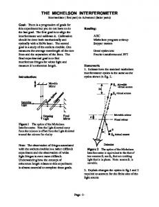
5. NUMERICAL RESULTS The validation of the cube-corner shift evaluation method was performed on the CNES interferometer breadboard (§ 4.1) in several phases. At each alignment step the four needed interferograms were successively recorded in the IHOS focal plane, then processed in quasi-real time in order to estimate the current values of the (y0, z0) and (y’1, z’1) parameters, respectively defining the next translation movements to apply to the fixed cube-corner and laser detection unit, by means of their micrometric tables. The method is illustrated on the Figure 7, which corresponds to the end of the IHOS geometrical prealignment. The upper chart presents the OPD curves computed from the four interferograms acquired at the IASI pixels locations, while the lower charts show the resulting cube-corner trajectory, projected on the horizontal and vertical planes according to the relations (14). The estimated lateral shifts fitted from those trajectories are the following : Constant shifts (shear) Linear shifts (scanning axis alignment)
y0 = -17 µm and z0 = +36 µm. y’1 = +59 µm and z’1 = +22 µm.
Thus a slight re-alignment of the interferometer components looks necessary. The OPD curves on Figure 7 also show residual oscillations which directly are proportional to the CCA speed variations coupled with the electronic delay difference between the main acquisition chain and the RPD electronics, thus providing an useful method to optimize these last parameters.
Figure 7 : OPD and cube-corners lateral shifts at IHOS initial alignment step
Figure 8 corresponds to a more advanced step of the interferometer alignment procedure. It can be seen that the four OPD curves now are almost merged (oscillatory terms are no longer visible, due to a better compensation of the electronic delays), while the lateral shift values averaged on the whole cube-corner trajectory are the following : Constant shifts (shear) Linear shifts
y0 = +1.6 µm and z0 = +8.5 µm. y’1 = -1.4 µm and z’1 = +2 µm.
Thus the constant shifts are compliant with the requirements, and the cube-corner scanning axis is now quasi-parallel to the IHOS optical axis (better than 200 µrad). The convergence of the alignment was confirmed through the four obtained IHOS Line-Shape functions (ILS, see their definition in the Appendix) showing a remarkable symmetry. The global measurement uncertainty is depicted by the error bars displayed on the Figure 8, which are estimated by means of the relations (15). The attained accuracy does not exceed 1.2 µm whatever the cube-corner axial position, and most probably corresponds to a pixel de-correlation caused by one or several of the following error sources : • Positioning accuracy of the IASI pixels in the IHOS focal plane.
• • • • • • •
Mechanical stability* of the breadboard during the four pixel acquisitions (performed successively). Angular diameter of the used detector. Spectral width of the He-Ne laser. Spectral and radiometric stability of the He-Ne laser. Signal-to-Noise ratio of the detection unit. Optical delay originating from the beamsplitter coatings and manufacturing errors. Misalignment of the reference laser beam coupled with cube-corner constant shifts.
Figure 8 : OPD and cube-corners lateral shifts at an IHOS intermediate alignment step
6. CONCLUSION In this paper, we have reviewed the basic principles of an “OPD Measurement Device” (OMD), that may be used to characterize the cube-corners shear and scanning axis parallelism errors of the IASI interferometer. The OMD basically is constituted of a monochromatic light source (e.g. a laser), associated with a detection unit located in the IHOS focal plane. The cube-corner apparent trajectory is retrieved from a specific data processing of four interferograms acquired in the interferometer Field of View, corresponding to the IASI instrument pixels. Then the geometrical misalignments of the cubecorners are accurately estimated using a double Fourier-transform algorithm. The envisaged method was experimented on the IHOS functional breadboard assembled in the CNES laboratories, and the test results presented herein show a good convergence toward the ideal geometrical adjustment of the interferometer. This method is now considered as validated and shall be utilized during the ground alignment of all the future IHOS models.
*
including oscillatory shifts resulting from micro-vibrations generated by the cube-corner driving mechanism or the test set up. Obviously the measurement accuracy will be improved if the four interferograms acquisitions are performed simultaneously.
REFERENCES 1. 2. 3. 4. 5.
P. Javelle, F. Cayla, “IASI instrument overview”, Proceedings of the SPIE, Europto series, vol. 2209, pp. 14-23, 1994 K. Dohlen, F. Hénault, D. Scheidel, D. Siméoni, F. Cayla, G. Chalon, P. Javelle, “Infrared Atmospheric Sounding Interferometer”, Proceedings of the 5th Workshop on ASSFTS, November 30th - December 2nd, 1994, Tokyo F. Hénault, C. Buil, B. Chidaine, D. Scheidel, “Spaceborne infra-red interferometer of the IASI instrument”, Proceedings of the SPIE, vol. 3437, pp. 192-202, 1998 J. Kauppinen, P. Saarinen, “Line-shape distortions in misaligned cube corner interferometers”, Applied optics, Vol. 31, n° 1, January 1992 M. Takeda, H. Ina, S. Koyabashi, “Fourier-transform method of fringe-pattern analysis for computer-based topography and interferometry ”, J. Opt. Soc. Am. A, vol. 72, pp 156-160 (1982)
APPENDIX : OPD RETRIEVAL FROM THE INTERFEROGRAMS The basic principle of the OPD retrieval consists in a specific data processing of the fringe patterns created by the IASI interferometer. Whatever the pixel location in the IHOS Field of View, the interferograms I(ξ) expressed in relation (6) may be rewritten using complex exponential numbers :
I( ξ ) =
2iπσ ξ + δ (u, v) - 2iπσ 0 ξ + δξ (u, v) 1 ξ 0 T(σ 0 ) C(σ 0 ) B 0 (ξ ) e +e 2
(A1)
or (bold characters denoting complex items and * their complex conjugates) :
I( ξ ) =
1 2
V * (ξ , u, v) e 2iπσ 0 ξ + V (ξ , u, v) e - 2iπσ 0 ξ σ0 σ0
(A2)
where Vσ (ξ , u, v) will be the self-apodization function of the interferogram, defined as : 0
Vσ 0 (ξ , u, v) = T(σ 0 ) C(σ 0 ) B0 (ξ ) e
- 2iπσ 0δξ (u, v)
(A3)
Physically Vσ (ξ , u, v) is the envelope of the monochromatic interferogram (see Figure 9), varying with the axial position 0 of the moving cube-corner and FoV incidence angles u and v, while its phase directly is proportional to the searched in-field OPD variations δξ(u,v). This phase may be deduced from the recorded interferogram I(ξ) using a double Fourier-transform algorithm5, which is divided into three main steps as summarized in the Figure 9. 1) The first step consists in computing the inverse Fourier-transform of the recorded interferogram I(ξ). The resulting spectrum S σ (σ , u, v) shows two symmetrical functions respectively centered on the -σ0 and σ0 wavenumbers, which 0 correspond to the time modulation of the recorded interferogram :
{
}
S σ 0 (σ , u, v) = FT -1 [ I(ξ)](σ , u, v) = ILS σ 0 (σ − σ 0 , u, v) + ILS σ 0 (-σ − σ 0 , u, v) / 2
(A4)
where ILS σ (σ , u, v) is the Line-Shape function of the interferometer (ILS), representing its spectral response to an 0 incident monochromatic beam at the wavenumber σ0, as a function of the neighboring wavenumbers σ. The ILS is obtained through the inverse Fourier transform of the self-apodization function Vσ (ξ , u, v) defined in the (A3) relationship : 0
[
ILSσ0 (σ , u, v) = FT-1 Vσ0 (ξ , u, v)
]
(A5)
2) Then, shifting S σ (σ , u, v) of -σ0 and multiplying the result by a boxcar function of width σ0, herein denoted Bσ (σ) , in 0 0 order to cancel the symmetrical ILS, leads to the true spectral response of the interferometer. This operation corresponds to the removal of the time carrier frequency in the interferogram domain :
ILS σ 0 (σ , u, v) = 2 Bσ 0 (σ ) S σ 0 (σ + σ 0 , u, v)
(A6)
3) The direct Fourier-transform of the ILS finally provides the complex self-apodization function Vσ (ξ , u, v) : 0
[
Vσ 0 (ξ , u, v) = FT ILS σ 0 (σ , u, v )
]
(A7)
Finally the in-field OPD variations δξ(u,v) are obtained through a simple inversion of the relation (A3). Here Real[] and Im[] are respectively denoting the extraction of real and imaginary parts :
δξ ( u,v) = −
[
] ]
Im V (ξ ,u,v) σ0 Arctan 2πσ 0 Real Vσ0 (ξ ,u,v) 1
[
(A8)
Hence the OPD variations δξ(u,v) can directly be deduced from the acquired interferograms I(ξ) at each sampling point, provided that the σ0 parameter is known with a sufficient accuracy. SPECTRUM
INTERFEROGRAM
ILS FT
-1
ξ (cm)
0
- σ0
SELF-APODIZATION FUNCTION
0
σ (cm
-1
σ (cm
-1
RECENTRED SPECTRUM ILS
Module (envelope)
FT
Real ξ (cm) Imaginary
)
σ0
0
0
Phase (proportional to the OPD)
Figure 9 : OPD retrieval from the acquired interferograms
)
APPENDIX : LINEAR SHIFT RETRIEVAL FROM ILS CENTROIDS Any misalignment of the IHOS interferometric axis will result in a spectral shift dσi of the actual ILS centroïd. The basic principle of the method is then to correlate the different centroïd shifts which will be measured on four pixels located at the corners of a rectangle centred on the IHOS optical axis (see the Figure 10). As the ILS centroïds directly are determined from the acquired interferograms, the main difference with respect to the principal method essentially consists in data processing. v ILS 2
ILS 1
d σ2
d σ1 σ0
σ0
Pixel 2
Pixel 1 Interferometric axis u Optical axis ILS 4
ILS 3
d σ4
d σ3 σ0
σ0
Pixel 3
Pixel 4
Figure 10 : ILS centroïd shifts in the IHOS field of view For each pixel, the theoretical expression of the centroïd shift dσi is related to the slope of its in-field OPD variations δi(ξ), as illustrated in the Figure 11. We then have :
dσ i = σ 0
∂ δ i (ξ ) ∂ξ
(1 ≤ i ≤ 4)
(B1)
and the four centroïd shifts dσi can be obtained from a second-order development of the relations (11) and (B1), leading to : dσ 1
σ0 dσ 2 σ0 dσ 3 σ0 dσ 4 σ0 where :
≈
dσ 0
−
1
{u
2
+ v 2 } + 2 u y' + 2 v z'
1 P p 1 p σ0 2 P dσ 0 1 2 ≈ − {u P + v 2P } − 2 u p y'1 + 2 v p z'1 2 σ0 dσ 0 1 2 ≈ − {u P + v 2P } - 2 u p y'1 - 2 v p z'1 2 σ0 dσ 0 1 2 ≈ − {u P + v 2P } + 2 u p y'1 - 2 v p z'1 2 σ0
dσ 0
σ0
≈−
{
}
1 2 u0 y1 v0 z1 u0 + v20 - 2 −2 2 ξMax ξMax
(pixel 1) (pixel 2)
(B2)
(pixel 3) (pixel 4)
(B3)
Using the same resolution procedure than in § 3.3.1 finally yields the expression of the interferometric axis coefficients y’1 and z’1, solved in a least-square sense : y'1 = z'1 =
d σ 1 − dσ 2 − d σ 3 + d σ 4
σ0
dσ 1 + dσ 2 − dσ 3 − dσ 4
σ0
× ×
ξ Max 8 up
(B4)
ξ Max 8 vp
Recentred ILS wrt σ 0
Optical Path Difference (OPD) δ ξ (u,v)
Interferogram envelope
FT
OPD slope
ξ (cm)
0
Figure 11 : Phase-corrected ILS centroïd
σ (cm 0
-1
)