David Draper, Antonio Pereira,. Pedro Prado, Andrea Saltelli,. Ryan Cheal, Sonsoles Eguilior,. Bruno Mendes, and Stefano Tarantola. Final Report: Version 3.0, ...
GESAMAC: Conceptual and Computational Tools to Assess the Long-Term Risk from Nuclear Waste Disposal in the Geosphere
David Draper, Antonio Pereira, Pedro Prado, Andrea Saltelli, Ryan Cheal, Sonsoles Eguilior, Bruno Mendes, and Stefano Tarantola
Final Report: Version 3.0, December 1998
Brussels: European Commission EUR 19113 EN (90 pages)
Table of Contents 1
EXECUTIVE SUMMARY
1
2
INTRODUCTION
3
OBJECTIVES WORK PROGRAM
4 5
METHODOLOGY
6
GEOSPHERE MODELLING
6
2.1 2.2 3 3.1
3.1.1 3.1.2 3.1.3 3.2
SENSITIVITY ANALYSIS
3.2.1 3.2.2 3.2.3 3.2.4 3.3
Introduction: the importance of prediction
PARALLEL MONTE CARLO DRIVER
3.4.1 3.4.2 3.4.3 3.4.4 3.4.5
4
The sensitivity indices of Sobol’ Fourier amplitude sensitivity test (FAST) The extended FAST The final SA analysis for GESAMAC
MODEL UNCERTAINTY
3.3.1 3.4
Introduction One-Dimension Transport code Two-Dimension Transport code
Introduction Description of the Program The program environment Performance considerations Correlation between parameters in Monte Carlo calculation
GLOBAL APPROACH IN GESAMAC. THE LEVEL E/G TEST CASE
6 7 14 19 19 21 25 29 30 30 33 33 34 35 35 37
39
Table of Contents (continued) 4.1 4.2 4.3
LEVEL E/G. GENERAL FRAMEWORK OBJECTIVES OF THE LEVEL E/G TEST CASE SCENARIO APPROACH
4.3.1 4.3.2 4.4
SCENARIO PROPERTIES
4.4.1 4.4.2 4.4.3 4.5
Uncertainty calculations Challenges to the Bayesian approach A Model Uncertainty Audit
SENSITIVITY ANALYSIS
4.7.1 4.7.2
4.8
Simulations performed
UNCERTAINTY FRAMEWORK IN GESAMAC
4.6.1 4.6.2 4.6.3 4.7
Scenario Probabilities Physico-chemical reactions versus scenarios Level E/G Data Set
RUNNING THE TEST CASE
4.5.1 4.6
Macro- and Micro- Scenarios Micro-Scenarios: structural assumptions
Initial SA results for maximum dose SA results for total annual dose in the REF scenario
39 39 40 41 44 50 50 51 53 54 55 55 57 57 58 63 63 71
MC DRIVER
75
5
CONCLUSIONS
77
6
REFERENCES
81
LITERATURE CONTRIBUTED BY THE GESAMAC PROJECT OTHER REFERENCES
81 82
6.1 6.2
1
EXECUTIVE SUMMARY
This final technical report details findings from the studies conducted between January 1996 and the end of 1998 in the Project GESAMAC (GEosphere modelling, geosphere Sensitivity Analysis, Model uncertainty in geosphere modelling, Advanced Computing in stochastic geosphere simulation). GESAMAC is a shared cost action (FI4W/CT95/0017) defined in the framework of the IV RTD EC-Program in the field of "Nuclear Fission Safety" in the area of radioactive waste management and disposal and decommissioning. The aim of GESAMAC is to tackle areas of uncertainty, and to develop some conceptual, methodological and computational tools of potential use in actual safety analysis for radioactive waste disposal systems. Four partners covering four different areas of knowledge have joined together to meet the objectives of the project: •
Geosphere Transport Modelling (CIEMAT-DIAE, Spain)
•
Sensitivity Analysis (JRC-ISIS, EC)
•
Model Uncertainty (University of Bath, UK)
•
Parallel MC Driver (University of Stockholm, Dept. Of Physics, Sweden)
Both the long time frames required to assess performance of underground disposal systems for radioactive waste and the variability associated with natural open systems engender different types and sources of uncertainty. GESAMAC offers a conceptual framework that can account for all sources of uncertainty that arise in the simulation of such complex systems as underground disposal. It considers uncertainty in the following simulation components: past data, parameters, structure, scenarios, future observables, and predictions. We have applied our framework to a generic and synthetic nuclear disposal system, placing special emphasis on the geosphere subsystem and focusing on scenario and parametric uncertainties. For stochastic simulation of the system, a parallel Monte Carlo driver has been developed and used to produce stochastic assessment of the performance of the system. The results have been used for uncertainty and sensitivity analysis, in which we applied new quantitative methods that were developed during the project. GESAMAC has provided to the scientific/policy analysis community -
A new method for global sensitivity analysis of model output based on the Fourier Amplitude Sensitivity Test (FAST). Classical sensitivity analysis (SA) estimators based on linear coefficients can cause false interpretation of the results and lead to errors in the decision making process. The new method has been named Extended FAST because of its capacity to evaluate total effect indices for any uncertainty factor in the model under analysis (the classical FAST estimates the main or first order effect only). It also makes it possible to analyse the importance of groups of factors which, properly chosen, can be associated with a particular subsystem, and therefore to assess the relevance of different subsystems over time. The new SA methods have implications that are both epistemic (i.e., pertaining to the scientific method) and political (i.e., linked to policy implementation for the management of risk). One such implication is in the issue of the “relevance” of a model.
-
A conceptual framework to account for all sources of uncertainty in simulation problems of complex systems. The Bayesian approach followed has been applied to a hypothetical nuclear disposal system (which we have called the Level E/G test case). The uncertainty framework combined with the new sensitivity methods provides an innovative method for the analysis of complex models such as those 1
involving disposal systems. These models usually are strongly non-linear and non-additive - especially when scenario uncertainty, an essential constituent of the problem, is incorporated into the analysis. Uncertainties over/in scenarios can now be evaluated and the importance of alternative weights between scenarios to the final results can be shown. -
An additional tool/frame of potential use in communicating safety assessment results to different fora (e.g., politicians or the general public). At present, risk communication and public perception of safety are key issues for the nuclear fuel industry. In some countries, they are the most important issues with which radioactive waste management programs contend.
-
A parallel Monte Carlo driver for stochastic simulations of complex systems which takes advantage of the high performance of parallel computing environments to optimise the efficiency of the simulation. It has been tested with the Level E/G test case and the associated software is available for interested users.
-
A simple research model of a synthetic nuclear disposal system with particular emphasis on the geosphere sub-system. The one-dimensional code GTMCHEM is not far away from the geosphere models used in performance assessment studies published so far. However, it incorporates additional physico/chemical simple reactions to the advective-dispersive transport equation. GTMCHEM also includes two additional modules for the near field and the biosphere subsystems, which define the “system model” for Monte Carlo simulation over scenarios.
-
A test case (Level E/G) for assessing the methodologies and tools developed and/or used in the project.
2
2
INTRODUCTION
During the last decades, various governments and organisations around the world have made important efforts in the area of radioactive waste management. Despite those efforts, a solution for the final part of the nuclear fuel cycle remains today the unresolved issue of the nuclear field. Of the diverse solutions initially proposed, most have opted for the geological disposal of nuclear waste. During the last fifteen years, different countries have performed initial repository safety and/or performance assessment studies of their particular disposal concepts, each of which had different aims, level of detail, etc. Some of those studies have been published and are available in the open literature (SKB-91, TVO-92, SKI Site-94, AECL- 94, TILA-96, etc.). The safety assessment of radioactive waste disposal systems is one area of high priority in the program of the Organisation for Economic Co-operation and Development (OECD) Nuclear Energy Agency (NEA). The NEA's Radioactive Waste Management Committee (RWMC) and its Performance Assessment Advisory Group (PAAG) and Co-ordinating Group on Site Evaluation and Design of Experiments (SEDE) are committed to promoting co-operation among OECD member countries. In 1994, the Working Group on Integrated Performance Assessment of Deep Repositories (IPAG) was set up under the PAAG to provide a forum to discuss Performance Assessment (PA) and to examine the overall status of PA. IPAG’s first goal was to examine and review existing PA studies in order to establish the current state of the art and to shed light on what could or should be done in future studies. Although the studies analysed were heterogeneous with respect to aims, resources, disposal system, or geological media, the review represented the first attempt to extract from a multi-disciplinary field of inquiry observations, conclusions, and recommendations for the future. The 12 observations and recommendations reported in that document (NEA/OECD, 1997) link directly or indirectly to the objectives of GESAMAC. In particular, we have focused on those related to sensitivity and uncertainty analysis (UA), the scenarios approach and the geosphere barrier. Rather than considering the treatment of uncertainty as a separate chapter, the IPAG report incorporated it as an integral element of Performance Assessment, making a distinction between the different kinds of uncertainty and their quantification according to different and complementary approaches. It is conventional for PA studies to use Probabilistic System Assessment (PSA) codes to analyse the performance of nuclear waste disposal, and complementary to the deterministic approaches of the system. PSA codes help to quantify the uncertainty in performance assessment studies and to gauge the sensitivity of the different subsystems and/or variables included. The codes were strongly promoted thirteen years ago by the Probabilistic System Assessment Code (PSAC) User Group, an international working party established in 1985 by the NEA. In particular, computer-based Monte Carlo methodology is usually used to estimate the effects of the disposal over wide combinations of the input parameters. With reference to the geosphere barrier, the above-mentioned report described the role of the geosphere as follows: "The geosphere is a key component in any deep geological disposal system as it both protects and preserves the wastes and engineered barrier system, and may also retard and disperse contaminant releases". It seems reasonable to think, however, that the role of the different barriers involved in a deep geological disposal system may change over time, and that if in the short term the main role could be played by the near field subsystem, over time this role may well move to the geosphere. In this framework, GESAMAC was born. The project aims to simulate, in a stochastic framework where sensitivity and uncertainty analyses of the model outputs are feasible, the transport of nuclides released from a vault through the geosphere up to the biosphere. GESAMAC is the acronym of GEosphere modelling, 3
geosphere Sensitivity Analysis, Model uncertainty in geosphere modelling, Advanced Computing in stochastic geosphere simulation. It is a shared cost action (FI4W/CT95/0017) defined in the framework of the IV RTD EC-Program on Nuclear Fission Safety in the area of Radioactive Waste Management and disposal and decommissioning (GESAMAC, 1995). The project started in January 1996 and finished at the end of 1998.
2.1 OBJECTIVES The goal of GESAMAC is “to tackle areas of uncertainty, and to develop some conceptual, methodological and computational tools which can be of use in actual safety analysis case studies” (GESAMAC, 1995). GESAMAC intends to use the geosphere model to study and perform a fully quantitative synthesis of all sources of uncertainty (scenario, structural, parametric and predictive) and, where they apply, to use variance-decomposition methods in sensitivity analysis. To this end, GESAMAC combines four technical areas of knowledge covered by the four partners involved in the project: §
The first area of knowledge pertains to the system to be modelled and studied; namely, the transport and retardation of the nuclides released from an underground radioactive waste disposal facility, through the geosphere up to the biosphere where the impact is computed as doses to humans. This area connects to the others by use of Monte Carlo simulation of this system over a set of scenarios to produce a set of outputs to be used for sensitivity and uncertainty analysis.
§
The second area is the sensitivity analysis of the model outputs. Innovative quantitative methods for global sensitivity analysis based on “variance decomposition techniques” have been applied. This improves upon classical qualitative measures based on regression/correlation methods, which can cause false interpretation of the results and lead to errors in the decision making process. Such problems often occur with complex models, particularly if they are strongly non-linear and non-additive, as with the radioactive waste disposal systems considered here.
§
The third area of knowledge is model uncertainty. The aim is to combine and propagate the different sources of uncertainty (scenario, structural, parametric and predictive) instead of following the more traditional approach based on studying the likeliest scenario.
§
The fourth area aims to combine the advances of high performance computers with the parallel nature of Monte Carlo simulation. We have developed a parallel Monte Carlo driver to optimise the efficiency of the simulation of complex systems.
The four technical areas outlined were covered by the CIEMAT-DIAE (Spain), the JRC-ISIS EC (Italy), the University of Bath (UK), and the University of Stockholm (Sweden), respectively. In order to demonstrate the applicability of the methodology proposed we developed a test case during the project that allowed us to combine those technical areas of research in a global trial of the project. In the following chapters of this report, we describe each of these areas in detail.
4
GEsophere Modelling
Sensitivity Analysis
Model Uncertainty
Parallel MC Driver
Figure 2.1.1. General framework of GESAMAC
2.2 WORK PROGRAM It was mentioned above that GESAMAC was a three years project with four organisations involved, where each of the partners has specific areas of concern within the project. As co-ordinator, CIEMAT has been in charge of the administrative/financial and scientific/technical aspects of the contract. CIEMAT also organised the regular project meetings. The work program established (GESAMAC, 1995) addressed the development of methods and tools with potential application to the current performance assessment studies of geological disposal of radioactive wastes. To achieve this, however, the methods proposed and the associated tools being developed required a system in which they could be tested. At the end of the first project year, it was deemed useful to define a test case for that purpose. This was the origin of the Level E/G test case, which initially was not scheduled as one of the project activities. The success of this approach was so great that it became a focal point for the entire project. The aim of the work programme was to devise a methodology for the analysis of complex systems. Here the system model considered was a radioactive waste disposal system. We performed Monte Carlo simulation to produce a set of model outputs upon which innovative sensitivity analysis and model uncertainty techniques could be applied. The model outputs of interest are the doses through time that arise by the groundwater transport of the radionuclides through the geosphere up to the biosphere, once the near field barriers have lost their containment capacity.
5
3
METHODOLOGY
The methodology proposed by GESAMAC basically consists in the MC simulation of a system model (in this case a radioactive waste disposal system) in which global SA and UA are applied over the model outputs. The following sections summarise (1) each separate aspect of the work performed and (2) how they have been integrated through a hypothetical test case.
3.1 GEOSPHERE MODELLING This area of work concerns models of radionuclide migration by taking into account the solid-liquid interaction phenomena through the migration process. It has investigated the groundwater transport of nuclides through a multilayer system in one and two dimensions, and has studied the effects of parameters and model assumptions on the predictions of the model. The model concentrates on those model assumptions that relate to the physico-chemical reactions between the liquid and solid phases. In order to weight the impact of different conceptual assumptions, a model has been implemented to describe the liquid phase-solid phase interaction. The uncertainties in model parameters and model assumptions have been investigated by a combination of Monte Carlo methodologies and Bayesian logic, which allows for uncertainty and sensitivity analysis.
3.1.1 Introduction The geological disposal of radioactive waste is based on the multi-barrier system concept: both man made and natural barriers. The importance of each barrier involved depends on several factors; for example, the kind of waste considered, the disposal concept, the scenario taken into account, and the time span under consideration. In the case of the geosphere barrier, its role depends on the safety assessment study being considered1. The geosphere is the most important among the various barriers, which isolate the waste from the biosphere. In the short term it maintains its particular physico-chemical environmental conditions around the underground facility to permit the correct operation of engineering barriers. In the long-term - once the nuclides are released from the vault - it acts as a physical and chemical barrier to the pollutants. According to this framework, the transport of nuclides by the groundwater is one of the most probable transfer pathways of nuclides from the vault to the biosphere, and is therefore one important component in performance assessment studies of the geological disposal systems. The performance assessment of the waste disposal system requires the formulation of mathematical simulation models, based on conceptualisations of the different subsystems involved, in particular the hydrogeological system. This kind of analysis has to consider the many uncertainties that arise mainly from an incomplete knowledge of the system and from the system variability. The Probabilistic System Assessment (PSA) Codes developed by different countries over the past years intend to quantify those uncertainties. One way of realising a PSA is by using a Monte Carlo methodology and running the assessment model over a wide combination of input parameters. Therefore, the barrier sub-models used by the PSA codes must be robust and computationally efficient. For this purpose a one-dimensional description of the transport phenomena is generally adopted.
1
SKB 91. Final disposal of spent nuclear fuel. Importance of the bedrock for safety: “The primary function of the rock is to provide stable mechanical and chemical conditions over a long period of time so that long-term performance of the engineered barriers is not jeopardised”
6
GESAMAC built on the previous work (Prado 1992, Prado et al. 1991, Saltelli et al. 1989) to produce a new release of the code, concentrating on the geochemical part of the radionuclide groundwater transport problem. GESAMAC intends to use the geosphere model (first in one dimension and then in two dimensions) to study and perform a fully quantitative synthesis of all sources of uncertainty (scenario, structural, parametric and predictive) and, when possible, to try a quantitative variance-decomposition approach in sensitivity analysis.
3.1.2 One-Dimension Transport code 3.1.2.1 GTM-1 Computer Code GTM-1, written in FORTRAN-77, describes a column of porous material (1D), whose properties can change along the pathway. Within the column, groundwater transports the nuclides released from a source term. The transport equation is approximated by the finite differences technique following the implicit Crank-Nicolson numerical scheme. The advective/dispersive transport equation solved by the code has the following form ∂C ∂ C ∂C =D −V − R n λn C n + R n −1 λn− 1 C n− 1 2 ∂t ∂X ∂X n
Rn
2
n
n
(3.1.1)
where, C is the concentration of solute in solution [mols/m3]; R is a retention factor of the nuclides in solution by the solid phase [-]; D is the hydrodynamic dispersion coefficient [m2/y]; V is the groundwater pore velocity [m/y]; t and X are time [y] and space [m] respectively and λ represents the radioactive decay constant [1/y]. The upper indices refer to the nuclide considered in the radioactive decay chain ('n' for the daughter and 'n-1' for the parent) The performance assessment study of complex systems is customarily carried out by breaking down the total system into separate compartments. In the case of the radioactive waste disposal systems, a common breakdown consist in a ‘near field’, a ‘far field’ and a ‘biosphere’ sub-systems. Initially developed for inclusion into a PSA Monte Carlo code, GTM1 includes the three main models usually considered in the analysis of underground repository systems: a simple source term module, the geosphere (GTM properly), and a simple biosphere module. The code was verified by comparison of the numerical results with analytical solutions (Robinson and Hodgkinson 1987) and against the international PSACOIN benchmark exercises (NEA PSAC User Group 1989 and 1990). More detailed information about this version of the code can be found in the ‘User’s manual for the GTM-1 computer code’ (Prado 1992), and other papers (see, e.g., Prado et al, 1991) included in the References section of the current document. 3.1.2.2 GTMCHEM Computer Code In transport phenomena involving interaction between the migrating species and a stationary phase, it is often assumed that the reaction by which the immobilised reactants are formed proceeds very rapidly compared to the transport process. When the flow is sufficiently slow, it may be permissible to assume that equilibrium is maintained at all times and so the equilibrium relationship, which links the various reactants, can be directly substituted into the transport equation. However in many cases the equilibrium concept is no longer valid and the process of adsorption can be described properly only through considering kinetic reactions, which are coupled to the main transport equation of the migrating species.
7
The linear and reversible equilibrium adsorption isotherm (‘K d’ concept) was the only phenomena considered in GTM1. The new version, named GTMCHEM, retains most of the original structure and capabilities of GTM1 and incorporates other kinds of reactions between the solid and liquid phases. The physico-chemical reactions considered are included into the transport equation separately from the advective/dispersive part of the equation, as a source/sink term. GTMCHEM retains from GTM1 the three general sub-models usually considered for underground radioactive waste disposal systems, as separate subroutines in order to ease for the user the inclusion of new sub-models. It is assumed that the column of porous material is completely saturated with water. The advection-dispersion-adsorption model is used to simulate solute transport with chemical reactions in a porous media. The general 1D mass balance equation for radionuclide movement has the form n ∂ ( ciθ i ) ∂ ∂ ∂ = − [vi ciθ i ] + Di ( ciθ i ) + Siext + ∑ Sijint ∂t ∂x ∂x ∂x j =1
IC : ci ( x , t = 0) = 0 BC : c i ( x = 0, t ) = c i0
(3.1.2)
Here ci is the concentration [ML-3] of the participant i; v i and Di represent the average groundwater velocity [LT-1] and the hydrodynamic dispersion coefficient [L2T-1] respectively; θi is the volume fraction containing the participant i [-]; and Siext and Sijint depict the external and internal source/sink terms respectively with i and j as the indices of the participants. The external source/sink term (Siext) contains all changes in concentration of participants i due to processes which are independent of the concentration of other participants (i.e., radioactive decay or biodegradation). The internal sink/source term (Sijint) includes all concentration changes that involve other participants (i.e., chemical reactions or increase due to parents decay). The 'n' partial differential equations are coupled by internal sources/sinks (Sijint = - Sjiint) describing the exchange rates of participants from phase j to phase i (heterogeneous reaction) or the transformation rates of participant j to participant i within a single phase (homogeneous reaction). Therefore, there will be as many equations to solve as elements considered in the problem, i.e., not only the nuclides released from the repository, but also the elements transported in solution by the groundwater and/or in the solid phase. The final problem to be solved consists of a system of partial differential equations coupled by the radioactive decay and/or by the chemical reactions considered between the elements involved. Those phenomena are described below. Radioactive decay: ext
= −λi C i
int ij
= λjC j
Si S
(3.1.3)
Here i and j indicate the participant in the mass balance equation and its parent nuclide respectively, λi,j are the radioactive decay constants [yr -1] and Ci , Cj are heir concentration values [mols]. Heterogeneous adsorption with a linear isotherm in equilibrium: If we denote by A the participant in solution and by A' the quantity of the participant adsorbed in the solid phase, the associated mass balance equations can be written as follows 8
∂C A ∂C ∂ 2 C A S AA' = −v A + D − ∂t ∂x ∂x 2 θ1 ∂C A' S AA' = ∂t θ2
(3.1.4)
where θ1 and θ2 are the volume fraction of liquid and solid phases respectively and SAA’ is the adsorption source/sink term (SAA’ = -SA’A). If equilibrium is assumed between CA and CA’ and the adsorption process is represented by a simple linear isotherm model, we can write ∂C A' dC A' ∂CA = ∂t dC A ∂t
(3.1.5)
dC A' = Kd dC A
(3.1.6)
with
where 'Kd' is the distribution coefficient [m3/kg]. From Equation 3.1.4 we can write S AA' = θ 2
∂C A ' ∂t
(3.1.7)
and therefore, S AA' = θ 2 K d
∂C A ∂t
(3.1.8)
so that by substitution in equation 3.1.4 we obtain RA
∂C A ∂C ∂ 2 CA = −v ⋅ A + D ⋅ ∂t ∂x ∂x 2
(3.1.9)
where RA represents the retention factor for the element A, RA = 1 +
θ2 Kd θ1
(3.1.10)
Homogeneous equilibrium: In this case, if equilibrium is assumed between the participants i and j they must satisfy the relationship Ci = KequilC j
(3.1.11)
where Kequil represents the equilibrium constant. In this case, an algebraic equation that relates the elements in equilibrium is added to the differential transport equation. Therefore the initial system of two coupled
9
differential equations and an algebraic equation can be reduced to a differential equation plus an algebraic equation, simplifying the resolution of the system. Let us consider equilibrium in solution between the participants A and B and also the adsorption reactions for both of them (A' and B' respectively) and radioactive decay. The equation system to be solved can be written as follows: Mass balance system ∂C A ∂C A ∂ 2 C A S1 S3 = −v +D − − − λA C A ∂t ∂x ∂x 2 θ1 θ1 ∂C B ∂C B ∂ 2 C B S 2 S3 = −v +D − + − λA C B 2 ∂t ∂x ∂x θ1 θ 1 ∂ C A ' S1 = − λ ACA' ∂t θ2
(3.1.12)
∂ C B ' S2 = − λ ACB' ∂t θ2
Slow adsorption ∂ ∂ CA ' = K A C A ∂t ∂t ∂ ∂ CB ' = K B CB ∂t ∂t
(3.1.13)
CB = K ABC A
(3.1.14)
Chemical equilibrium
Initial and boundary conditions:
C A ( x, t = 0) = C B ( x, t = 0) = C A' ( x , t = 0) = C B' ( x , t = 0) = 0 C A ( x = 0, t ) = C A0 C B ( x = 0, t ) = C B0 C A' ( x = 0, t ) = 0 C B' ( x = 0, t ) = 0
0 0 C B = K ABC A
(3.1.15)
where S1 and S2 are the Source/Sink terms for the adsorption reactions and S3 is the Source/Sink term for the equilibrium reaction. From the adsorption equations we can obtain S1 and S2
10
∂C A + θ 2λ AC A' ∂t ∂C S 2 = θ 2 K B B + θ 2λ ACB' ∂t S1 = θ 2 K A
(3.1.16)
and using the relations between CA - CA’ and CB – CB’ ∂C A + θ 2 K Aλ AC A ∂t ∂C B S2 = θ 2 K B + θ 2 K B λAC B ∂t S1 = θ 2 K A
(3.1.17)
The value of S3 cannot be obtained in the same way as S1 and S2. An option is to add the mass balance equations for A and B, obtaining
∂ 2 C A ∂ 2C B ∂C A ∂C B ∂C ∂C + = −v A + B + D + − 2 ∂t ∂t ∂x ∂x 2 ∂x ∂x θ2K A θ1 θ K − 2 B θ1 −
∂C A θ 2 K A λ A C A − − λ AC A − ∂t θ1 ∂C B θ 2 K B λ A C B − − λ AC B ∂t θ1
(3.1.18)
With : IC : CA ( x, t = 0) + CB ( x, t = 0) = 0 BC : C A ( x = 0, t ) + C B ( x = 0, t ) = C 0A + C B0 where the expressions above for S1 and S2 have been substituted. Now if we consider the following equalities CB = K ABC A θ RA = 1 + 2 K A θ1 θ RB = 1 + 2 K B θ1
(3.1.19)
and we perform the appropriate substitutions in the previous equation, we will get the following expression for the mass balance:
(1 + K AB ) ⋅ v ∂CA (1 + K AB ) ⋅ D ∂ 2C A ∂C A =− + − λA C A ∂t [RA + K AB RB ] ∂x [R A + K AB RB ] ∂x 2 With : IC : CA ( x , t = 0) = 0 C 0A + CB0 BC : C A ( x = 0, t ) = 1 + K AB 11
(3.1.20)
In the same way we could obtain the expression for the mass balance in the case of a decay chain (A* → A → ...). In that case the final expression would be: ∂C A ( 1 + K AB ) ⋅ v ∂C A (1 + K AB ) ⋅ D ∂ 2C A =− + − ∂t [RA + K AB RB ] ∂x [RA + K AB RB ] ∂x 2 − λ AC A +
[RA* + K A*B* RB* ] λ C [RA + K AB RB ] A* A*
(3.1.21)
With : IC : CA ( x, t = 0) = 0 BC : C A ( x = 0, t ) =
C 0A + CB0 1 + K AB
Therefore, if chemical equilibrium is considered in the general transport equation, the changes required refer to the retardation factor for another more general expression, 1 1 → RA RA + K AB RB
(3.1.22)
V → (1 + K AB )V D → (1 + K AB ) D
(3.1.23)
where V and D are given by
and the initial and boundary conditions by: IC : CA ( x, t = 0) = 0 BC : C A ( x = 0, t ) =
C 0A + CB0 1 + K AB
(3.1.24)
Then, the final system of equations required to obtain the new concentrations for A and B will be the differential equations written above plus the relationship from equilibrium, which allows us to know the concentration of the element B once we know the concentration of A. Slow chemical reactions (no equilibrium): These kind of chemical reactions (i.e., slow adsorption) are described as kinetic and the Source/Sink term has the following form:
Sijint = − Kij Ci + K jiC j
(3.1.25)
where Kij represents the kinetic rate constants. Each element has as many factors like this as reactions in which it is involved.
12
Combining all the reactions above mentioned, the source/sink term for the transport equation is established. If the reactions considered are •
Homogeneous equilibrium between the participants A and B (CB = KAB·CA)
•
Radioactive decay: A* represents the parent nuclide of A into the decay chain
•
Adsorption: A and B adsorbed into the solid phase by heterogeneous adsorption with a linear equilibrium isotherm (RA and RB)
•
Initial and boundary conditions for A and B:
I .C. :
Ci ( x, t = 0) = 0
i = A, B
B.C. :
C A ( x = 0, t ) = C A0
(3.1.26)
CB ( x = 0, t ) = CB0 the final master equation will be of the form ∂C A ( 1 + K AB ) ⋅ v ∂C A (1 + K AB ) ⋅ DA ∂ 2C A =− + − ∂t [RA + K AB RB ] ∂x [RA + K AB RB ] ∂x 2 − λ AC A +
[R A* + K A*B* RB* ] λ C [RA + K AB RB ] A* A* (3.1.27)
−
n 1 n K C − K JAC J ∑ AJ A ∑ [R A + K AB R B ] J =1 J =1
C B ( x, t ) = K ABC A ( x, t )
with IC : CA ( x, t = 0) = 0 BC : C A ( x = 0, t ) =
C 0A + CB0 1 + K AB
(3.1.28)
where, CA,CB Concentration of the elements A and B in solution [mols]; KAB Equilibrium constant for the homogeneous equilibrium reaction between A and B; Ri Retardation factor for the heterogeneous adsorption reaction with linear equilibrium isotherm; V Groundwater velocity [m/y]; DA Hydrodynamic dispersion coefficient [m2/y]; λi Radioactive decay constant of element i [1/y]; KAi;iA Kinetic rate constants [1/y]; x Space co-ordinate [m]; t Time [y].
13
3.1.2.3 Numerical Approach The final system to be solved consists of a set of partial differential equations coupled through the radioactive decay terms (an element is related to its predecessor) and through the slow chemical reactions (slow reactions in comparison with the advective/dispersive term of the transport equation). To solve the system, a two step procedure without iteration has been followed. This procedure consists of solving first the advective/dispersive part together with the decay and the homogeneous reactions, obtaining an intermediate concentrations quantity (C’). Those values are obtained following the same scheme used in GTM1 (a Finite Differences and Crank-Nicolson scheme). Then those values are used to compute a correction term (∆C) for the concentrations as results of the chemical reactions taken into account. The system of equation can be written as follows: n
(
)
∆C1 = ∑ − k1 j ⋅ C1' + k j1 ⋅ C 'j ⋅ ∆t j =1
(3.1.29)
... n
(
)
∆Cn = ∑ − k nj ⋅ Cn' + k jn ⋅ C 'j ⋅ ∆t j =1
Once the increases in the concentrations from the chemical reactions have been obtained, the new concentration values, after a time step, are updated as follows: Ci = Ci' + ∆Ci
(3.1.30)
The two step approach is correct taking into account the following constraints: a) For slow chemical reactions the error of decoupling the advective/dispersive transport and chemical reactions part is negligible if ∆x ⋅ R < TR v ∆x 2 ⋅ R TD = < TR D TC =
(3.1.31)
where, TR , TC and TD are the time scales for the chemical reactions, the convective and the dispersive transport respectively. b) For heterogeneous reactions, the two-step procedure without iteration results in greater truncation errors than in the homogeneous case but we have a good approximation if the previous conditions are fulfilled. By definition this condition cannot be met for fast exchange (Herzer and Kinzelbach 1989).
3.1.3 Two-Dimension Transport code This task initially scheduled to start at the beginning of the 2nd year project was postponed to the second semester of 1997 in order to use this period to establish the specifications of the Level E/G test case, which was not included in the delineation of the project. The 2D version developed approaches the groundwater transport equation following the random walk method instead of the finite difference approach used in the 1D version. 14
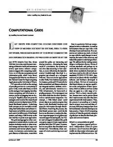
3.1.3.1 Random Walk Approach The movement of particles through the porous medium has a random aspect. Sometimes they move fast through the voids between grains and sometimes they move slowly around grains. The basic idea of the Random Walk (RW) method (Ne-Zheng 1995, Kinzelbach 1986, Prickett et al. 1981) is that the mass transport through porous media may be looked upon as an average result of the movement of a large number of tracer particles. Each particle is engaged in two kinds of coupled movements: 1. Advection: represented by the movement of particles by the groundwater velocity in the flow field. 2. Dispersion: which may be seen as a random fluctuation around the average movement. The result of these two movements is that each particle describes its own random pathway. By considering many individual particles’ paths, a cloud of particles is obtained. This cloud of particles changes from one time to the next as a function of the geological media properties, so the movement of the plume through time can be obtained. Since what we are moving are particles, they can be transformed in concentrations, counting the number of particles per grid cell. Adding or destroying particles can simulate sources and sinks. In two dimensions, the two steps for transport of the particles are first by advection in the direction of the flow field and then by dispersion (X and Y components). The general idea of the RW method is presented in Figure 3.1.1. The advective displacement of a generic particle can be expressed as:
∆ X = V X ∆t
(3.1.32)
∆ Y = VY ∆t V = V X2 + VY2 And the dispersive components are
RX = RL Cosθ − RT Senθ RY = RL Senθ + RT Cosθ tg θ =
(3.1.33)
VY VX
where RRL = RRT =
2α LV∆t V∆t 2α TV∆t V∆t
RNORM (0)
;
RL = RR L * V∆t
(3.1.34) RNORM (0)
15
;
RT = RRT *V∆t
RT* Cosθ
Y
RY R L * Senθ
∆y
( RT Q =S ∆t * V θ ∆x=V x* ∆t
)
∆y=V y* ∆t
2
2 + ∆x
R T* Senθ R L * Cosθ RX X
Figure 3.1.1. Advective (arbitrary flow field direction) and dispersive steps in a Cartesian co-ordinate system Operating with the above equations, the final position of the particle after a time step is obtained by the following equation:
X p, k +1 = X p, k +
∆X
+
RRL ∆ X
−
RRT ∆Y
= Yp ,k +
∆Y
+
RRL ∆Y
+
RRT ∆ X
Y p, k +1
(3.1.35)
where RRL = RRT =
2α LV∆t V∆t 2α TV∆t V∆t
RNORM (0)
;
RL = RR L * V∆t
(3.1.36) RNORM (0)
;
RT = RRT *V∆t
Therefore, the combination of the advective and dispersive movements of the particles results in a random distribution of the pathways generated (see Figure 3.1.2). If space is divided in cells, e.g. into rectangles, the particles falling in each of the cells can be transformed in concentrations: Ci, j (t ) =
∆M * ni, j (t ) N * ne * mi , j * ∆X * ∆Y
Here X, Y
Cartesian co-ordinates (m)
P, k
generic particle p (-) and generic time point k (y)
Vx,Vy
groundwater velocity components (m/y)
α L, α T longitudinal and transverse dispersivities respectively (m) 16
(3.1.37)
∆X, ∆Y displacements caused by advection in X and Y directions respectively (m) Ci,j(t)
concentration in cell i,j at time t (mg/m3)
∆M
total pollutant mass injected (mg)
ni,j
number of particles falling into grid cell (i,j)(-)
ne
effective porosity (-)
mi,j
thickness of grid cell (i,j) (m)
N
number of particles over which ∆M is distributed (-)
Particle trajectories 20,00 15,00 10,00 1
Y (m)
5,00
2 3
0,00
4 5
-5,00 -10,00 -15,00 -20,00 -30
-10
10
30
50
70
90
X (m)
Figure 3.1.2. An example of the pathways described by the advective and dispersive motion of five particles.
An illustration of the concentration plumes obtained after this transformation is shown in the following picture for two different RW simulations: permanent and momentary injections respectively.
17
Plume Evolution (momentary injection) 20 d
40 d
60 d
80 d
Plume Evolution (permanent injection) 20 d
40 d
60 d
80 d
18
3.2 SENSITIVITY ANALYSIS The objective of this part of the GESAMAC project was to develop better sensitivity analysis methods for use in the probabilistic assessment. The work has been successful, as in the end new methods were actually implemented and tested, and several articles published in the literature. We shall describe in the following the path taken in our research work, starting with a brief description of the original methods addressed in the investigation: the Sobol’ method and the FAST sensitivity indices.
3.2.1 The sensitivity indices of Sobol' The sensitivity indices of Sobol' were developed in 1990, based on Sobol's earlier work on the Fourier Haar series (1969). The indices were developed for the purpose of sensitivity analysis, i.e., to estimate the sensitivity of f(X) with respect to different variables or their groups. Let the function f( X) = f( x1 , x 1 ,... , x n ) be defined in the n-dimensional unit cube:
K n = ( x | 0 » = xi » = 1; i = 1,..., n
)
(3.2.1)
It is possible to decompose f(x) into summands of increasing dimensions, as n
f ( x 1 ,..., x n) = f 0 + ∑ f i (x i) + ∑ i =1
∑ 1»= i»= j» = n
(
...+ f 12...n x i , x j , ... x n
(
)
f ij x i , x j +
)
(3.2.2)
provided that f 0 is a constant and the integral of every summand over any of its own variables is zero. A consequence of the above definition is that the variance of the model also can be decomposed into terms of increasing dimensionality: n
D = ∑ Di + ∑ i=1
∑
D ij + ...+ D12...n
(3.2.3)
1»=i»= j»= n
At this point the sensitivity estimates S i1...i s can be introduced: S i1...i s =
D i1... is D
(3.2.4)
It follows that ∑" S i1...i s = 1
(3.2.5)
where the sum with inverted commas notation indicates a sum over all the combinations of indices. The terms Si1,...is are very useful for sensitivity analysis, as they give the fraction of the total variance of f(x) that is attributable to any individual parameter or combination of parameters. In this way, for example, S1 is the main effect of parameter x 1, S12 is the interaction effect, i.e. that part of the output variation due to parameters x 1 and x 2 which cannot be explained by the sum of the effect of parameters x 1 and x 2. Finally 19
the last term S12...n is that fraction of the output variance which cannot be explained by summing terms of lower order. This kind of decomposition is not unique in the treatment of numerical experiments: a variance decomposition identical to Equation (3.2.3) is suggested by Cukier et al. (1978) using the FAST method for sensitivity analysis. FAST (Fourier Amplitude Sensitivity Test) is based on a Fourier transformation (see below). A shortcoming of this method is that when using FAST, calculation usually stops at the main effect terms (see also Liepman and Stephanopoulos 1985). Other investigators have developed sensitivity measures (known as importance measures or correlation ratios) which are also based on fractional contributions of individual model parameters to the output variance. All these measures are amenable to Sobol's sensitivity indices of the first order. In an SA exercise, they would produce the same parameter ranking as would be obtained using the Si's , without interaction and higher order terms. The applicability of these sensitivity estimates is related to the possibility of evaluating the partial variances by multidimensional integrals using Monte Carlo methods. One separate Monte Carlo integral is needed for each term in the series development (Equation 3.2.3), and the number of terms is equal to 2n-1, far too many to be computed even for moderate model dimension n. In factorial design one can usually discount the importance of the higher order interactions, mostly based on assumptions of smoothness and similarity in the response function, up to the point that it is not unusual to estimate the standard error of the main effects or interactions by averaging the (supposedly pure noise) higher order terms (see, e.g., Box, Hunter and Hunter 1978). In numerical experiments, on the other hand, where the models are usually non-linear and the variation in the response is much wider (orders of magnitude), it may happen that the higher order terms are the most important (see an example in Saltelli and Sobol', 1995). Hence their estimation is crucial. One useful property of the sensitivity indices is that variables can be combined together, treating subsets of variables as new variables; thus, for instance, x can be partitioned into v and w, where v contains the variables x1 to xk, and w the remaining (n-k) variables, and the variance of f(x) can then be written as: D = Dv + D w + D v,w
(3.2.6)
This offers an easy solution to the problem of how to evaluate the effect of the large number of higher order terms. For each variable x 1 the total effect term can be computed (Homma and Saltelli 1996, Saltelli et al. 1994): S Ti ≡ S i + S i,u = 1 S u
(3.2.7)
where, Si
is the main effect of x i
Su
is the main effect of x u
Si,u
is the interaction term x1 , x u
xu
is the variable obtained by reducing x of the variable x i
In this way one can estimate the total contribution of each variable to the output variation, and the number of Monte Carlo integrals to be performed is only equal to the number of variables plus one.
20
One general conclusion of this section is that the Sobol' formulation of sensitivity indices is very general and may include as a particular case most of what has been done in SA using decompositions like Equation (3.2.3), as well as several sensitivity measures based on the variables’ fractional contribution to the output variance. In Archer et al. (1997) the Sobol' method, which is based on decomposing the variance of a model output into terms of increasing dimensionality (first order, interaction, higher order) was compared with the classical ANOVA used in experimental design. The genesis of the ANOVA-like decomposition in (physical or biological) experimental design was reviewed briefly, in order to highlight similarities with the methods used for numerical experiments, such as the Sobol' indices and the Fourier Amplitude Sensitivity Test (FAST). The article concluded that the ANOVA decomposition and the decomposition underlying both FAST and Sobol' indices have an identical theoretical foundation. In the same article it was also shown that the bootstrap approach can be used to calculate the error in the numerical estimate of Sobol' indices. The bootstrap is based on the concept of resampling without replacement individual model evaluations used in the Monte Carlo scheme to compute the sensitivity indices. This allows many bootstrap replicas of a given index value to be built, so that a bootstrap distribution can be estimated. In the end, among other statistics, confidence bounds can be attached to the indices themselves (Efron and Stein 1981). All computations of sensitivity indices were made using quasirandom numbers (Sobol' 1967, 1976).
3.2.2 Fourier amplitude sensitivity test (FAST) The FAST method allows the computation of that fraction of the variance of a given model output or function which is due to each input variable. The key idea underlying the method is to apply the ergodic theorem as demonstrated by Weyl (1938). This hypothesis allows the computation of an integral in an ndimensional space through a mono-dimensional integral. Let the function f( X) be defined in the n-dimensional unit cube (Equation 3.2.1). Consider the set of transformations: x i = g i ( sin ( wi _ s)) i = 1,..., n
(3.2.8)
If a linearly independent set of frequencies {w1,...,wk} is chosen (no wi may be obtained as a linear combination of the other frequencies with integer coefficients), when s varies from -∞ to ∞, the vector (x1(s),...,xn(s)) traces out a curve that fills the whole n-dimensional unit cube Kn, so that, following Weyl (1938), the integral f0 =
∫ f( x ) dx1 ... dx n ,
Kn
(3.2.9)
and the integral ˆf = lim T →∞ 1 ∫ T f( x(s))ds . 0 2T - T
are equal.
21
(3.2.10)
Since the numerical computation of integrals like that in Equation (3.2.10) is impossible for an incommensurate set of frequencies, an appropriate set of integer frequencies is used. The consequences of this change is that the curve is no longer a space filling one, but becomes a periodic curve with period 2, and approximate numerical integrations can be made. If these ideas are extended to the computation of variances, the variance of f may be computed through D =
1 π 2 ∫ f ( x(s))ds 2π -π
2 - ˆf 0 ,
(3.2.11)
where this time ˆf = 0
1 π ∫ f( x(s))ds . 2π -π
(3.2.12)
The application of Parseval's theorem to the computation of Equation (3.2.11) allows one to reach the expression: ∞
D = 2 ∑ ( A j2+ B j2 ) ,
(3.2.13)
j=1
where the Aj and the Bj are the common Fourier coefficients of the cosine and the sine series respectively. Following Cukier et al. (1978), the part of this variance due to each individual input variable is the part of the sum in the Equation (3.2.13) extended only to the frequency assigned to each input variable and its harmonics, so that ∞
2
2
2 ∑ ( A p_ wi + B p_ wi ) Si =
p=1
∞
, 2
(3.2.14)
2
2 ∑ ( A j +B j ) j=1
is the fraction of the variance of f due to the input variable x i. The summation in p is meant to include all the harmonics related to the frequency associated with the input variable considered. This coefficient is equal to what is called a "main effect" in factorial design. Unfortunately, the fraction of the total variance due to interactions, i.e., the combined effect due to two variables that cannot be resolved by the sum of individual effects, may not be computed with this technique at present, although Cukier et al. (1978) make some reference to the possibility of computing the contribution of higher order terms (see the next section). The computation of formula (3.2.14) for each input variable needs the evaluation of the function f at a number of points in Kn to compute each Ai and each Bi, i=1,...,n. The first step in the computation of the indices is the selection of the set of integer frequencies. Cukier et al. (1975) provide an algorithm to produce those optimal sets. Those sets are optimal in the sense of being free of interferences until fourth order, and demanding a minimum sample size. This minimum is determined by the Nyquist criterion and is 2⋅wmax+1, where wmax is the maximum frequency in the set. Schaibly and Shuler show (1973) that the results are independent of the assignation of frequencies to the input parameters. The selected points are equally spaced points in the one-dimensional s-space. A study of the errors due the use of integer frequencies is in Cukier et al. (1975).
22
In Saltelli and Bolado (1996) a comparison of the predictions and of the performances of the FAST and Sobol' indices has been realised by mean of a computational experiment. Both indices have been applied to different test cases at different sample sizes and/or at different problem dimensionality. In order to compare the results against exact analytical values the following function is used: n
f = ∏ gi ( xi )
(3.2.15)
i=1
where g i ( xi ) =
| 4 x i 2 | + ai , ai ≥ 0 1 + ai
(3.2.16)
The function f is defined in the n-dimensional unit cube (Equation 3.2.1) and the a's are parameters. Figure 3.2.1 gives plots of the g term for different values of a. The same function, with all a's = 0, was used in Davis and Rabinowitz (1984) to test multidimensional integration. The function (3.2.15 and 3.2.16) has also been used in Saltelli and Sobol (1995a,1995b). 1
For all g functions ∫ g i ( x i ) dx i = 1 0
1
1
0
0
and therefore ∫ ... ∫ f dx 1 ...dx n = 1 The function g i ( xi ) varies as 1
1 1 ≤ g i (x )i ≤ 1 + 1 + ai 1 + ai
(3.2.17)
For this reason the values of the a's determine the relative importance of the input variables (the x's). These plots (and the other contained in the original reference, including an application to the LEVEL E test case, OECD 1989) show that although the computations of the two indices follow quite different routes, they estimate the same statistical entity. This is the main effect contribution to the output variance decomposition in the ANOVA terminology. The two indices tend to yield the same number when estimating main effects. FAST appeared to be computationally more efficient, and is clearly a cheaper method to predict sensitivities associated with main effects. It also seems that FAST is more prone to systematic deviations from the analytical values (bias), perhaps because of the interference problem. Sobol' indices are computationally more expensive, although they converge to the analytical values. Furthermore these indices provide a unique way to estimate the global effect of variables as well as interaction terms of any order.
23
Figure 3.2.1. Comparison of FAST and Sobol' indices for the analytical test function.
The main conclusions of the work described so far are: §
The theoretical foundation of the ANOVA-like decomposition of variance in experimental design and that of the FAST and Sobol' indices is the same.
§
The bootstrap can be used to quantify the error in the numerical estimate of the sensitivity indices.
§
FAST and Sobol' indices of the first order yield the same number, i.e., they are identical in their predictions.
§
FAST is more computationally efficient than Sobol' indices.
§
FAST seems to be biased compared to the Sobol' indices and to the expected (analytical) values.
§
The Sobol' indices offer a very useful measure of sensitivity, linked to the total effect (main plus interactions) of a parameter. At present FAST does not offer such a possibility.
An ideal method should couple FAST robustness with Sobol's lack of bias as well as with Sobol's capacity to compute higher order terms.
3.2.3 The extended FAST In an attempt to generate the new sensitivity analysis estimator we took the avenue of searching for an extension of FAST which could be 24
•
unbiased and
•
capable of computing the higher order terms (as Sobol indices) using a lower sample size.
The search was successful and a new FAST-based method to compute total indices was devised; the index computed via FAST is more efficient (computationally) than via the Sobol' method. Furthermore when using FAST we can compute both the first order and the total effect terms using the same sample.
Figure 3.2.2. An idealised scheme for SA where the output of a study (the pie chart) is used to update either the model, or the distribution of the input variables, or both. In many instances, the output from SA can simply be put into use as to what strategic decision derives from the knowledge of which variable drives the uncertainty in y. Our new method allows the computation of the total contribution of each input parameter to the output's variance. The term "total" here means that the parameter's main effect, as well as all the interaction terms involving that parameter, are included. Although computationally different, the very same measure of sensitivity is offered by the Sobol' indices. The main advantages of the extended FAST method include its robustness, especially at low sample size, and its computational efficiency. We also contend that all other global SA methods have limitations of some sort, and that the incorporation of total effect indices is the only way to perform a quantitative model independent sensitivity analysis. We recall that the total variance of the output can be decomposed as (Sobol’ 1990) "
D = ∑ Di1 ....is
25
(3.2.18)
where D is the total variance, and the sum with “ indicates summation over all the combinations of indices closed within 1,2,...k, i.e., D = ∑ ik= 1 Di +
∑ D ij + ... + D12...k
i ≤ j ≤k
(3.2.19)
As a result the sensitivity measure can be obtained by dividing by D as Di ... i 1 s D
Si ... i = 1 s
(3.2.20)
where "
∑ S i1 ...is = 1
(3.2.21)
We also recall the formula for the so-called “total effect terms”, which is a particular case of the above. For each variable xi the total effect term can be computed as (Homma and Saltelli 1996, Saltelli et al. 1994): S Ti ≡ S i + S i,u = 1 S u
(3.2.22)
where ST i is the main effect of xi , Su is the main effect of xu , Si,u is the interaction term xi , xu and xu is the variable obtained by stripping x of the variable xi. Each of the ST can be computed with a single computation; further, by normalising the ST i by the sum of the STi's we now have a suitable condensed output statistics S *Ti , which can be named the total normalised sensitivity index (Figure 3.2.3). S *Ti =
S Ti ∑i S
(3.2.23) Ti
The FAST method (Cukier et al., 1975), in its known form, was capable of computing the first order effect of each parameter on the variation of the output (i.e. the Si terms). With the new version developed within GESAMAC, one can compute the total effect indices as well, using in general a lower sample size. The method is detailed in the paper Saltelli et al. (1999).
26
S(ABC)
S(A)
S(BC)
S(B)
S(AC) S(C) S(AB)
TS(A)
TS(B)
TS*(C)
TS(C)
TS*(A)
TS*(B)
Figure 3.2.3. Main and interaction effects (upper), total effects (middle) and total normalised effects (bottom). It is evident that different conclusions about the relative importance of A can be obtained by looking at S(A) or at the total normalised TS*(A). As an application of the new extended FAST, we have written for the Journal of Multicriteria Decision Analysis (JMCDA, see Figure 3.2.4) an article focusing on the role of SA in decision making.
27
Figure 3.2.4. Grouping of factors into just two groups (arbitrarily named "weights" and "other" in this example) makes the analysis computationally cheaper and easier to interpret. Source: Saltelli et al. (1997). It can be argued that an important element of judgement in decision making is a quantitative appreciation of the uncertainties involved, together with an indication of the likely sources of the uncertainty. While uncertainty analysis if often seen in MCDA studies, sensitivity analysis (SA) is still largely absent or rudimentary (e.g., at the level of regression analysis), especially in commercial packages for decision analysis. Desirable attributes of a sensitivity analysis in support of an MCDA would be the following: §
it should be quantitative
§
it should be computationally efficient
§
it should be easy to read and understand
Our new quantitative SA methods, derived from the Fourier Amplitude Sensitivity Test (FAST), appear adequate to the task based on their ability to decompose quantitatively the variance of the model response, not only according to input factors, but also according to subgroups of factors. We also suggest and demonstrate a possible application based on a decomposition of the MCDA’s output uncertainty into parametric (due to the poorly known input factors) and epistemic (due to the subjective choice of weights for the criteria). The approach suggested is computationally more efficient than factor-byfactor analysis. An investigation is under way to explore a further new method for computing total sensitivity indices, based on a new FAST, where the Multi-dimensional Fourier transforms are used. The motivation for this activity 28
is to reduce the sample size needed to compute the FAST coefficients. It is too early at this stage to anticipate results from this study.
3.2.4 The final SA analysis for GESAMAC Together with the other GESAMAC participants, we have implemented a global sensitivity analysis on the final test case selected for the analysis (Draper et al. 1998; see Section 4 in this report).
29
3.3 MODEL UNCERTAINTY Quoting from the original project description, the third GESAMAC objective “is a more rigorous treatment of model uncertainty [than previously attempted in nuclear waste disposal risk assessment]. Drawing on the experience of previous failures, the combination of different sources of uncertainty - including uncertainty in the scenario and structural assumptions of the models themselves - within a coherent Bayesian framework will be studied. The basic idea is to integrate over model uncertainty, instead of ignoring it or treating it qualitatively, to produce better-calibrated uncertainty assessments for predictions of environmental outcomes.” We have been successful in achieving this objective, by explicitly constructing a framework for uncertainty in GESAMAC (and other projects similar to it) and applying this framework to the quantification of scenario and structural uncertainty. The outputs of this part of the project include two journal articles and a book chapter. In what follows we lay out the thinking behind our progress; numerical results are presented in section 4.
3.3.1 Introduction: the importance of prediction It is arguable (e.g., de Finetti 1937) that prediction of observable quantities is, or at least ought to be, the central activity in science and decision-making: bad models make bad predictions (that is one of the main ways we know they are bad). Prediction (almost) always involves a model embodying facts and assumptions about how past observables (data) will relate to future observables, and how future observables will relate to each other. Full deterministic understanding of such relationships is the causal goal, rarely achieved at fine levels of measurement. Thus we typically use models that blend determinism and chance:
yi
=
f ( xi )
+
ei
"det erministic " " stochastic" + observable = component component
(3.3.1)
for outcome y and predictor(s) x (often a vector), as i ranges across the observations from 1 to n (say), and in which we may or may not pretend that f is known. The hope is that successive refinements of causal understanding over time will add more components to x, shifting the bulk of the variation in y from e to f, until (for the problem currently under study) the stochastic part of the model is no longer required. In the period in which causal understanding is only partial, many uncertainties are recognizable in attempts to apply equation (3.3.1). An initial example - illustrating in a simple setting all the ingredients found in the more complicated GESAMAC framework- is given by Forbes' Law (Weisberg 1985), which quantifies the relationship between the boiling point of water and the ambient barometric pressure. Around 1750 the Scottish physicist Forbes collected data on this relationship, at 17 different points in space and time in the Swiss Alps and Scotland, obtaining the results plotted in Figure 3.3.1. In the problem of interest to Forbes, denoting pressure by y and boiling point by x, a deterministic model for y in terms of x would be of the form y i = f ( xi ),
i = 1,L , n = 17
Figure 3.3.1. Scatterplot of Forbes' data, from Weisberg (1985), relating barometric pressure to the boiling point of water. 30
(3.3.2)
for some function f whose choice plays the role of an assumption about the structure of the model. For simple f this model will not fit the data perfectly, e.g., because of imperfections in the measuring of x. A stochastic model describing the imperfections might look like y i = f ( xi ) + e1i ,
IID
e1i ~ N (0, σ 12 )
(3.3.3)
Here the e1i represent predictive uncertainty - residual uncertainty after the deterministic structure has done its best to “explain” variations in y - and σ1 describes the likely size of the e1i. To specify structure, an empiricist looking at Figure 3.3.1 might well begin with a linear relationship between x and y: S1 : y i = β 10 + β11 xi + e1i ,
V (e1i ) = σ 12 ,
(3.3.4)
with β 10 and β 11 serving as parameters (physical constants) whose values are unknown before the data are gathered. However, nonlinear relationships with small curvature are also plausible given the Forbes data, e.g., S 2 : log( y i ) = β 20 S3 :
yi
= β 30
S 4 : log( y i ) = β 40
+
β 21 xi
+ e2i ,
V (e 2i ) = σ 2 ,
+
β 31 log( x i ) + e 3i ,
V ( e3i ) = σ 32 ,
+
β 41 log( xi ) + e4i ,
V ( e4i ) = σ 42 ,
2
(3.3.5)
Closer examination of Figure 3.3.1 does in fact reveal subtle upward curvature - Forbes himself theorised that the logarithm of pressure should be linear in boiling point, corresponding to structure S2 If you were proceeding empirically in this situation, your structural uncertainty might be encompassed, at least provisionally, by S ={S1,.. S4}, with each element in S corresponding to a different set of parameters, e.g., θs1=(β 10, β 11, σ1), ... θs4==(β 40, β 41, σ4). Note that changing from the raw scale to the log scale in x 31
and y makes many components of the parameter vectors θsj not directly comparable as j varies across structural alternatives. Parametric uncertainty, conditional on structure, is the type of uncertainty most familiar to quantitative workers. With the data values in Figure 3.3.1, inference about the β jk and σj can proceed in standard Bayesian or frequentist ways, e.g., with little or no prior information the n = 17 Forbes observations conditional on structure S2 - yield β 20 = - 0.957 ± 0.0793, β 21 = 0.0206 ± 0.000391, σ2= 0.00902 ± 0.00155 (although a glance at Figure 3.3.1 reveals either a gross error in Forbes' recording of the pressure for one data point or a measurement taken under sharply different meteorological conditions). The final form of potential uncertainty recognizable from the predictive viewpoint in Forbes' problem is scenario uncertainty, about the precise value x i of future relevant input(s) to the structure characterising how pressure relates to boiling point. For example, if in the future someone takes a reading of pressure at an altitude where the boiling point is x* = 200ºF, Forbes' structural choice (S2) predicts that the corresponding log pressure log(y*) will be around β 20+β 21 x *, give or take about σ2.. Here you may know the precise value of the future x*, or you may not. Thus (see Draper 1997 for more details) six ingredients summarise the four sources of uncertainty, arranged hierarchically, in Forbes' problem: •
Past observable(s) D, in this case the bivariate data in Figure 3.3.1.
•
Future observable(s) y, here the pressure y* when the boiling point is x *.
•
Model scenario input(s) x, in this case future value(s) x* of boiling point (about which there may or may not be uncertainty).
•
Model structure S ∈ S = {S1,.... Sk }, k = 4. In general structure could be conditional on scenario, although this is not the case here.
•
Model parameters θsj, conditional on structure (and therefore potentially on scenario); and
•
Model predictive uncertainty, conditional on scenario, structure, and parameters, because even if these things were “known perfectly” the model predictions will still probably differ from the observed outcomes.
Each of the last four categories - scenario, structural, parametric, and predictive - is a source of uncertainty which potentially needs to be assessed and propagated if predictions are to be well-calibrated (Dawid 1992), e.g., in order that roughly 90% of your nominal 90% predictive intervals for future observables do in fact include the truth. See Section 4.6 for an application of this taxonomy of uncertainty to GESAMAC.
32
3.4 PARALLEL MONTE CARLO DRIVER In integrated performance assessments, the probabilistic or Monte Carlo (MC) approach to radionuclide migration from the repository up to the biosphere complements deterministic calculations, allowing uncertainty and sensitivity analysis (U&SA) over a broad range of scenarios and parameter variations. The Monte Carlo approach needs an MC driver or pre-processor that prepares the runs for the simulations. In Monte Carlo simulations one run does not need to know what the outcome is of the computation done in another run. Hence MC simulation lends itself naturally to parallelisation. The aim of this work was to develop a computational MC framework (a software tool) in which all of the above areas of work can be tested and applied at the highest level of effectiveness.
3.4.1 Introduction Radionuclide transport codes used within probabilistic calculations tend to be oversimplified due to the CPU burden imposed on these calculations by the high number of realisations needed to get accurate summary statistics. Therefore, in the national performance assessments, up to date geosphere transport codes used in Monte Carlo simulations have been one-dimensional (SKB-91, SKI Site 94, TVO-92, Kristallin-I 1994). But information extracted from site characterisation and 2- and 3D hydrogeological modelling cannot easily be reduced to 1D data to be used in the radionuclide transport calculations. It requires in fact a careful process of data interpretation. In this reduction process, scale and other effects are introduced, leading in general to certain kinds of “abstraction errors” (Dverstorp 1998) whose impact is difficult to access. Geometric and scaling problems are therefore important issues in the modelling of radionuclide migration, for instance in the far-field region; either this far field is an homogeneous porous media or an heterogeneous fractured media. Also the coupling between the near field, geosphere and biosphere transport models, which usually deals with models in different dimensions, can be problematic. How may these problems be tackled or at least minimised? The most fruitful approach seems to be to follow several lines of reasoning. As far as geosphere modelling is concerned, two trends are evident at present: •
One starts with 2-and 3D hydrogeological codes, fundamentally deterministic (but often rendered stochastic by defining the inputs through random draws from probability distributions), and introduces in these codes transport and chemistry capabilities, continuing to run them in a deterministic mode. This is the direction “from the complex to the more complex”. These type of detailed deterministic codes called "research" codes - are out of the realm of Monte Carlo simulations.
•
One starts with simple and robust 1D models and introduces more refinements - for instance, going from 1D to 2D and/or introducing more complex chemistry as in the case of GESAMAC- but keeping the robustness of these codes. Then we go “from the simple to the complex”. This last approach increases the computational effort in Monte Carlo calculations, but this effort can be compensated for by the use of more efficient Monte Carlo drivers.
It is this last group of codes, calling for more efficient Monte Carlo drivers than those freely available today, that motivates the development of the parallel Monte Carlo code PMCD.
3.4.2 Description of the Program The code’s main goal is to drive a user-supplied deterministic model in a Monte Carlo fashion. The driver has been developed taking advantage of parallel computation environments (either massively parallel 33
computers or clusters of computers). In order to develop a user friendly tool, a minimum number of changes to the user code are required (Mendes and Pereira 1998). This makes it easier to couple different deterministic models to it . For instance, the input structure of the user code is kept intact. The PMCD code allows for variations of parameters and scenarios simultaneously. This implies that in addition to preparing a matrix with the input values for each simulation (model parameters), the MC driver allows the simultaneous simulations over a range of different scenarios. The user can choose any number of stochastic model parameters to be varied during the simulation and defined through different probability density functions (pdf's). The PMCD allows scenario uncertainty (optional) if the users supply a list of alternative scenarios with their probabilities. Hence, the code first chooses a scenario and then performs the corresponding MC simulation of the user’s model(s). The most general description of the program is the following: 1. The PMCD´s main routine is run on one node only (called the master node). This node prepares a matrix with all the input data needed for the simulation, and controls which node gets the next workload (i.e., fraction of the total number of runs to be performed). 2. Each node executes its workload. 3. Each node writes its output to a local file. See Figure 3.4.1 for a graphical representation of this concept. A simple Unix script concatenates the different output files to a single file, which is needed for statistical and graphical post-processing in the UA and SA analyses.
Master Node
Node 1
Node 2
Node n
Output File
Output File
Output File
Figure 3.4.1. Conceptual organisation of a MC simulation in a parallel environment.
3.4.3 The program environment The code has been developed in a parallel supercomputer located at the Parallel Computer Centre, Royal Institute of Technology in Stockholm, Sweden. The machine is an IBM SP2, and the node’s architectures 34
are the normal RS2000-type workstations (see the http://www.pdc.kth.se/compresc/machines/strindberg.html for more details).
Internet
site
The message passing model allows one to make the simulations in parallel. The essence of this model is that it expands the usual serial programs with a collection of library functions that enable the communication between the different nodes. We use the international standard library known as MPI (Message Passing Interface). The necessary requirements for running the PMCD code are: a) UNIX based machines and b) MPI implementation.
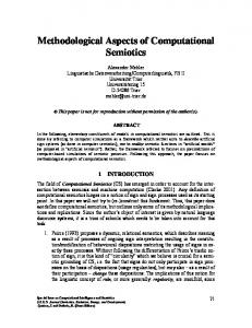
3.4.4 Performance considerations Using PMCD and the radionuclide transport model GTMCHEM, we made a Monte Carlo simulation with 1000 runs to study the performance of PMCD. Table 3.4.1. and Figure 3.4.2 shows the results of the performance test. Increasing the number of processors from 2 to 12 resulted in a CPU time gain of approximately one order of magnitude. From 12 to 26 nodes one gets a further gain of roughly 50% between the last two steps. For 1000 realisations there is clearly no advantage to increase the number of nodes further, because the benefit of increasing that number is balanced by intercommunication costs between the nodes. The performance of the PMCD code is dependent upon the type of deterministic code coupled to it and also upon the total number of realisations. Whenever massive production runs are planned the user should make a preliminary estimate to determine the number of nodes that are to be used. For instance, for one million realisations for the same scenario as above (same input data) we obtained a total execution time of circa 4 hours using 25 nodes (see Figure 3.4.3). Considering that we increased the number of realisations by three orders of magnitude, we got a total time which was more than one order of magnitude lower than could be expected from Table 3.4.2.
Nodes
Time [s]
2
40872
4.8 4.6
11
10432 4455
16
3124
21
2457
26
2051
31
1801
36
1601
4.4
Execution times [s]
5
4.2 4.0 3.8 3.6 3.4 3.2 3.0 0
5
10
15
20
25
30
35
40
Nr. of nodes
Figure 3.4.2. Execution times performance. Execution times are plotted in log-scale.
Table 3.4.1 First performance tests.
35
Reference Scenario - Histogram of 1.000.000 runs
No of obs
89840 84225 78610 72995 67380 61765 56150 50535 44920
I-129
39305 33690 28075 22460 16845 11230 5615 0 -9.8
-9.3
-8.8
-8.3
-7.8
-7.3
-6.8
-6.3
-5.8
-5.3
-4.8
Dose [Sv/yr]
Figure 3.4.3. The dose distribution for the reference scenario is close to the theoretical log-normal distribution. Observe that the x-axis has a logarithmic scale.
In the next table we have collected the performance data for the LEVEL E/G exercise. The table shows the number of nodes and execution time for each scenario.
Scenario
Iodine Time
Nº of nodes
[minutes]
Chain Total time
Time
[minutes]
[minutes]
Nº of nodes
Total time
[minutes]
173.8
5†
869
70.3
36†
2530.8
E.I.C.
10.4
4‡
41.6
68.55
25†
1713.7
F.P.
1.18
4‡
4.7
26.9
5†
134.5
G.A.
14.4
4‡
57.6
189
36†
6804
H.D.E.
33.7
4‡
134.8
94.7
25†
2367.5
Ref.
2.35
4‡
9.4
87.6
10†
876
†
A.G.
‡
These nodes are batch nodes. All other nodes are interactive nodes. The batch nodes are nodes solely dedicated to the simulation. The interactive nodes are shared nodes and the execution time may have strong variations from node to node.
Table 3.4.2. Number of nodes and execution time for each scenario. Level E/G
36
Overall the computations for LEVEL E/G exercise with the present set of model parameters are relatively light for the power of the computer we used (IBM SP2). Observe for instance that 1000 runs for the 129I radionuclide are done in less than 3 minutes with four interactive nodes. But another observation is in order: the performance of the simulations is very sensitive to the values of some of the parameters. For instance it was observed that changing the range of the pdf for the VREAL parameter (interstitial velocity) in the third layer, from [0.5 - 1.0 m/yr] to [5.0 - 10.0 m/yr] of the A.G. scenario, caused a worsening of execution time of over 500%. The range used during the exercise was the first one.
3.4.5 Correlation between parameters in Monte Carlo calculation The main results of probabilistic simulations done with the help of the PMCD code are integrated in the sections devoted to the LEVEL E/G calculations, UA and SA. In this section we include only some extra calculations in which the goal is related to one important issue in Monte Carlo simulations of radionuclide migration: correlations between parameters sampled from input distributions. In simulations of complex ecosystems, models describing these systems often include parameters that are correlated with each other. Codes for Monte Carlo simulations of radionuclide transport (Prado, Saltelli and Homma 1991) sometimes make it possible to induce rank correlations between parameters using the method of Iman and Conover (1982). The PMCD code can cope not only with correlations between parameter ranks but also with correlations between the parameters using another approach. This last approach avoids the loss of information that the transformation of parameters to their ranks imply (Pereira and Sundström 1998). The impact of this loss is difficult to predict a priori, but experience suggests that correlation between ranks is sufficient in many cases. It was not necessary for PMCD to induce correlations in the LEVEL E/G exercise. It is therefore illustrated here only for the sake of completeness. The calculations were done using a small number of realisations (500) for the case of iodine migration in the reference scenario of LEVEL E/G. The parameters that were correlated were the interstitial velocity of the second layer and the dispersion length of the same layer. We assume that there exists a stochastic correlation between those two parameters with a negative correlation value between the pdf´s from which those parameters are sampled. That value is given by ρ = -0.5 where ρ is the Pearson´s correlation coefficient. Figure 3.4.4 and Table 3.4.3 show the results obtained.
37
Scatterplot with Histograms 112
56
0
Dispersion length [m]
20 17 15 12 10 7 5 2 0.010
0.024
0.038
0.051
0.065
0.079
0.093
0
44
88
Intersticial velocity [m/yr] Figure 3.4.4. Scatter plot of the interstitial velocity versus the dispersion length of the second layer together with the distributions of the two parameters. A Pearson correlation value equal to -0.45 was obtained by the correlation entropy solver subroutine of the PMCD code. Correlation matrix Contim Rleach
Vreal(1) Xpath(1) Ret(1)
Vreal(2) Xpath(2) Ret(2) Stream
Dispc(2)
Contim
1.0
-.01
.07
.02
-.01
-.12 *
-.01
.00
-.04
.05
Rleach
-.01
1.0
-.04
.01
.02
.10 *
.03
-.03
.01
-.03
Vreal(1)
.07
-.04
1.0
.07
.03
-.02
-.01
.05
.04
.00
Xpath(1)
.02
.01
.07
1.0
.04
-.00
-.01
-.00
-.02
-.02
Ret(1)
-.01
.02
.03
.04
1.0
.02
-.00
.01
-.08
-.02
Vreal(2)
-.12 *
.10 *
-.02
-.00
.02
1.0
.05
.03
.02
-.45 *
Xpath(2)
-.01
.03
-.01
-.01
-.00
.05
1.0
.03
-.04
-.06
Ret(2)
.00
-.03
.05
-.00
.01
.03
.03
1.0
-.01
-.02
Stream
-.04
.01
.04
-.02
-.08
.02
-.04
-.01
1.0
-.02
Dispc(2)
.05
-.03
.00
-.02
-.02
-.45 *
-.06
.03
-.02
1.0
* These correlations are significant at p < .05
Table 3.4.3. Pearson correlation coefficients between input parameters. The desired correlation value equal to -0.5 between the considered parameters is within the expected error band. 38
4
GLOBAL APPROACH IN GESAMAC. THE LEVEL E/G TEST CASE
In order to test and demonstrate the methodology proposed by GESAMAC, at the end of the first project year (GESAMAC 1996) a test case was outlined. Prior to agreeing the final specifications of the test case, the partners and the Commission met frequently. Once the specifications were settled, the four teams involved in the project performed two separate sets of runs. The aim of the test case was to perform Monte Carlo simulation of a hypothetical radioactive waste disposal system in order to produce a set of model realisations that could be used for sensitivity analysis and assessment of model uncertainty. This section describes the specifications of the test case, the simulations performed, the results and our conclusions.
4.1 LEVEL E/G. GENERAL FRAMEWORK In January 1985 the Probabilistic System Assessment Code (PSAC) User Group was established by the NEA Radioactive Waste Management Committee (RWMC) to help coordinate the development of probabilistic safety assessment codes in Member countries. One of the main tasks carried out by the Group was its development of cases studies that tested and verified the models and tools used by different countries and teams. One of these test cases was the Level E exercise. Preceded by the PSACOIN Level 0 (NEA PSAC, 1987) exercise, which focused on testing the “executive” modules of a PSA code, the Level E test case concentrated on the geosphere sub-model. It included an ‘exact’ (hence E) solution which permits code verification. Since then, this exercise has been partially used to carry out other test cases (NEA PSAC Level S 1993) in numerous studies by different teams around the world. To summarise, the PSACOIN Level E is a documented and well-established test case. The Level E/G test case is an extension of Level E adapted to the GESAMAC purposes (hence the last G). PSACOIN Level E evaluates parametric uncertainties for a central scenario and examines the validity of structural assumptions. Level E/G retains the original Level E specifications and incorporates scenario and structural uncertainties (specifically, conceptual model uncertainty) into the analysis.
4.2 OBJECTIVES OF THE LEVEL E/G TEST CASE The exercise was proposed for the first time at the end of the project’s first year, when a preliminary draft of the test case was presented and discussed (Prado 1996). Aiming to promote collaboration and the exchange of knowledge between the different teams in the project, the Level E/G test case was specifically intended 1. to test individual methodologies and tools developed (or used) by each team; 2. to establish links between the four different areas of interest in GESAMAC; and 3. to perform a first global trial of the whole GESAMAC project. Based on the PSACOIN Level E test case conducted in 1989 by the PSAC UG, the new test case attempts to carry out an exercise integrating all kind of uncertainties by considering a set of alternative scenarios associated with different structural assumptions, and characterised by different variables and/or parameter values. The disposal system addressed in the Level E/G test case is a generic one. When reference is made in the text to existing assessments from - for example - AECL or TVO, this is done only by way of comparison, without pretension of extracting or extrapolating from actual data. All the data used in GESAMAC are 39
synthetic, starting from the base case up to the kinetic and filtration constants that were used for some of the scenarios. As the project title suggests, the purpose of GESAMAC is to offer conceptual and computational methodological improvements to usual practice. It is not the purpose of GESAMAC to suggest novel data for the filtration constant of Np in caolinitic media, but to show how this mechanism can be incorporated into the analysis, and how faulting scenarios can be combined into an assessment. For an actual assessment of a site-specific disposal there will be teams devoted specifically to the characterisation of the geochemistry of the site. Subsequent sections describe the procedure followed to define the test case: how the alternative scenarios and the structural and model assumptions were established, and how the scenario probabilities were assigned. They are followed by a description of the simulations performed, looking at the peak doses and total doses at specific time points. Finally we report the results and the conclusions achieved.
4.3 SCENARIO APPROACH The reference case (PSACOIN Level E) considered a central scenario with particular structural assumptions for the model; i.e., it focused on parametric and predictive uncertainties. The new test case intends to perform a fully quantitative synthesis of all sources of uncertainty (scenarios, structural, parametric and predictive) present in performance assessment studies for nuclear waste disposal systems. Therefore, the exercise proposed needs to define a reduced number of scenarios connected with different structural assumptions and/or parameters and/or processes. Moreover, each scenario is associated with a probability of occurrence, taking into account that the total probability over the scenarios considered must be one. If we consider by scenario any possible and conceivable evolution of the system of interest, an unlimited number of possible scenarios can be postulated. Therefore, for practical reasons, the number of scenarios for analysis must be limited to a small set that are of particular interest. Usually the chosen scenarios were those which, in principle, could be expected to have a higher impact, either in terms of probability or consequences. In recent years different strategies and procedures have been followed around the world to identify, structure, select and combine the Features, Events and Processes (FEPs) of interest for safety assessment studies (AECL-92, SITE-94, TVO-92, etc.). Some of the methodologies proposed are the Sandia Methodology (based on fault and event trees), the Rock Engineering Systems (RES) methodology (SKB, TVO, BIOMOVS), and the Process Influence Diagram (PID) technique (SKI Site-94). The relevance of scenarios in radioactive waste performance assessment (and/or safety assessment) studies is being guided by the OECD/NEA, and is aimed at the creation of an international FEP database. However, it is not the scope of this document to discuss the different methodologies or approaches followed for scenario development in the safety assessments studies published during in recent years in the open literature. On the contrary, for the purpose of the exercise proposed, a reduced number of scenarios is sufficient, independent of which methodology is followed for their definition. The procedure followed in GESAMAC for scenario selection included the following three steps: 1. Select a reduced number of generic scenarios called macro-scenarios 2. Choose a reduced number of possibilities within each macro-scenario category, called microscenarios
40
3. Merge micro-scenarios with similar model conceptualisation into a final list of scenarios for simulation.
4.3.1 Macro- and Micro- Scenarios The macro- and micro-scenarios selected for the test case are described below. Apart from the normal evolution scenario, which corresponds to the specifications of the PSACOIN Level E test case, for each macro-scenario three different alternative configurations were considered. Then, similar configurations from different scenarios were grouped for simulation purposes, resulting in a final list of five alternative scenarios to the reference case. 4.3.1.1
Reference Scenario (Level E from PSAG)
This scenario can be associated with present day conditions maintained over time. It assumes that all system barriers will perform the tasks for which they were designed, and in our case it corresponds with the original PSACOIN Level E specifications. In the following pages, we refer to it as the 'central case' or 'reference case'. 4.3.1.2
Geological Scenarios
Under this heading, we address possible changes in the system evolution related to geological processes and/or phenomena. Here we concentrated our attention on a particular geological scenario, the faulting scenario. As result of the local/regional tectonic activity, a new fracture arises in the repository area, or an old fracture is reactivated. Three different micro-scenarios have been postulated: G1.
Fault passing through the vault (direct pathway to the biosphere)
G2.
Fault passing some meters away from the repository (travel time reduced)
G3.
Fault passing far away from the repository (induced changes into the physico-chemical environment)
G1
G2
G3
Figure 4.3.1. Geological Micro-scenarios 4.3.1.3
Climatic Evolution Scenarios
The long time periods needed for radioactive waste disposal systems studies imply changes in the climatic environment of the system. Climate evolution, in most of the safety case studies, concentrates on glacial pulses predicted by the climatic models through the next 120,000 years (including or excluding warm periods). The length of glacial phases has averaged 100,000 years with short interglacial phases of about 10,000 years. Climatic models predict different pulses for the next glacial phase with cold periods at 5, 20, 60 and 100 thousand years. (TVO-92).
41
From a safety point of view, the most significant effects of glaciation are related to changes in the boundary conditions, the deformation of the earth’s crust, fluctuations in sea level, the potential increase of the hydrostatic pressure, changes in flow and chemistry of the groundwater and drastic changes in the biosphere. The final effects can be seen through changes in the system’s environmental conditions. In principle the magnitude of such changes would increase from the vault to the biosphere. In theory, during a glacial cycle, the average recharge rate from surface to groundwater is reduced. However, there may be areas with free pressurised water at the bottom of the glacier, which can be infiltrated. Melting of glaciers simply releases the precipitation that has accumulated in them over the glacial phase. During melting phases there may be strong fluctuations in the flow of groundwater. Some studies have conceptualised this transient phase as a “short circuit” of the transit time of groundwater from the vault into the biosphere. However this increase in the groundwater flow is compensated for by the dilution capacity of the surface waters (TVO-92). On the other hand, glacial melt waters are oxidising, non-saline and have low content in humic substances. Most of the oxygen will be consumed by the surface layers (provided there is not a high conductivity fracture to the vault) and therefore important changes in groundwater chemistry are not expected (TVO92). The alternation of cold and warm periods can be interpreted from the point of view of safety analysis as transient phases, accompanied by accumulation and rapid transport of pollutants respectively. From the point of view of groundwater transport, accumulation periods could be associated with transport that is mainly diffusive, whereas warm periods should be governed by advection as the dominant process. Glaciers transport important amounts of materials away from the areas through which they pass, then deposit them when and where the energy of the ice decreases. Based on the position of the site relative to the glacial front, we can expect two possible cases. When the site is close to the ablation area (warmer periods) of the glacier, an additional geosphere layer can be formed when the ice comes back (till deposits). Alternatively, if the site is behind the glacial front, instead of deposition, the erosion processes could have partially removed the upper geosphere layer, and therefore the total geosphere path length could be reduced. In conclusion, the following micro-scenarios have been considered: C1. Fast pathway from the vault to the biosphere. The geosphere barrier is partially removed by erosion. C2. Glacial retreat (total head increase with depth). This corresponds to an accelerated discharge during long-term glacial retreat associated with an increase in Darcy velocities as a result of the increased gradients. Ground water flow direction is upwards. C3. Glacial advance (total head decrease with depth). This represent the opposite situation to scenario C2 and concerns a period of infiltration during long-term glacial advance. Darcy velocities increase but, in this case, flow direction is downwards.
42
C1
C2
C3
Figure 4.3.2. Climatic Micro-scenarios
Ice motion
Ice motion
Figure 4.3.3. Schematic illustration for scenarios C2 and C3 (SKI SITE-94, 1996) 4.3.1.4
Human Activities Scenario
This macro-scenario includes the effects associated with anthropogenic activities, from the incorrect disposal of wastes into the vault through to direct and/or induced changes in parts of the system resulting from human activities until there is direct intrusion into the vault. Although some safety studies do not consider human intrusion scenarios, and/or they prefer to perform a separate study, for the objectives of the current test case, three alternative micro-scenarios have been considered H1.
Human intrusion bypassing some barriers, mainly identified with human activities like mining or drilling of a pumping well (the worst case will be the direct intrusion)
H2.
Human disposal errors; comprising deficiencies in construction of the facility, in the waste disposal operations, in the emplacement of the multibarrier system, etc.
H3.
Environmentally induced changes; referring to a variety of human activities that result in changes to the system’s environment.
H1
H3
H2
Figure 4.3.4. Human Intrusion Micro-scenarios
43
4.3.2 Micro-Scenarios’ structural assumptions As described in the previous section, three micro-scenarios were established for each of the three macroscenarios. However, from the structural assumptions point of view, and for the purpose of GESAMAC, some of these micro-scenarios could be merged into a single scenario and therefore be studied jointly. The following table shows the micro-scenarios’ merging process up to a final list of five alternatives to the reference case:
G1
G2
C1
C2
H1
H2
FP
AG
G3
C3
H3
HDE
GA
EIC
Figure 4.3.5. Micro-scenario merging process
These five scenarios, in addition to the normal evolution scenario (Level E), depict the final list of scenarios considered in the test case, which are described in the following chapters
C1
G1
FP
Fast Pathway
AG
Additional Geosphere Glacial Advance
H1
C2
G2
H2
GA
C3
G3
H3
HDE
Human Disposal Errors
EIC
Enviromental Induced Changes
Figure 4.3.6. Micro-scenarios merging summary 44
4.3.2.1
(RS) Reference Scenario (PSACOIN Level E)
The system of reference considers a hypothetical radioactive waste disposal system represented by three coupled sub-models: a near field, a far field and a biosphere (NEA PSAC 1989). The repository itself is represented without any consideration of spatial structure or chemical complexities. A small number of representative radionuclides are considered: I-129 and the decay chain Np-237, U-233 and Th-229. The model has a total of 33 parameters, 12 of which are taken as randomly sampled variables. Near Field model. Following the PSACOIN Level E, the source term model consisted of an initial containment time of the wastes (only radioactive decay is considered) followed by a leaching of the inventory present at the time - once the containment fails - with a constant fractional rate. Far Field model. The fluxes from the near field represent the left boundary conditions for the geosphere sub-model. Therefore, the releases of nuclides to the geosphere only depend on leaching rate and inventory in the vault. Then the released radionuclides are transported through the geosphere, represented by a variable number of geosphere layers with different physico-chemical properties. This process was modelled using a one dimensional convective-diffusive transport equation in a semi-infinite porous medium. Biosphere model. A simple biosphere sub-model was considered. Radionuclides leaving the geosphere enter a stream from which the critical group of people obtains drinking water. The doses received depend on the ratio of the drinking water consumption and the stream flow rate.
Level E I-129 Np-237
flow
flow
U-233 Biosphere
Th-229 Source Term
f
Geosphere
Rn
C(0,t) = C 0 e-λt BATEMAN-1
time
f
C(0,t) = C
0Ψ
e-λt e- Ψ(t-t’) BATEMAN-2
t’
time
Biosphere
∂C n ∂ 2C n ∂C n =D −V − R n λ n C n + R n −1 λ n −1 C n −1 2 ∂t ∂X ∂X all X C( X , t ) = 0. t ≤ τ X = 0. C( X , t ) = ' Source_ term' all t
Fi (t ) = β i
w W
L
C i (t )
∂C( X , t ) X = L = 0. ∂X all t
Figure 4.3.7. General view of Level E test case from PSAG UG (OECD/NEA).
45
4.3.2.2 (FP) - Fast Pathway {G1+C1+H1} DCF = 50*LE W = 104 - 106
FP
G1
C1
V = 0,1 - 1 L= 200 - 500 Ri = 1 -2 Rc = 2 - 20
H1
Figure 4.3.8. Fast Pathway Scenario (FP) Near Field model. In the case of a fault (G1), the vault barriers could be broken, followed by an instantaneous release of the remaining inventory at the time of the fault. A glaciation (C1) could be capable of reducing the near field containment time, as a result of the glacial ice overload and the isostatic response of the crust, as well as the possible physico-chemical changes in the environment around the vault following the infiltration of fresh water from the surface, such as increasing container corrosion rates or possible increases in leaching rates. Similarly, unadvertised human activities (H1), like the development of a hole in vicinity of the vault, could partially bypass the natural barriers and modify the environmental conditions around the vault (e.g., flow regime) which would increase leaching rates and reduce containment times. However, time frames for G1 and C1 are in principle longer than the initial containment time. The same can be hypothesised for H1 (no human intrusion before 1,000 years). Therefore, no changes in the reference near field concept are anticipated. Far Field model. In the case of a fault, the geosphere barrier could be partially bypassed. This could be modelled as a new and fast pathway to the biosphere. The fault could be the result of different processes, such as crust accommodation to the global movements of tectonic plates or activation of regional shear zones by glacial load/unload. Another possible effect of glacial phenomena could be the partial or total removal of the upper geosphere layer by erosion, as well as the entrance of surface waters richer in oxygen into the vault area (different chemical processes can be postulated for transport through the geosphere). In the case of human intrusion, the same concept of the system can be postulated, as in the bypass of one of the geosphere layers by mining or drilling activities. In summary, the geosphere system is represented by a fast transport pathway from the vault to the biosphere through the elimination of the upper geosphere layer, the increasing of groundwater, and with new physico-chemical processes in the geosphere transport. The new geosphere layer, characterised by shorter travel times, is represented by a reduced pathlength: only one geosphere, with a faster groundwater velocity. Because of the oxidising conditions due to glacial melt water or by other induced changes into the environment, the retention factors will be reduced. Since it is plausible that clay-altering minerals would be present in fracture surfaces, adsorption by slow reversible reaction is postulated, except in the case of iodine. Equilibrium complexation reaction in solution is also considered. Biosphere model. Although the climatic case considered here could, in theory, be associated with higher dilution factors, it has been assumed that the critical group obtains water directly from a well connected with the fault. Therefore, the dilution factor has been reduced by one order of magnitude from the reference case and the dose conversion factors taken into account are 50 times higher (TVO-92).
46
4.3.2.3
(AG) - Additional Geosphere layer {G2+C2} L = 50 - 100 V = 0,5 - 1 D=3 Ri = 1 - 10 Rc = 4 - 40
AG
G2
V = 10*LE
C2
V = 10*LE
Figure 4.3.9. Additional Geosphere Scenario (AG) Near Field model. The existence of a structure close to the vault area that is very conductive (G2) can, from the system analysis perspective, be translated as a groundwater flow increase combined with changes in the physico-chemical environment around the repository. The effect of the glacial unload by retreat of the glacier (C2) could increase flows around the repository, reducing its containment capabilities and increasing the leaching rates. However, and like the previous scenario, the time scales usually considered for faulting and glacial events expand over the reference containment time, so no changes from the reference near field model are considered. Far Field model. A fault passing some meters away from the vault area could shortcut one or both geosphere layers, and in a similar manner to the near field concept, the environmental properties could change. Since the scenario FP covers partial bypass of the geosphere barrier, here an additional geosphere layer is considered to simulate the fault connecting with the surface. In the glacial case, the supplementary geosphere layer will represent the materials transported and deposited by the glacier in the melting front area, mainly as till deposits. The increase of total head with depth can be associated with changes in the geosphere’s physico-chemical environment. To summarise, the geosphere system is conceptualised as three different layers. The first and second geosphere layers retain the properties of reference case, except for an increase in groundwater velocity. The third geosphere layer is characterised by a length defined by a pdf U: 50-100 m, with a pore velocity represented by LU: 0.5 - 1 m/y, a dispersion length of 3 m and with a higher retention because of the abundance of clay minerals (till deposits for glacial and neoformed minerals for fault cases). The retention factors considered are U: 1-10 and U: 4 - 40 for iodine and the decay chain respectively. Here the chemical processes assumed are equilibrium complexation reaction in solution in all geosphere layers; slow reversible adsorption in the second layer (only for the decay chain); and filtration/biodgradation in the third layer. Biosphere model. We posit no changes from the reference biosphere.
47
4.3.2.4
(GA) - Glacial Advance {C3}
W = 107- 108
GA
L = 50 100 Ri = 2 - 7 Rc = 4 - 40
C3
L= 200 - 600 D=2
Figure 4.3.10. Glacial Advance Scenario (GA) Near Field model. This situation depicts the presence of a thick slice of ice moving over the site area, accompanied by an average recharge reduced to free pressurised water in the bottom of the glacier. The arrival of oxygenated water, in addition to the glacial ice overload, and the isostatic response of the crust can induce changes into the near field environment. However, since the peak of glaciation is expected much later than the initial containment time (Level E), no changes have been considered for the initial vault model. Far Field model. Total head decreases with depth (due to ice sheet thickness over the repository area with the glacial advance), leading to reduced infiltration of oxygenated waters from subglacial melting. Velocities are increased by one order of magnitude relative to the reference case, but in this case flow direction is downwards (SKI, SITE 94), which can be modelled assuming a pathlength increase. In conclusion, in this scenario two layers represent the geosphere system. The length of the first geosphere layer is increased with respect to the reference case. The length of the second geosphere layer is probably reduced by glacial erosion and higher retention factors due to the presence of alteration minerals created by the action of the free pressurised water infiltrating from the bottom of the glacier. We have assumed an equilibrium complexation reaction in solution for all geosphere layers, along with slow reversible adsorption for the second layer (only for the decay chain). Biosphere model. The biosphere probably will be the system where the most important changes can be expected in this scenario; for example, changes in population, human habits, or uses of land. Little surface human activity can be anticipated, however, because the presence of a significant ice sheet would not permit activities like agriculture. Even if there were human settlers in the vicinity, they probably would obtain their resources from places far away from the repository area. If this judgement is correct, the drinking water exposure pathway will not be the most important exposure pathway. It is more probable that external exposure from soil or water, or from eating fish and animals, would be more relevant for dose calculations. Despite these considerations, the reference exposure pathway has been retained but a higher dilution factor was included.
48
4.3.2.5
(HDE) - Human Disposal Errors {H2}
HDE V = 2*LE V = 2*LE H2
C = 50 -500 Yi = 5 * LE Yc = 5 * LE
Figure 4.3.11. Human Disposal Errors (HDE) This scenario includes all human errors associated with repository construction, the disposal of wastes, and other activities related to vault operation. Such errors would be responsible for a premature fault in the near field barriers. Near Field model. The vault is the subsystem directly concerned. The containment time is reduced by a factor of 2 and the inventory leaching rates increased by a factor of 5. Far Field model. Here we use a similar configuration to the reference case. Groundwater velocities increase by a factor of 2 compared to the reference case, reflecting our attempt to incorporate possible induced heterogeneities into the geosphere at the time of the facility construction. We considered two reactions: slow reversible adsorption for the decay chain in all geosphere layers and filtration in the second layer. Biosphere model. This is identical to the reference case. 4.3.2.6
(EIC) - Environmental Induced Changes {G3+H3}
EIC
G3
V = 3*LE Ri = 1 - 3 Rc = 2 - 20
H3
C = 100 - 700 Yi = 3 * LE Yc = 3 * LE
V = 3*LE Ri = 1 - 3 Rc = 2 - 20
Figure 4.3.12. Environmental Induced Changes Scenario (EIC) This micro scenario refers to induced changes in the environmental condition of the repository system. Two different causes are considered as responsible for these changes: a fault and human activities. The first cause is associated with tectonically induced seismicity around the repository area and/or with an important 49
fault far away from the repository area (due, e.g., to major old shear zones). The second cause includes other human activities capable of inducing changes in the properties and/or phenomena operating in the different subsystems of the multibarrier disposal concept. This influence on the system is modelled by induced changes in regional groundwater levels, and therefore in the flow regime around the repository area, and in the physico-chemical reactions and processes involved in the geosphere. Near Field model. Induced changes are translated in the vault system by a slight reduction in the containment time, together with an increase in the leaching rates by a factor of 3. Far Field model. The two original geosphere layers of the reference case are retained. As a result of the arguments mentioned above, the groundwater velocities have been increased by a factor of 3 and the retention factors have been slightly diminished. In this case, the operating phenomena are equilibrium complexation reactions in solution in both layers, slow reversible adsorption in the first layer and biodegradation/filtration phenomena in the second layer. This could occur if, for instance, organic material infiltrated from the surface (or directly introduced by humans) were present. Biosphere model. In theory, no changes from the reference case (Level E) are expected.
4.4 SCENARIO PROPERTIES In this section, each of the final six scenarios described above is characterised by a combination of the following aspects: 1. their probability, 2. the number of geosphere layers, 3. the physico-chemical reactions considered, and 4. the probability distribution functions (pdf's) assigned to the stochastic parameters.
4.4.1 Scenario Probabilities The assignment of probabilities to the different scenarios is a difficult and somewhat speculative task. In fact, the long time periods covered by the safety studies of radioactive waste disposal systems exceeds the age of man; so, the available records of phenomena and events are limited. Therefore the probabilities are speculative. The probability values assigned to the different scenarios described above are synthetic. They have been established by expert judgement. They have been obtained by assigning 90% of probability to the reference scenario and distributing the remaining 10% between the other five scenarios through expert criteria (i.e. scenario S1 is more/less probable than scenario S2, and equal Scenario S3, etc.). Experimenting with those criteria, the final values of probability obtained for the different scenarios are summarised in the following table
Table 4.4.1. Scenario Probabilities
ID.
Scenario
Pronbability
RS
Reference Scenario
0.9000
FP
Fast Pathway
0.0225
AG
Additional Geosphere
0.0125
GA
Glacial Advance
0.0125
HDE EIC
50 Human Disposal Errors Environmental Induced Changes
0,0200 0.0325
4.4.2 Physico-chemical reactions versus scenarios The physico-chemical reactions managed by GTMCHEM computer code and considered in the test case are summarised below: q
Equilibrium Complexation Reaction in Solution
q
Slow Reversible Adsorption
K eq
A + X ↔ AX Sf
A⇔ A * Sb
q
Filtration / Biodegradation
q
Radioactive Decay
q
Linear Retention Factor
β A → λz λb A → B →
A* = Kd A R = 1+
Here A A* X Keq Sf Sb β λ R
radionuclide in solution radionuclide adsorbed phase hypothetical specie in solution equilibrium constant adsorption forward reaction rate adsorption backward reaction rate biodegradation / filtration rate radioactive decay constant linear retention factor (Kd concept)
51
1− ε ρ sKd ε
Np
RNp SNp Np
+
S*Np
λNp RU SU U
λNp
RNpX
λU RTh STh
S* U
βU
X
λNp
UX
RUX
Th
Th
λU
+
βNp
X
NpX
U
I
λTh RI
S*Th
SI S* I I
λTh
+
λI λI
βU
βTh
X
λU
ThX
λTh
RU Th
Figure 4.4.1. Graphical view of the physico-chemical reactions considered in Level E/G Every scenario considers a specific group of such reactions. The following table summarises this information over the scenarios considered in the Level E/G test case.
SCENARIO Reference (Level E) (RS) Fast Pathway (FP) Additional Geosphere (AG) Glacial Advance (GA) Human Disposal Errors (HDE) Environmental Induced Changes (EIC)
Nulcides
1st Layer
2nd Layer
3rd Layer
æ
---
---
---
ž
---
---
---
æ
ECRn+ASR
---
---
ž
ASR
---
---
æ
ECRs
ECRn+ASR
ECRl+B/F
ž
---
ASR
B/F
æ
ECRs
ECRn+ASR
---
ž
---
ASR
---
æ
ASR
ASR + B/F
ž
ASR
ASR + B/F
æ
ECRs+ASR
ECRn+B/F
ž
ASR
B/F
52
Table 4.4.2. Reactions vs. scenarios, nuclides and geosphere layers. Here the acronyms and symbols used have the following meaning:
ASR
Heterogeneous chemical reaction; Adsorption by Slow Reversible reaction between liquid and solid phases
ECR
Homogeneous chemical reaction; Equilibrium Complexation Reaction in solution phase. In order to be more realistic different concentrations of the complexant 'X' are considered at each layer: s = 10-3 n = 10-2 l = 10-1
B/F
Sink reaction; Biodegradation / Filtration / other possible sink reactions
ž for: I129 æ for: Np239 → U235 → Th229
4.4.3 Level E/G Data Set RS Variable Units SUM Micro-sce. Probability Near - field Mol I-129 mols Mol Np-239 mols Mol U-235 mols Mol Th-229 mols Lamb I-129 y-1 Lamb Np-239 y-1 Lamb U-235 y-1 Lamb Th-229 y-1 Tcontain. y Y- Leach-I y-1 Y- Leach-C y-1 1st Geosphere Layer V-GW-1 m y-1 L-path-1 m D-path-1 m RI-129 RNp-239 RU-235 RTh-229 gChain*R Chem proc 2nd. Geosphere Layer V-GW-2 m y-1 L-path-2 m D-path-2 m RI-129 -
FP
AG
Fast pathw. Addit. Geos {GE+C1+H3} {G2 + C2} 0.225 0.0125
GA
EIC
Type
Level-E 0 0.9
C C C C C C C C U LU LU
100 1000 100 1000 4.41E-8 3.24E-7 4.37E-6 9.44E-5 100 - 1000 1E-3 - 1E-2 1E-6 - 1E-5
Idem Idem Idem Idem Idem Idem Idem Idem Idem Idem Idem
idem idem idem idem idem idem idem idem idem idem idem
idem idem idem idem idem idem idem idem idem idem idem
idem idem idem idem idem idem idem idem 50 - 500 idem*5 idem*5
idem idem idem idem idem idem idem idem 100 - 700 idem*3 idem*3
LU U C U C C C U
1E-3 - 1E-1 1E+2 - 5E+2 10 1-5 100 10 100 3 - 30 ---
1 – 0.1. 200 - 500 Idem 1-2 Idem Idem Idem 2 - 20 ECR+ASR
idem*10 Idem Idem Idem Idem Idem Idem Idem ECR
idem 200 - 600 idem idem idem idem idem idem ECR
idem*2 idem idem idem idem idem idem idem ASR
idem*3 idem Idem 1-3 idem idem idem 2 - 20 ECR+ASR
LU U C U
1E-2 - 1E-1 50 - 200 5 1-5
---------
idem*10 Idem Idem Idem
idem 50 - 100 idem 2-7
idem*2 Idem Idem Idem
idem*3 Idem Idem 1-3
53
Glaci. Adv. {C3} 0.0125
HDE
Hum. DIs. Err. Env. Ind. Ch. {H2} {G3 + H4} 0.02 0.0325
RNp-239 RU-235 RTh-229 gChain*R Chem proc 3th. Geosphere Layer V-GW-2 m y-1 L-path-2 m D-path-2 m RI-129 RNp-239 RU-235 RTh-229 gChain*R Chem proc Biosphere wrequire. W stream bI-129 bNp-239 bU-235 bTh-229 ECR ASR B/F
C C C U
100 10 100 3 - 30 ---
-----------
Idem Idem Idem Idem ECR+ASR
LU U C U C C C U
-------------------
-------------------
0.5 - 1 50-100 3 1 - 10 100 10 100 4 - 40 ECR+B/F
m3 y-1 C 0.73 Idem m3 y-1 LU 1E+5 - 1E+7 1E+4-1E+6 Sv mol-1 C 56 5o* Idem Sv mol-1 C 6800 5o* Idem Sv mol-1 C 5900 5o* Idem Sv mol-1 C 1.8E+6 5o* Idem Equilibrium Complexation Reaction in solution Adsorption by Slow Reversible reaction Biodegradation / Filtration
idem idem idem idem idem idem
idem idem idem 4 - 40 ECR+ASR
Idem Idem Idem Idem ASR+B/F
Idem Idem Idem 2 - 20 ECR+B/F
-----------------
-----------------
idem idem idem idem idem idem
idem idem idem idem idem idem
idem 1E+7 - 1E+8 idem idem idem idem
4.5 RUNNING THE TEST CASE The simulation of the test case described above may be performed in two ways: (1) First draw a scenario as random according to the scenario probability distribution previously defined over the six scenarios contemplated. Each scenario is associated with its particular structural assumptions (e.g. number of geosphere layers, chemical reactions involved, etc.). Each scenario and structure are associated with specific variables characterised by their parameter probability distributions, which may be randomly Reference Scenario Important Scenarios Remainning Scenarios
54 Scenario Space
sampled. Then, GTMCHEM generates the model output required by the user in the input file: predicted maximum dose and/or the total dose values at location(s) L and times(s) t. (2) Since the non-reference scenarios have low probability, a more informative sampling strategy is to stratify (over-sample) on them and reweight the results at analysis time, e.g., by making 1000 runs with each scenario. This was our typical method of using GTMCHEM. The simulation performed was focused only on the scenario and parametric components of overall uncertainty.
Figure 4.5.1. From the total scenarios’ space a reduced number are chosen - based on different criteria - for simulation as alternatives to a ’Reference or Central Scenario’. The uncertainty associated with the remaining scenarios that were not considered is redistributed among the scenarios taken into account.
4.5.1 Simulations performed Two separate sets of runs of the test case were performed and analysed. We used the GTMCHEM computer code, which deterministically models the one-dimensional migration of nuclides through the geosphere up to the biosphere: 1- Focused on the total doses versus time (fixed set of time points). The input data sample generated by the JRC team was run by the CIEMAT team and the model outputs obtained were used for sensitivity analysis (i.e. the improved FAST) by the JRC. 2- Focused on the peak doses for the I-129 and Np-239 decay chain separately. The model outputs were generated by the Stockholm University and used by the Bath team to perform SA and model uncertainty calculations. In the first case a total of 5763 model evaluations were performed using three different machines: a CRAY, an IBM workstation and a PC Pentium. The time frame covered by the simulation expands over ten million years, saving the outputs in 40 time points distributed from 103 up to 107 years. In the second case an IBM-SP2 parallel supercomputer was used was used to perform a total of 6000 model evaluations. In this case, each simulation stops once the peak dose has been found. In principle, the first kind of simulation requires more CPU time than the second, because the total time frame (0-107 years) is covered in the first case, whereas in the second the computation stops once the peak dose has been found. On the other hand, we found that certain runs required high CPU times in both cases. In particular, those cases requiring high CPU times were usually associated with the Additional Geosphere and Human Disposal Errors scenarios. This is explained by the time step used to solve the transport equation. The program automatically computes a minimum time step as a function of different properties of the geological media (dispersion and advection) and the physico-chemical constants (radioactive decay, chemical reaction rates and retardation factors) considered. Therefore, the smaller the time step, the higher the total CPU time required.
55
It should also be mentioned that, in order to fully test PMCD, the new parallel Monte Carlo driver, the Stockholm team performed an additional set of evaluations for a fixed set of time points. The output data set obtained is similar to the CIEMAT results described above. They are available on an ftp-server of the Department of Physics at Stockholm University.
4.6 UNCERTAINTY FRAMEWORK IN GESAMAC In the setting described above GESAMAC intends to define a conceptual framework to account for all sources of uncertainty in complex prediction problems, involving six ingredients: -
past data, uncertainty from data collection, measurement, etc.
-
future observables, uncertainties in the new data collected
-
scenario, uncertainty in the plausible future states of the system
-
structural, arising from the different models proposed to explain the system behaviour
-
parametric, arising from incomplete knowledge of the parameter considered
-
predictive, accounting for discrepancies between GTMCHEM outputs and real-world outcomes.
This general categorisation of the system model uncertainties has been transcribed to GESAMAC through the Level E/G application exercise described in the previous sections. The transcription to the hypothetical radioactive waste disposal system considered in the test case has been as follows (see Figure 4.6.1).
Geosphere Inputs (Scenario)
GTMCHEM Chemical Processes (Structural)
Predicted Outputs
Predictive
Chemical Constant (Parametric)
Actual Outputs
Figure 4.6.1. Schematic illustration of the four sources of uncertainty in GESAMAC
•
Past data (D), if available, would consist of readings on radiologic dose under laboratory conditions relevant to those likely to be experienced in the geosphere or biosphere. (Fortunately for humankind, but unfortunately for the creation of a predictive accuracy feedback loop in our modelling - which 56
would allow us to assess the most plausible structural and parametric possibilities - there have been no accidents to date of the type whose probabilities we are assessing.) •
Future observables (y*) consist of dose values at given locations L, t years from now, as L and t vary over interesting ranges.
•
Scenarios (X) detail different sets of likely geosphere conditions at locations L and times t, as a result of human intrusion, faulting, and/or climate. We have found it useful to conceptualise scenario uncertainty in two parts (see Section 4.3): -
Macro-scenarios, consisting of high-level statements of future geosphere conditions relevant to dose, such as climatic change; and
-
Micro-scenarios, which are low-level characterisations of how the macro-scenarios - e.g., how forces of climatic change such as erosion and deposition - would unfold chemically.
•
Structural possibilities (S), include different combinations of chemical processes (e.g., sorption, equilibrium, and matrix diffusion) and different sets of partial differential equations (PDEs) to model them.
•
Parametric uncertainty arises because the precise values of some of the relevant physical constants appearing in the PDEs are unknown. Note that parameters may be specific not only to structure but also to scenario (e.g., an early ice-age climatic scenario would have certain chemical constants driving it, whereas a worst-case geologic fracture scenario would be governed by different constants); and
•
Predictive uncertainty is as speculative (at present) as past data in this project, and might be based on things like discrepancies between actual and predicted lab results, extrapolated to field conditions.
4.6.1 Uncertainty calculations With the six ingredients above, the goal in uncertainty propagation is to produce two types of predictive distributions: scenario-specific and composite. The only hope of doing this in a way that captures all relevant sources of uncertainty appears to be a fully Bayesian analysis (e.g., Draper 1995). In the Bayesian approach past data D (if any) are known; future observable outcome(s) y* are unknown, and to be predicted; and we must pretend that the sets X and S of possible scenarios and structures are known. Then the scenario-specific predictive distribution p(y*/S,x,D) for y* given D, S and a particular scenario x is given by
(
)
(
)
p y * / S , x , D = ∫ ∫ p y * / θ s , S , x p(θ s / S , x, D) p(S / x, D)dθ s dS
(4.6.1)
sθ
and the composite predictive distribution p(y*/S,X,D) for y* given D,S and X is
(
) ∫ p( y
p y* / S , X , D =
*
)
/ S , x, D p( x / D)dx
(4.6.2)
X
Here p(y*/θs,S,x) is the conditional predictive distribution for y* given specific choices for scenario, structure, and parameters, and p(θs /S,x,D), p(S/x,D), and p(x/D) are posterior distributions for the parameters, structure, and scenario (respectively) given the past data. Each of these posterior distributions 57
depends on prior distributions in the usual Bayesian way, e.g., the posterior p(D/S,x) for structure given the data and a particular scenario x is a multiplicative function of the prior p(S/x) on structure and the likelihood p(D/S,x) for the data given structure,
p (S / x, D) = cp( S / x ) p ( D / S , x)
(4.6.3)
where c is a normalising constant.
4.6.2 Challenges to the Bayesian approach This approach to full uncertainty propagation involves two major types of challenges: technical and substantive. -
Technical challenge: Computing with equations (4.6.1-3) above requires evaluation of difficult, often high-dimensional integrals - for instance, the likelihood p(D/S,x) in equation (4.6.3) is p (D / S , x ) = ∫ p( D / θ s , S , x ) p (θ s / S )dθ s
(4.6.4)
θ
and the parameter vector θs given a particular structure S may well be of length l > 50. The leading current technology for overcoming this challenge is (Markov Chain) Monte-Carlo integration (e.g., Gilks et al. 1996, Hammersley and Handscomb 1979). -
Substantive challenges: Q: How can you be sure that X contains all the relevant scenarios, and S contains all the plausible structural choices? A: You can't; in practice you try to be as exhaustive as possible given current understanding and resource limitations. There is no perfect way in this (or any other) approach to completely hedge against unanticipated combinations of events that have never happened before. Q: Where do the prior distributions p(x) and p(S) on scenarios and structures come from? A: One good approach (Dawid 1992, Draper 1997) is to start with expert judgement, use sensitivity analysis (SA) to see how much the final answers depend on these priors, and tune them using predictive calibration: (1) compare the observed outcomes to their predictive distributions given past data - if the observed outcomes consistently fall in the tails, then the priors may have been inaccurately specified, so (2) respecify them and go back to (1), iterating until the predictions are well-calibrated.
4.6.3 A Model Uncertainty Audit How much of the overall uncertainty about maximum dose is attributable to scenario uncertainty, and how much to parametric uncertainty? To answer this question, following Draper (1995), we performed a kind of model uncertainty audit, in which we partitioned the total variance in max dose into two components, between scenarios and within scenarios, the second of which represents the component of uncertainty arising from lack of perfect knowledge of the scenario-specific parameters. The relevant calculations are based on the double-expectation theorem (e.g. Feller 1971): with y as max dose, and scenario i occurring 58
with probability pi and leading to estimated mean and standard deviation (SD) of y of µi and σi, respectively (across the 1,000 simulation replications),
[
] [
]
2 Vˆ ( y ) = VS Eˆ ( y / S ) + Es Vˆ ( y / S ) = σˆ i
= ∑i=1 p i (µˆ i − µˆ ) + ∑i=1 piσˆ i k
2
k
2
(4.6.5)
between whitin = scenario + scenario variance variance
where ∧ ∧ E ( y ) = Es E ( y / S ) = ∑ pi µˆ i =µˆ
4.6.3.1
(4.6.6)
Maximum Dose for the I-129
Table 4.6.1 presents the scenario-specific mean and SD estimates, together with three possible vectors of scenario probabilities. We obtained the first of these vectors by expert elicitation of the relative plausibility of the nine micro-scenarios described at the beginning of this Section, and created the other two, for the purpose of sensitivity analysis, by doubling and halving the non-reference-scenario probabilities in the first vector. Scenario REF FP AG GA HDE EIC
Estimated Mean (µ i) SD (σ i) 2.92e-7 5.63e-7 1.49e-2 2.23e-2 2.47e-6 5.18e-6 4.11e-9 5.96e-9 5.82e-7 1.24e-6 1.17e-6 2.44e-6
Scenario Probabilities (pi) 1 2 3 .90 .80 .95 .0225 .045 .01125 .0125 .025 .00625 .0125 .025 .00625 .02 .04 .01 .0325 .065 .01625
Table 4.6.1. Scenario-specific estimated means and standard deviations of max dose,together with three possible sets of scenario probabilities Table 4.6.2 then applies equations (4.6.5) and (4.6.6) using each of the three scenario probability vectors. It may be seen that the percentage of variance arising from scenario uncertainty is quite stable across the three specifications of scenario probabilities, at about 30% of the total variance1. Scenario Probabilities 1 2 3
Summary
1
In fact, taking the vector of scenario probabilities to be p=(p 1, λp 2) where p 2 is the last five values in the fourth column 5
of Table 4.6.1 and
p1 = 1 − ∑ p 2i , and letting λ vary all the way from 0.01 (corresponding to only 0.001 probability i =1
on the non-Reference scenarios) to 10 (at which point the Reference scenario has zero probability), the proportion of the variance in max dose arising from scenario uncertainty only drops from 30.9% to 25.7%.
59
Overall mean Max dose µˆ Overall SD σˆ Overall varianceσˆ 2
3.36e-4 4.01e-3 1.61e-5 4.90e-6 1.12e-5 30.4 1153 7128
Between-scenario variance Within-scenario variance % of variance between scenarios µˆ / µˆ REF σˆ / σˆ REF
6.72e-4 5.66e-3 3.20e-5 9.57e-6 2.24e-5 29.9 2305 10045
1.68e-4 2.84e-3 8.08e-6 2.48e-6 5.61e-6 30.6 577 5049
Table 4.6.2. Sensitivity analysis of results as a function of scenario probabilities Alternative approaches to the inclusion of scenario uncertainty in risk analysis have been put forward by several investigators: see Apostolakis (1990) as well as a recent special issue devoted to the treatment of aleatory and epistemic uncertainty (Helton et al. 1996). There, predictive uncertainty is partitioned into stochastic (aleatory) and subjective (epistemic), the former corresponding to scenarios and the latter to model structures and parameters in our formulation. An older example of categorisation of uncertainty in risk analysis may be found in Kaplan et al.(1981). Applications to risk assessment for nuclear waste disposal are in Helton et al. (1996) and Helton 1998). Such categorisations, as explained in Apostolakis (1990), are for convenience only, as the two types of uncertainty are indistinguishable in the Bayesian framework. In the present work no distinction is made between scenarios and factors as far as uncertainty is concerned. Table 4.6.2 says that the mean maximum dose of I-129 is 600-1,200 times larger when scenario uncertainty is acknowledged than its value under the Reference scenario, and the uncertainty about max dose on the SD scale is 5,000 - 10,000 times larger. Figure 4.6.2 presents scenario-specific estimated predictive distributions for log maximum dose, and also plots the composite predictive distribution with scenario probability vector 1. The Fast Pathway and Glacial Advance scenarios lead to max dose values which are noticeably higher and lower than the other four scenarios, respectively. Principally because of this, the composite distribution is considerably heavier-tailed than lognormal, in particular including a small but significant contribution of very high doses from scenario FP.
60
Figure 4.6.2. Scenario-specific estimated predictive distributions (top panel) for max dose on the log scale, and composite predictive distribution (bottom panel) using scenario probability vector 1. 4.6.3.2
Maximum Dose for the nuclide chain
Table 4.6.3 and Table 4.6.4 are similar to Tables 4.6.1 and Table 4.6.2 in the previous section, but here they correspond with the results for the Np decay chain of the test case.
Scenario REF FP AG GA HDE EIC
Estimated ) ) Mean ( µ i ) SD(σ i ) 1.21e-7 6.54E-3 8.94E-6 1.20E-9 3.10E-7 1.07E-6
6.25E-7 1.06E-2 1.91E-5 4.72E-9 1.53E-6 4.46E-6
Scenario Probabilities (pi) 1 2 3 .90 .0225 .0125 .0125 .02 .0325
.80 .045 .025 .025 .04 .065
.95 .01125 .00625 .00625 .01 .01625
Table 4.6.3. Scenario-specific estimated means and standard deviations of max dose, together with three possible sets of scenario probabilities.
61
Summary
Scenario Probabilities 1 2 3 1.47E-4 2.95E-4 7.38E-5 2.63E-3 5.66E-3 1.32E-3 6.89E-6 3.20E-5 1.74E-6 9.41E-7 1.84E-6 4.76E-7 2.53E-6 5.50E-6 1.26E-6 27.1 26.7 27.3 1218 2436 610 2980 4201 2110
) Overall mean max dose µ ) Overall SD σ ) Overall Variance σ 2 Between-Scenario Variance Within-Scenario Variance % of Variance between scenarios ) ) µ / µ REF ) ) σ /σ REF
Table 4.6.4. Sensitivity analysis of results as a function of scenario probabilities. It may be seen that the percentage of variance arising from scenario uncertainty is quite stable across the three specifications of scenario probabilities, at about 27% of the total variance. Table 4.6.4 says that the mean maximum dose of the nuclide chain is 600-2400 times larger when scenario uncertainty is acknowledged than its value under the Reference scenario, and the uncertainty about max dose on the SD scale is 2,000-4,000 times larger The information presented in Figure 4.6.3 is similar to the included in the Figure 4.6.2.
62
Figure 4.6.3. Scenario-specific predictive distributions for maximum dose (top panel), and composite predictive distribution with scenario probabilities 1-3 (bottom panel). The scenario probability vector again has little effect.
63
4.7 SENSITIVITY ANALYSIS 4.7.1 . Initial SA results for maximum dose An initial sensitivity analysis was performed for the maximum dose of I-129, which was close to lognormally distributed in all scenarios. We regressed a standardised version of log max dose on standardised versions of scenario-specific inputs, expressed on the raw or log scales as appropriate to produce approximate uniform distributions. All inputs were approximately pairwise uncorrelated. The regressions were well behaved statistically; there was small (not practically significant) evidence of nonlinearity in only one input (VREAL1). As may be seen from the R2 values in Table 4.7.1. nearly all of the variation in log max dose is "explained" by the simulation inputs entered linearly (with no interactions or nonlinear terms). Because the model is so additive in this case, a simple variance-based sensitivity analysis will suffice - more complicated methods are not needed (see next Section 4.7.2). Scenario Nº of Geosphere Maximum Dose Maximum Dose Layers (Min) (Max)
R2
Nº of Model Inputs
REF
2
6,65e-10
5.81e-6
.977
10
FP
1
2.12e-4
1.64e-1
.9998
8
AG
3
6.64e-9
5.89e-5
.982
15
GA
2
3.21e-11
6.35e-8
.961
11
HDE
2
5.06e-10
1.77e-5
.966
14
EIC
2
3.06e-9
2.69e-5
.984
12
Table 4.7.1. Scenario-specific output summaries. Table 4.7.2 gives an example of the regression results, in this case for the reference scenario. When the regression is performed with standardised versions of the outcome y and all of the predictors x j, the squares of the standardised coefficients may be used as a measure of the variation in y (on the variance scale) "explained" by each of the x j provided the predictors are (close to) independent. In this case we have dealt with sample correlations of small size between the x j by averaging the squared standardised coefficients over all possible orderings in which the variables could be entered sequentially into the regression equation. From Table 4.7.2 VREAL1 and STREAM are evidently the high-impact inputs for the Reference scenario. Table 4.7.3 summarises the important variables for each scenario, by retaining only those inputs which “explain” 5% or more of the variance in log max dose. (The standard errors of the standardised coefficients ranged in size from .0041 to .0063; and VREAL1, RLEACH, and STREAM entered the regression on the log scale). It is evident that, apart from occasional modest influence from other variables, the two inputs having to do with water travel velocity play by far the biggest role in the predicted variations in I-129, and in opposite directions: VREAL1 and max dose are positively related (large values of VREAL1 lead to faster travel times through the geosphere to the biosphere), whereas it is small values of STREAM that
64
lead to large iodine doses (arising from less dilution of the fluxes coming from the geosphere to the biosphere). Variable
Standardised Coefficient
Variance in log max dose "explained" by variable
CONTIM
.00151
.000
LRLEACH
-.00261
.000
LVREAL1
.628
.394
XPATH1
-.113
.013
RET1
-.200
.040
LVREAL2
.0676
.005
XPATH2
-.0147
.000
RET2
-.0452
.002
LSTREAM
-.724
.525
"error"
---
.023
Table 4.7.2. Regression results for the Reference Scenario. L at the beginning of a variable name means that variable entered the regression on the log scale.
Scenario
Variable
Standardised Coefficient
Variance in log max dose "explained" by variable
REF
VREAL1 STREAM
.628 -.724
.394 .525
FP
RLEACH STREAM
.419 -.897
.185 .815
AG
VREAL1 STREAM
.593 -.720
.375 .552
GA
VREAL1 RET1 STREAM
.800 -.252 -.478
.645 .063 .229
HDE
VREAL1 STREAM
.633 -.719
.392 .505
EIC
VREAL1 STREAM
.633 -.717
.413 .531
65
Table 4.7.3. Summary of the important variables (those that "explain" 5% or more of the variance in log max dose), by scenario.
4.7.2 SA for the Np-U-Th decay chain In this section we present results for maximum dose of the nuclide chain, obtained by summing max dose across neptunium, uranium, and thorium (thus we are working not with the max over time of the sum across nuclides, maxt [ N (t ) + U (t ) + TH (t )] , but with the sum of the maxes over time, max t [N (t ) ] + maxt [U (t ) ] + maxt [TH (t ) ] , which will in general be somewhat larger). Table 4.7.4 illustrates the inputs to GTMCHEM for the chain modelling in the case of the reference scenario. The max dose distribution was highly positively skewed for all scenarios, motivating a logarithmic transform prior to variance-based SA. For the EIC and FP scenarios log max dose was close to Gaussian, but was negatively skewed in the AG case and appeared to have a two-component mixture form with the REF, GA, and HDE data (see Figure 4.7.1. for the GA case). We do not pursue a mixture analysis here, focusing instead on discovering how much insight simple regression-based methods can provide.
Variable
Meaning
CONTIM
No-leakage Containment time Leach rate after containment failure Geosphere water travel velocity in layer 1 Geosphere layer 1 length Retardation coefficient 1 in layer 1 Retardation coefficient 2 in layer 1 Retardation coefficient 3 in layer 1 Geosphere water travel velocity in layer 2 Geosphere layer 2 length Retardation coefficient 1 in layer 2 Retardation coefficient 2 in layer 2 Retardation coefficient 3 in layer 2
RLEACH VREAL1 XPATH1 RET11 RET21 RET31 VREAL2 XPATH2 RET12 RET22 RET32 STREAM
Distribution
Stream Flow rate
Raw-scale Min Max
Uniform
100
1000
Log-Uniform
1E-6
1E-5
Los-Uniform
1E-3
1E-1
Uniform
100
500
Uniform
300
3000
Uniform
30
300
Uniform
300
3000
Log-Uniform
1E-2
1E-1
Uniform
50
200
Uniform
300
3000
Uniform
30
300
Uniform
300
3000
Log-Uniform
1E+5
1E+7
Table 4.7.4. Example of parametric inputs to GTMCHEM in the simulation study for the radionuclide chain: Reference scenario.
66
Figure 4.7.1. Histogram of standardised log max dose for the GA scenario. We regressed a standardised version of log max dose on standardised versions of scenario-specific inputs, expressed on the raw or log scales as appropriate to produce approximate uniform distributions. All inputs were approximately pairwise uncorrelated. Regressions were less well-behaved statistically (as measured, e.g., by residual plots) than in the case of I-129, on which we have previously reported elsewhere. There was substantial nonlinearity in some scenarios, much (but not all) of which was captured by including quadratic and two-way interaction terms (we explored only quadratics and interactions among the variables with large main effects). As may be seen from the R 2 values in Table 4.7.5, the percentages of “unexplained” variance even after the inclusion of interactions and quadratic terms ranged from 0.9% to 17.3%. Figure 4.7.2 illustrates the non-linearity by plotting the standardised residuals against the predicted values for the HDE data; the dotted curve is a nonparametric smoother, showing that structure remains even after second-order effects of the important predictors are accounted for. Maximum Dose Number of geosphere Scenario layers REF 2 FP 1 AG 3 GA 2 HDE 2 EIC 2
Min
Max
1.33E-11 1.59E-05 2.95E-11 2.66E-12 1.35E-11 2.73E-11
9.18E-06 8.96E-02 2.12E-04 7.03E-08 3.06E-05 6.24E-05
R2 from Main Effects Main + Quadratics Effects + Interactions .770 .827 .967 .991 .832 .943 .685 .884 .847 .923 .864 .907
Number of Model Inputs 13 17 36 25 28 28
Table 4.7.5. Scenario-specific output summaries. Note how much higher the dose is for the FP scenario.
67
Figure 4.7.2. Standardised residuals versus predicted values in the regression of log max dose on main effects, interactions, and quadratic terms, HDE scenario. Dotted line is a robust smoother. Table 4.7.6 gives an example of the regression results, in this case for the Reference scenario. When the regression is performed with standardised versions of the outcome y and all of the predictors x j, the squares of the standardised coefficients may be used as a measure of the variation in y (on the variance scale) “explained” by each of the x j, provided the predictors are (close to) independent. In this case we have dealt with sample correlations of small size between the x j by averaging the squared standardised coefficients over all possible orderings in which the variables could be entered sequentially into the regression equation. From Table 4.7.6 VREAL1 and STREAM are evidently the high-impact inputs for the Reference scenario.
Variable LVREAL1 LSTREAM XPATH1 LVREAL2 RET11 VR1*VR2 VR1*VR1 VR1*XP1 XPATH2 "error"
Standardized Coefficient .622 -.457 -.228 .221 -.191 .184 .170 -.127 -.116 ----
Variance in log max dose "explained" by variable .387 .209 .052 .049 .037 .034 .029 .016 .013 .173
Table 4.7.6. Regression results for the REF scenario. L at the beginning of a variable name means that the variable entered the regression on the log scale. VR1 = LVREAL1, VR2 = LVREAL2, XP1 = XPATH1; X1*X2 = interaction, X1*X1 = quadratic. Only terms
68
whose standardised coefficient exceeded .1 in absolute value are included. The standard errors of the standardised coefficients were all roughly .012. Table 4.7.7 summarises the important variables for each scenario, by retaining only those inputs which “explain” roughly 5% or more of the variance in log max dose. It is evident that, apart from occasional modest influence from other variables, the two inputs having to do with water travel velocity play the biggest role in the predicted variations in max dose of the nuclide chain, and in opposite directions: VREAL1 and max dose are positively related (large values of VREAL1 lead to faster travel times through the geosphere to the biosphere), whereas it is small values of STREAM that lead to large radiologic doses (arising from less dilution of the fluxes coming from the geosphere to the biosphere).
Scenario REF
FP
AG
GA
HDE
EIC
Variable LVREAL1 LSTREAM XPATH1 LVREAL2 LSTREAM LVREAL1 RET1 LVREAL1 LSTREAM XPATH1 VR1*VR1 LVREAL1 VR1*VR1 LSTREAM RET11 LVREAL1 LSTREAM XPATH1 LVREAL1 LSTREAM LVREAL2 XPATH1
Standardized Coefficient .613 -.443 -.217 .216 -.837 .379 -.254 .743 -.384 -.252 -.230 .678 .300 -.289 -.254 .762 -.373 -.246 .713 -.376 .322 -.220
Variance in Log Max Dose "Expained" by Main Effect .376 .196 .047 .047 .701 .144 .065 .553 .147 .063 .053 .460 .090 .083 .064 .581 .139 .061 .509 .142 .104 .048
Table 4.7.7. Summary of the important variables (those that “explain” 5% or more of the variance in log max dose), by scenario. Naming conventions are as in Table 4.7.6.
4.7.2.1
SA via projection-pursuit regression
As Table 4.7.5 indicates, simple regression models with all relevant variables on the log scale - even models that include quadratics and interaction terms among predictors with large main effects - are inadequate to "explain" all of the variance of max dose arising from the radionuclide chain. This suggests either (1) that other variables also play a subtle role in determining log max dose or (2) that the predictors already included have even more highly nonlinear relationships with the outcome of interest. A 69
nonparametric regression technique developed in the 1980s, projection pursuit regression (ppreg; Friedman and Stuetzle 1981), can shed some light on these questions. Given a data set of (univariate) outcomes yi and vectors x i = ( x i1 K xip ) of explanatory variables (for i = 1,K , n ), the idea behind ppreg is to generalise the usual regression model p
y i = µ i + ∑ γ j ( x ij − x j ) + ei ,
(4.7.1)
j =1
in which the e i are IID with mean 0 and variance σ 2 , by replacing the linear manner in which the x j enter the prediction process by arbitrary nonlinear functions of the x j determined nonparametrically: M
y i = µ i + ∑ β mφ m ( a m xi ) + ei , T
(4.7.2)
m =1
Here the a m are unit-length direction vectors onto which the predictors x are projected, and the φ m have been standardised to have mean 0 and variance 1:
[
]
[
]
E φ m (a Tm x) = 0, E φ m2 ( amT x ) = 1, m = 1,K , M
(4.7.3)
In practice the β m , φ m and a m are typically estimated by minimising mean squared error, with the φ functions determined by locally weighted regression smoothing (Cleveland 1979) as in the ppreg function in the statistics package S+ (MathSoft 1998). The extra flexibility of the model (4.7.2) permits discovery of interaction and highly nonlinear relationships between y and the x j , at least in principle. The user must choose M through a compromise between parsimony, interpretability, and explanatory power. As an illustration of this method, we fitted ppreg models to the log max dose data under the REF and HDE ) scenarios. Table 4.7.8 presents the estimated direction vectors a m with the REF data in an analysis with M ) = 2. The predictors in the table have been sorted from largest to smallest in the size of their largest a values, because variables with small weights in both components of the direction vectors cannot play a large role in determining the outcome. One feature of the ppreg method is that simpler models with smaller ) M values are nested within those with larger M, so that the a1 column in this table also provides the ) estimated direction vector with M set to 1. The estimated residual variance with M = 1 was σ 2 =.159, about the same as that from the linear regression model summarised earlier in Table 4.7.6, and the top six ) variables in the a1 column match the important predictors from the previous parametric model, providing some confirmation of the SA for the REF scenario presented earlier. The left panel of Figure 4.7.3 plots the ) ) estimated nonparametric regression function φ 1 ( z1 ) against z1 = a1T x in the M = 1 case; this is approximately quadratic, verifying the earlier result that interactions and squared terms involving the predictors with large linear effects are needed.
70
Variable LVREAL1 LSTREAM LVREAL2 XPATH1 RETC11 XPATH2 RETC12 RETC21 RETC22 RETC32 LRLEACH RETC31 CONTIM
) a1
) a2
.759 -.400 .290 -.278 -.223 -.139 -.102 -.103 -.093 -.039 .034 -.022 .017
-.777 -.334 -.316 .246 .275 .140 .115 .075 .077 .040 -.032 .048 -.008
) ) Table 4.7.8. Estimated direction vectors a1 and a 2 in the ppreg analysis of the REF scenario data with M = 2. L at the beginning of a variable name means that the variable entered the analysis on the log scale.
71
Figure 4.7.3. Estimated nonparametric regression functions φ m (z ) in the ppreg analysis of the REF scenario. The left-hand panel plots φ 1 with M=1; the next two panels plot φ 1 and φ 2 for M=2. However, if one wishes to “explain” more of the output variance, functions more complicated than quadratics are required, as the right-hand panel in Figure 4.7.3 demonstrates. The middle and right panels ) of this figure plot the φ m functions from the M = 2 ppreg solution, and it is evident that something like a ) cubic function of a 2T x would be required to go beyond the M = 1 solution. The corresponding estimated ) weights β m with M = 2 were (.976, .275) - indicating that significant weight is attached to the “cubic” ) component - and the estimated residual variance was σ 2 =.094, about half of its value from the linear regression model summarised in Table 4.7.6. (With these data there is a diminishing return from including more than M = 2 components: the residual variance is still .054 even with M = 9, and only drops to .01 when M ≥ 20 ). This indicates that, even when only two nonlinear components are used, considerably more signal can be extracted via ppreg than with ordinary regression methods. With the HDE scenario a different message emerged. In an attempt to understand the nonlinearity evident in Figure 4.7.2, we fit ppreg models of varying complexity to the HDE data. To obtain a residual variance no ) more than half of the value from linear regression (.077), M ≥ 4 was needed; for example, σ 2 with M = ) 4 was .037. An examination of the a m values to identify important predictors yielded a surprise: in addition ) to the eight variables already spotted with linear regression, four new variables had a m coefficients of at least 0.2. Because this scenario had 28 inputs, it was infeasible in the linear regression modelling to include all possible interaction and quadratic terms; we had contented ourselves with examining only interactions and quadratics among the variables with large linear effects. In this case ppreg was able to identify four additional variables for further study. The main drawback of ppreg for SA seems to be that re-interpreting its nonparametric models in parametric terms may not be easy. For example, while the middle panel of Figure 4.7.3 is approximately linear, a more careful attempt to fit the right-hand panel than that based on a cubic would involve the ratio of two polynomials of at least order 2, and the resulting function of the original variables is a mess.
4.7.3 SA results for total annual dose in the REF scenario Here we describe the results of a sensitivity analysis for total annual dose, arrived at by summing across all four nuclides monitored in Level E/G. It turned out that regression models relating this outcome to the inputs of our simulations were highly non-additive on the raw scale, meaning that simple variance-based methods of the type employed in the previous section were insufficient as a basis for SA in this case. To deal with such situations, we have developed a new method for global sensitivity analysis of model output (Saltelli, Tarantola and Chan 1998) based on the Fourier Amplitude Sensitivity Test (FAST; Cukier et al. 1975). We have named the new method extended FAST because of its ability to evaluate total effect indices for any uncertain factor involved in the model under analysis. The classic FAST is incomplete in characterising the full model behaviour because it can only estimate the first-order (main) effects; the outcomes of the classic FAST are, however, acceptable for additive models. The first-order index for a given factor measures the effect on the output uncertainty due to the variation of the factor itself, over its range of uncertainty, while all the others are allowed to vary simultaneously. The total effect index for a given factor includes the first order effect as well as all the interaction terms involving that factor, thus yielding an overall summary of the factor's influence on the output uncertainty. We argue 72
that each factor has to be described by a pair of indices - first-order and total - and that this kind of representation allows an exhaustive and computationally inexpensive characterisation of the system under analysis. Another method of SA currently employed by many analysts is based on the Sobol' measure (Sobol’ 1990). Although computationally different from extended FAST, we have proved (Saltelli, Tarantola and Chan 1998) that the Sobol' measure and FAST in fact lead to identical SA findings. In other words, the theory underlying FAST, Sobol' and another sensitivity measure, the correlation ratio (Kaplan and Garrick 1981), has been unified. These approaches descend from a common root: the decomposition of the output variance. According to the analysis of variance, the total output variance D may be uniquely decomposed into orthogonal terms of increasing dimensionality, k
D = ∑ Di + i =1
∑D
1≤ i < j ≤k
ij
+ L + D12... k ,
(4.7.4)
where k indicates the number of factors and the terms {Di1 i2 ... is , is ≤ k } are called partial variances. By dividing these terms by D, sensitivity indices (which thus add up to one by definition) can be obtained: Si1 ... is = Di1 ... is / D . Formally, the total effect index for factor i is given by STi = Si + ∑ S ij + ∑ Sijl + L + S12... k j ≠1
(4.7.5)
j