Eurographics Symposium on Geometry Processing (2003) L. Kobbelt, P. Schröder, H. Hoppe (Editors)
Global Conformal Surface Parameterization Xianfeng Gu,1 Shing-Tung Yau2 1
Division of Engineering and Applied Science, Harvard University.
[email protected] 2 Mathematics department, Harvard
[email protected]
Abstract We solve the problem of computing global conformal parameterizations for surfaces with nontrivial topologies. The parameterization is global in the sense that it preserves the conformality everywhere except for a few points, and has no boundary of discontinuity. We analyze the structure of the space of all global conformal parameterizations of a given surface and find all possible solutions by constructing a basis of the underlying linear solution space. This space has a natural structure solely determined by the surface geometry, so our computing result is independent of connectivity, insensitive to resolution, and independent of the algorithms to discover it. Our algorithm is based on the properties of gradient fields of conformal maps, which are closedness, harmonity, conjugacy, duality and symmetry. These properties can be formulated by sparse linear systems, so the method is easy to implement and the entire process is automatic. We also introduce a novel topological modification method to improve the uniformity of the parameterization. Based on the global conformal parameterization of a surface, we can construct a conformal atlas and use it to build conformal geometry images which have very accurate reconstructed normals. Categories and Subject Descriptors (according to ACM CCS): I.3.5 [Computer Graphics]: Surface parameterization, global conformal parameterization
1. Introduction Parameterization is the process of mapping a surface onto regions of the plane. It allows operations on a surface to be performed as if it is flat. Parameterization is essential for many applications including texture mapping, texture synthesis, remeshing, and construction of geometry images. This paper studies conformal parameterization, which c The Eurographics Association 2003. °
is defined in 22, 27, 21 . Conformality of a map equivalently means scaling the metric, it is often described as similarities in the small, since locally shapes are preserved and distances and areas are only changed by a scaling factor 14 . A conformal mapping is intrinsic to the geometry of a mesh 4 , is independent of the resolution of the mesh, and preserves the consistency of the orientation 21 .
Gu et al / global conformal
These nice properties make conformal parametrization suitable for many practical applications. Because of its angle preserving property, conformal parameterization has been proposed for texture mapping 23, 14, 21 , geometry remeshing25 , and visualization 28, 16, 11 . Conformal parameterization continuously depends on the metric of the surface, so it can be used to match two similar surfaces. One such matching method is introduced in 12 . Furthermore, all surfaces can be classified easily by conformal invariants. A method to compute the conformal invariants for meshes is introduced in 12 . Many techniques have been developed to compute conformal parameterizations, but almost all of them only deal with genus zero surfaces and have to segment the surfaces into patches. These methods decompose meshes into topological disks, and then parameterize each patch individually. This introduces discontinuity along the patch boundaries and conformality can not be preserved everywhere. To avoid the problems associated with discontinuous boundaries, global conformal parametrization, which preserves conformality everywhere (except for a few points), is highly desirable. Global conformal parameterization for closed genus zero surface has been addressed in 14, 11, 3, 12 . Global conformal parameterization for closed surfaces with arbitrary genus is investigated in Gu and Yau’s work 12, 10 . Global conformal parameterization for nonzero genus surfaces with boundaries still remains an open problem. This paper solves this problem and discusses its application on constructing geometry images. We also simplify the method introduced in 12 and make the whole process automatic. The algorithms are based on the Riemann surfaces theories 17 . The first figure shows the global conformal parameterizations for surfaces with and without boundaries. 1.1. Contribution We introduce a purely algebraic method to compute global conformal parameterizations for surfaces with nontrivial topologies. To the best of our knowledge, this is the first paper that solves the problem of global conformal parameterization of nonzero genus surfaces with boundaries. Our method of global conformal parameterization has the following properties: • Our method can handle surfaces with arbitrary non zero genus, with or without boundaries. • No surface segmentation is needed. The parameterization is global in the sense that it is conformal everywhere except for a few points and is boundary free. • We find all possible parameterizations. Instead of finding just one solution, we find a basis of the solution space from which all the parametrizations can be constructed. • The method is based on solving large sparse linear systems, by using conjugate gradient method, it can be solved in linear time. We also introduce a way to improve the quality of global parameterizations, namely by modifying the topology of the
model. Furthermore we show how to construct a canonical conformal atlas for closed surfaces. 1.2. Previous Work Surface parameterization has been studied extensively in the graphics field. General methods are based on functional optimization, where special metrics are defined to measure the deviation of the parameterization from an isometry. Tutte introduces the Barycentric maps, and proves the mapping is an embedding in 33 . Floater uses specific weights to improve the quality of the mapping in terms of area deformation and conformality. Levy and Mallet 20 take into account additional constraints to improve the orthogonality and homogeneous spacing of isoparametric curves of the parameterization. Maillot et al. 23 introduce a deformation energy to measure the distortion introduced by the mapping. Levy defines another criterion to measure smoothness and match features in 19 . Hormann and Greiner 15 propose the MIPS parameterization, which roughly attempts to preserve the ratio of singular values over the parameterization. Sander et al. 29 develop a stretch metric to minimize texture stretch and texture deviation. Furthermore, Sander et al. 26 design the signal-stretch parameterization metric to measure the signal error. 1.2.0.1. Conformal parameterization for genus zero surfaces Most works in conformal parametrization only deal with genus zero surfaces.There are four basic approaches. 1. Harmonic energy minimization. Pinkall and Polthier derive the discrete Dirichlet energy in 27 . Eck et al. 22 introduce the discrete harmonic map, which approximates the continuous harmonic maps by minimizing a metric dispersion criterion. Desbrun et al. 25, 4 compute the discrete Dirichlet energy and apply conformal parameterization to interactive geometry remeshing. Levy et al.21 compute a quasi-conformal parameterization of topological disks by approximating the Cauchy-Riemann equation using the least square method. Gu and Yau in 12 introduce a nonlinear optimization method to compute global conformal parameterizations for genus zero surfaces. The optimization is carried out in the tangential spaces of the sphere. 2. Laplacian operator linearization. Haker et al. 14 introduce a method to compute a global conformal mapping from a genus zero surface to a sphere by representing the Laplacian-Beltrimi operator as a linear system. 3. Angle based method. Sheffer et al. 31 introduce an angle based flattening method to flatten a mesh to a planar region so that it minimizes the relative distortion of the planar angles with respect to their counterparts in the three-dimensional space. 4. Circle packing. Circle packing is introduced in 32, 16 . Classical analytic functions can be approximated using circle packing. But for general surfaces in R3 , circle packing only considers the connectivity but not geometry, so it is not suitable for our parameterization purpose. c The Eurographics Association 2003. °
Gu et al / global conformal
(b) Gradient field ω (c) Gradient field ∗ ω (d) A conformal √ gradient field dual to e1 . orthogonal to (b) ω + −1 ∗ ω Figure 1: A conformal gradient field of a two holeRtorus. (a) shows the homology basis, which are four closed curves. (b) shows R the vector field ω dual to e1 , i.e. e1 ω is nonzero, ei ω = 0, i = 2, 3, 4. The shaded curves are the integration lines of the vector √ field. (c) shows the vector field ∗ ω that is orthogonal to (b) everywhere. (d) shows a conformal gradient field ω + −1 ∗ ω. (a) Homology basis
1.2.0.2. Global conformal parameterization for nonzero genus closed surfaces The problem of computing global conformal parameterizations for general closed meshes is first solved by Gu and Yau in 12 . The proposed method approximates De Rham cohomology by simplicial cohomology, and computes a basis of holomorphic one-forms. The method has solid theoretic bases, but it has some limitations of the geometric realization of the homology basis. Each homology base curve can only intersect its conjugate once. Hence the method is not automatic and needs users’ guidance. Also, this method can not handle surfaces with boundaries. The purely algebraic method introduced in this paper is based on the method in 12 , but it has no restrictions on the geometric realization of the homology basis. This method is much simpler and it is automatic. We also generalize this method to handle surfaces with boundaries. 1.2.0.3. Computational topology The computation of homology group and polygonal schema has been studied in 34, 18, 5, 6 . It is shown in 8 that it is NP-hard to compute an optimal polygonal schema with the shortest cut. 2. Basic Idea and Sketch of Mathematical Theories In order to compute conformal maps, we compute their gradient fields first. Each gradient field of a conformal map is a pair of tangential vector fields with special properties. All such vector fields form a linear space. We will show how to construct a basis of this linear space by solving a linear system derived from these properties. We can then get a gradient field of a conformal map by linearly combining the bases. Then by integrating the conformal gradient field, we obtain a conformal parameterization. In this paper, we use the terms gradient fields and conformal gradient fields to refer to the mathematically more rigorous terms closed one-forms and holomorphic one-forms1 . A conformal parameterization maps a local region of a surface √ to the complex plane. We denote its gradient field as ω + −1 ∗ ω, where ω and ∗ ω are real gradient fields. According to Riemann-Roch theory 1 , all such conformal grac The Eurographics Association 2003. °
dient fields form a linear space, whose structure is closely related to the topology of the surface. We use homology group to represent the topology of the surface. All curves on a surface form a homology group as introduced in Appendix A. A homology basis is a set of curves that can be deformed to any closed curves on the surface by operations including replicating, merging, and splitting. We use a set of loops {e1 , e2 , · · · , e2g } to denote a homology basis, where g is the genus. A surface can be cut along a homology basis (a cut graph) to a topological disk, which is called a fundamental domain. Figure 2 (a) demonstrates a homology basis of a genus 4 surface, (b) shows the boundary of its fundamental domain, both of them are manually labelled. The cohomology group is the linear functional space of the homology group, which is defined in Appendix A also. According √ to Riemann surface theory, conformal gradient fields ω + −1 ∗ ω have the following properties: • closedness ω and ∗ ω are closed, meaning the curlix of ω and ∗ ω are both zero. • harmonity ω and ∗ ω are harmonic, meaning that the Laplacian of both ω and ∗ ω are zero. • duality The cohomology class of ω and ∗ ω can be determined by the values of their integration along the homology basis ei ’s. • conjugacy ∗ ω is orthogonal to ω everywhere. According to Hodge theory, given 2g real numbers c1 , c2 , · · · , c2g , there is a unique real gradient field ω with the first three properties, because each cohomology class has a unique harmonic gradient field ω. These properties for ω can be formulated as the following equations: dω = 0 ∆ω = 0 (1) R ω = c , i = 1, 2, · · · , 2g i ei The equation dω = 0 indicates ω is closed, where d is the exterior differential operator; The equation ∆ω = 0 represents the harmonity of ω,R where ∆ is the Laplacian-Beltrami operator; The equations ei ω = ci , i = 1, 2, · · · , 2g restrict the
Gu et al / global conformal
section. We also use u, v, w to denote vertices of M, [u, v] to denote an edge, and [u, v, w] to denote a face. The methods of computing homology basis are described in 24 or 18 . We briefly summarize it here. In our implementation, we compute the eigenvectors of the following matrix ∂T1 ∂1 + ∂2 ∂T2 ,
(a) A homology basis.
(b) The boundary of a fundamental domain Figure 2: (a) and (b) illustrate a topological model for general surfaces. A general surface can be represented as a sphere glued with several handles. Each handle has two special curves, which form a basis of the homology group. Each surface can be sliced open to a topological disk - a fundamental domain. cohomology class of ω. The conjugacy property can be formulated as ∗
ω = ~n × ω,
(2)
where ~n is the normal field on the surface, × is the cross product in R3 . This equation holds everywhere on the surface. The solution ω to equations 1 depends on ci linearly. The linear solution space is 2g dimensional. We can compute a basis {ω1 , ω2 , · · · , ω2g } of the solution space, such that R j j ei ω j = δi , where δi is the Kronecker symbol. Then the solution ω corresponding to {c1 , c2 , · · · , c2g } can be repre2g sented as ω = ∑i=1 ci ωi . This paper uses linear systems to approximate equations 1 and 2 on meshes and automatically computes a basis of conformal gradient fields. Once a conformal gradient field is obtained, we integrate it on a fundamental domain to find a conformal parametrization. For surfaces with boundaries, we apply the double covering method to convert them to closed ones. We get two copies of the surface, reverse the orientation of one of them, and glue them along the boundaries, then obtain a symmetric closed surface. We can compute the conformal gradient fields on the double covering of the surface, and find conformal gradient fields for the original surface with boundaries. Figure 3 demonstrates the base conformal gradient fields, visualized by integrating them on a fundamental domain and texture-mapping a checkerboard image. 3. Algorithm for Closed Surfaces We have just sketched the analytical basis for computing global conformal parameterization. Now we describe a numerical procedure to carry this out. The main task is to transform the mathematical concepts defined on smooth surfaces to operations on triangulated meshes. Assume that M is a triangulated mesh. We continue to use the notation of previous
(3)
where ∂1 and ∂2 are the matrix representation of the boundary operators. ∂1 returns the boundary of a curve, and ∂2 returns the boundary of a patch. The details are explained in Appendix A. Each eigenvector of the null space is a homology base curve. We denote each base as ei , i = 1, 2, · · · , 2g. ei can be represented as a sequence of oriented edges, for example, [u0 , u1 ], [u1 , u2 ], · · · , [un−1 , un ], where un = u0 . Recall √ that a conformal gradient field is represented as ω+ −1 ∗ ω, we approximate ω by a function defined on the edges, and associate each edge with a real number, denoted as ω[u, v]. 3.1. The Real Part of Conformal Gradient Fields This subsection computes the real part ω of the conformal gradient field by using the closedness, harmonity, and duality properties. The closedness property dω = 0 means the integration of ω along any simple closed curve (which bounds a topological disk) is zero. Hence for each face [u, v, w], the integration of ω along its boundary ∂[u, v, w] is zero. Then for each face, the equation for closedness can be approximated by the following linear equation: ω(∂[u, v, w]) = ω[u, v] + ω[v, w] + ω[w, u] = 0.
(4)
The harmonity property ∆ω = 0 can be formulated using the well known cotangent weighting coefficients 7, 4 . For any vertex u, the Laplacian of ω on u is zero, hence the equation for harmonity can be formulated as: ∆ω(u) =
∑
ku,v ω[u, v] = 0
(5)
[u,v]∈M
1 ku,v = − (cot α + cot β) 2
(6)
Figure 3: Visualizations of two base conformal gradient fields by texture mapping a checkerboard. c The Eurographics Association 2003. °
Gu et al / global conformal
where α, β are the anglesRagainst the edge [u, v]. The duality property ei ω = ci can be formulated in a straightforward way. Suppose homology base ei consists of a sequence of oriented edges ei = ∑nj=1 [u j−1 , u j ], where u0 = un , then Z ei
ω=
n
∑ ω[u j−1 , u j ] = ci .
(7)
j=1
The star wedge product ∗ ∧ of ω and τ on smooth surfaces is defined as follows: Z
M
ω∗ ∧τ =
Z
M
ω ∧ ∗τ =
Z
M
ω × ∗ τ ·~n,
(11)
where ∗ τ is obtained by rotating τ about the normal ~n on the tangent plane at each point of M. The discrete star wedge product on meshes is defined as Z
Compared with previous methods in 21, 22, 4, 7 , we have ω ∗ ∧ τ = UMV T , (12) used the duality condition to replace boundary conditions. T By combining equations 4, 5, and 7 together, we get the where discrete version of the system of equations 1: −4l02 l02 + l12 − l22 l02 + l22 − l12 3 1 ω([u , u ]) = 0, ∀[u , u , u ] ∈ M, u = u 2 2 2 2 2 2 2 ∑ j−1 j 0 1 2 0 3 j=1 l +l −l M= −4l1 l1 + l2 − l0 , 1 0 2 24s ∑[u,v]∈M ku,v ω([u, v]) = 0, ∀u ∈ M 2 2 2 2 2 2 l + l − l l + l − l −4l22 2 0 1 2 1 0 ni i i ∑ni ω([ui , ui ]) = c , ∀e = [u , u ], u = u ∑ n i i 0 i j−1 j (13) j=1 j=1 j−1 j (8) and vectors U,V are In order to get a basis of the conformal gradient fields, we U = (ω(d0 ), ω(d1 ), ω(d2 )) (14) choose 2g sets of {ci }, where the jth set is {δij }. In Appendix B, it is proven that the linear system 8 is of full rank. V = (τ(d0 ), τ(d1 ), τ(d2 )). (15) This is the discrete analogue of Hodge theory, which claims We can build a linear system to solve for λi ’s based on the each cohomology class has a unique harmonic one-form rep17 following formula: resentative . Z Z Once we have computed ω, we can compute ∗ ω by using ωi ∧ ∗ ω = ωi ∗ ∧ ω, i = 1, 2, · · · , 2g. (16) the discrete Hodge star operator, which will be introduced M M in the next subsection. Equivalently, we can expand each term, use discrete wedge products and discrete star wedge products to get the follow3.2. The Imaginary Part of Conformal Gradient Fields ing linear system directly Having selected an ω in the space of ω , we compute the i
imaginary part of the conformal gradient field ∗ ω by using the conjugacy property. The Hodge star operator is defined on the gradient fields on smooth surfaces. Intuitively, it locally rotates each vector a right angle about the normal at each point. ∗ ω can be obtained by applying the Hodge star operator on ω. This subsection uses a linear system to approximate the Hodge star operator on triangulated meshes. Suppose {ω1 , ω2 , · · · , ω2g } are a set of basis of all the solutions to linear system 1, then both ω and ∗ ω can be represented as a linear combination of ωi ’s. Suppose ∗ ω = 2g ∑i=1 λi ωi , our goal is to find out λi ’s. Given two gradient fields ω, τ, the wedge product ∧ on smooth surfaces is defined as the following integration Z
M
Z
ω∧τ =
M
ω × τ ·~ndσ,
(9)
where ~n is the normal field of M, dσ is the area element, and the × and · are the common cross product and dot product in R3 . This can be approximated by the discrete wedge product defined below. The details can be found in Appendix C. Suppose {d0 , d1 , d2 } are the oriented edges of a triangle T , their lengths are {l0 , l1 , l2 }, and the area of T is s, then the discrete wedge product ∧ is defined as ¯ ¯ ¯ ω(d0 ) ω(d1 ) ω(d2 ) ¯ Z ¯ 1 ¯¯ ω ∧ τ = ¯ τ(d0 ) τ(d1 ) τ(d2 ) ¯¯ (10) 6¯ T ¯ 1 1 1 c The Eurographics Association 2003. °
W Λ = B,
(17) R
where W has entries wi j = ∑T ∈M ω ∧ ω j , Λ has entries R T i λi , and B has entries bi = ∑T ∈M T ωi ∗ ∧ ω. In appendix D, we show that the linear system 17 is of full rank. 3.3. Conformal Map By solving the linear system in section 3.1, we can compute {ω1 , ω2 , · · · , ω2g }. By solving the linear system in section ∗ 3.2, we can compute {√ ω1 , ∗ ω2 , · · · , ∗ ω √2g }. ∗The conformal ∗ gradient fields {ω + −1 ω , ω + −1 ω2 , · · · , ω2g + 1 1 2 √ ∗ −1 ω2g } are a set of basis of all conformal gradient fields on M. From the finite dimensional space of all possible conformal gradient fields, we can select a desirable one for the application. For example, if we want to optimize the uniformity, we can formulate it as a finite dimensional optimization problem to minimize the L2 norm of the derivative of streching factor function on surface. Once we get the conformal gradient field, we integrate it on a fundamental domain of the surface to get the conformal map. We first compute a fundamental domain of M as described in 12 . We choose one base vertex u0 , which is mapped to the origin of the complex plane. For any vertex v ∈ M, we arbitrarily choose a path from u0 to v in the fundamental domain. Suppose the path is e = ∑ni=1 [ui−1 , ui ], un = v, then
Gu et al / global conformal
the complex texture coordinates of v are Z e
√ ω + −1 ∗ ω =
n
∑ ω[ui−1 , ui ] +
√
i=1
n
−1 ∑ ∗ ω[ui−1 , ui ]. i=1
(18) The complex texture coordinates are path independent, this can be shown by using the fact that both ω and ∗ ω are closed and the Stokes theorem. 4. Surfaces with Boundaries This section generalizes the method for computing conformal gradient fields for closed surfaces to surfaces with boundaries. 4.1. Double Covering Suppose surface M has boundaries, we construct a copy of M denoted as M 0 , then reverse the orientation of M 0 by changing the order of vertices of each face from [u, v, w] to [v, u, w]. We then glue M and M 0 together along their boundaries. The resulting mesh is denoted as M, and called the double covering of M. The double covering is closed so we can apply the method discussed in the last section. For each interior vertex v ∈ M, there are two copies of v in M, we denote them as v1 and v2 , and say they are dual to each other, denoted as v1 = v2 and v2 = v1 . For each boundary vertex v ∈ ∂M, there is only one copy in M, we say v is dual to itself, i.e. v = v. 4.2. Symmetric Conformal Gradient Fields We now compute the conformal gradient fields of M. According to Riemann surface theories 30 , all symmetric conformal gradient fields of M restricted on M are also conformal gradient fields of M. The real part of a symmetric conformal gradient field satisfies the following property: ω[u, v] = ω[u, v].
(19)
We can simply perform the process described in the last section on M: compute homology basis of M; compute ωi ’s; √ compute ∗ ωi ’s. Then ωi + −1 ∗ ωi s are a set of basis of all conformal gradient fields on M. Define the dual operator for each gradient field ω as follows: ω([u, v]) = ω([u, v]), ∀[u, v] ∈ M.
(20)
The dual operator exchanges the numbers a gradient field associates with an edge and its counterpart in the double covering. Then any ω can be decomposed to a symmetric part and an asymmetric part: 1 1 ω = (ω + ω) + (ω − ω), 2 2
(21)
where 12 (ω + ω) is the symmetric part. √ Given a conformal gradient field√ω + −1 ∗ ω on M, the symmetric component 21 (ω + ω) + −1 12 ∗ (ω + ω) is also a conformal gradient field of M. If we restrict it on M, then √ 1 1 { (ωi + ωi ) + −1 ∗ (ωi + ωi )} (22) 2 2
(a) Zero point of the open teapot (b) Zero point of f (z) = z2 Figure 4: Zero points of parameterization. are a set of basis of conformal gradient fields on M. 5. Global Conformal Atlas In the last two sections, we have introduced a method to compute conformal gradient fields for general surfaces, and by integrating a conformal gradient field on a fundamental domain, we can conformally map the surface to the complex plane. This section analyzes the global structure of the image of a conformal mapping. For a general surface M, each handle of the surface is conformally mapped to the complex plane periodically, where each period is a parallelogram. The set of such parallelograms for g handles is the global conformal atlas of M. If the surface is of genus one, then the mapping is one-toone. Otherwise, the mapping is in general one-to-one locally, but there are 2g − 2 special points that are called zero points. In the neighborhood of zero points, the mapping has special structures. The local structure of the zero points is explained below. 5.1. Zero Points According to the Poincare-Hopf index theorem 13 , a conformal gradient field ω must have zero points if M is not homeomorphic to a torus. Zero points of ω are the points where the mapping is degenerated. According to Riemann-Roch theory, there are totally 2g − 2 zero points for a genus g surface. The map wraps the neighborhood of each zero point twice and double covers the neighborhood of the image of p on the complex plane. Locally, the map is similar to the following map f : C → C in the neighborhood of the origin: f (z) = z2 .
(23)
Figure 4 demonstrates the zero points on the global conformal parameterizations. For the open teapot model, its double covering is of genus two. There are two zero points, one of them is illustrated near the bottom. In order to find the zero points, we define the following stretching factor for each vertex u ∈ M, s(u) =
1 ||ω[u, v]||2 . ∑ valence(u) [u,v]∈M ||[u, v]||2
(24)
c The Eurographics Association 2003. °
Gu et al / global conformal
(a) Genus two surface (b) Conformal atlas of (a) (c) Genus three surface (d) Conformal atlas of (c) Figure 5: Global conformal atlas. For a genus g surface, there are 2g − 2 zero points. We pair them to g − 1 pairs, and construct a loop to go through each pair. These loops separate the handles. Each handle is mapped conformally to a modular parallelogram. The conformality is preserved across all the boundaries. The grey disks show the modular structure of each handle, the grey line segments are handle separators, the white disks show that conformality is preserved across the handle separators. The minimum points of s(u) approximate the positions of the zero points. 5.2. Modular Structure of Each Handle Given a topological torus M and a conformal gradient field ω on it, we pick a base point u0 and issue curves from u0 arbitrarily to any point on the surface. By integrating ω along these curves, we map M to the plane conformally. The curves can be extended to infinity, and the mapping can also be consistently extended. The image set of the base point is Z
{a e1
Z
ω+b
e2
ω|a, b ∈ Z},
(25)
where {ei } are homology basis curves. The mapping is periodic or modular. Then the entire torus is conformally mapped to one period, which is a paralleloR R gram spanned by e1 ω, e2 ω. The top and bottom of the parallelogram are identical, the left and right are identical, and the four corners are identical. We call this parallelogram a modular space and use it as the global conformal atlas of M. R R We call { e1 ω, e2 ω} the periods of M. Suppose the genus of M is greater than one, then we can still map each handle to a modular space, but now different handles may have different periods. The entire surface is mapped to g overlapping modular parallelograms. Two parallelograms may attach to each other through the images of zero points, and cross each other between the images of the zero points. We can separate the parallelograms, therefore separate the handles. As shown in figure 5 (a) and (b), the two-hole torus is separated into two handles, and each handle is conformally mapped to a modular space. The mapping across the boundary is still conformal. The grey disks on the two handles in (a) are mapped to the modular spaces in (b); this illustrates the modular structure of the conformal parameterization of each handle. (c) and (d) demonstrate a global conformal parameterization of a genus three torus. From (d) we can tell that each handle has different period. c The Eurographics Association 2003. °
The grey line segments in the interior of each modular space are the images of the closed curves which separate different handles, and they are called handle separators. The ending points of the handle separators are zero points. The next subsection will explain how to find the handle separators. 5.3. Handle Separation For general surfaces M with genus higher than one, by integrating ω on a fundamental domain, M is conformally mapped to g overlapping modular parallelograms on the complex plane. This subsection discusses how to separate these parallelograms to construct the global conformal atlas. Suppose the conformal mapping is f . Between two adjacent handles on M, there are two zero points, p0 and p1 . We can always find a closed curve that goes through them and separates the handles. We denote the curve segment from p0 to p1 as [p0 , p1 ], and the curve segment from p1 to p0 as [p1 , p0 ]. Then ~f maps [p0 , p1 ] and [p1 , p0 ] to the same curve segment on the plane. We call this kind of curves handle separators. In figure 5, the handle separator is shown on the two-hole torus as the boundary of two regions. It is mapped to the line segments on the modular spaces in (b). The mapping is conformal across the handle separator. The white disk in (a) across the handle separator is mapped to two half disks on the two modular spaces in (b). We can see that the conformality is preserved across this handle separator. Similarly, there are two handle separators in (c), which are mapped to two line segments in the three modular spaces as in (d), the two white disks demonstrate that conformality is preserved across them. The zero points and the handle separators are determined by the conformal gradient field. So handle separation is different from traditional segmentation, which is processed before the parameterization. In practice, we examine the stretching factor of each vertex, and select the minima as zero points. Any two adjacent handles are mapped to two
Gu et al / global conformal
parallelograms, attached by two zero points. We simply choose the line segment connecting the two zero points on these two parallelograms, and their pre-images are the handle separators on the surface. 6. Implementation The implementation of the algorithms is very simple, since it only involves solving sparse linear systems. We use iterative methods to solve them. We use both steepest descendent method and conjugate gradient method. The conjugate gradient method is linear. In order to improve the stability and efficiency, the meshes are preprocessed first. 6.1. Preprocessing In 7 , it is shown that if the mesh has obtuse angles, the discrete harmonic map is not bijective, i.e. local triangle flips may occur. During our numerical experiments, we find that efficiency and stability are related to the positivity of string constants ku,v . Bern et.al 2 introduce a method to triangulate planar regions with non-obtuse angles. For general surfaces with arbitrary topologies, it is still an open problem to triangulate them with all acute angles. In appendix E, we show that all smooth surfaces admit a triangulation with all acute angles, such that all the ku,v ’s are positive. In our implementation, we do some simple preprocessing to remove obtuse angles by heuristic methods. We subdivide the mesh to very fine level, and use edge collapse to remove edges with the minimum lengths to simplify the subdivided mesh. The complexity of the simplified mesh is similar to the original one. After several processes, the angles of the resulting mesh are almost all acute without increasing the complexity of the mesh. 6.2. Topology Modification Conformal parametrizations map surfaces to canonical parameter domains, and encode the three channel geometric information (x, y, z) to one channel stretching factor function. The stretching factor has to be nonuniform. For the extruding parts, such as the ears of the bunny, the stretching factors are highly nonuniform. This is illustrated in figure 8 (a) in color section, when the bunny is conformally mapped to a sphere, the ears parts are shrunk to tiny regions. The corresponding parameterization in (b) indicates the high nonuniformity of this parameterization. Here we introduce a topological modification method to deal with this problem. Because the parametrization is highly dependent on the topology, by punching small holes on the surface, we can change the topology easily without affecting the geometry too much. Generally, we remove several faces from the extruding parts of the surface manually, for example at the ear tips and the center of the bottom of the bunny, and compute its global conformal parametrization. The results for the bunny are as shown in (c) and (d). The uniformity of the parameterization is improved a great deal. The original surface is of genus zero, after topology modification, it is of genus two.
6.3. Summary of the Process Figure 7 in color section illustrates the process of the global conformal parameterization and the construction of a conformal geometry image 9 for the bunny mesh. Topology Modification First, three holes are punched at the tips of the ears and the bottom of the bunny model in order to improve the uniformity of the parameterization. Double Covering We make two copies of the mesh, reverse the orientation of one of them, and glue them together along the boundaries of the three punched holes. The punched holes and the two copies are illustrated in (a), one of them is displayed as a wireframe. Homology Basis A homology basis of the double covering is shown in (b) as the blue curves. Conformal gradient Field We then solve a set of linear systems 8 and 17 to find a basis of the conformal gradient field space on the double covering. Then we choose the symmetric conformal gradient fields basis 22 on M. Figures (c) and (d) are two such base conformal gradient fields. Conformal Atlas By linearly combining the base gradient fields, we can construct all global conformal parameterizations. We select one with a highly uniform stretching factor function as shown in (e) and map the bunny to the global conformal atlas as shown in (f). From the shading, we can locate the ear, head and body parts. (g) are two geometry images constructed from (f) directly. The geometry images have very good qualities in terms of the reconstructed normals, and regular connectivities, which are shown in (h). 6.4. Results We have applied our method to different data sets, comprising meshes created with 3D modelers and scanned meshes. We tested our algorithm for meshes with different topologies, different resolutions, with boundaries or without boundaries. Figure 6 demonstrates that our algorithm is insensitive to different triangulation and resolutions. A teapot mesh is simplified to reduce the resolution, and the connectivity is also changed. The global conformal parameterizations are illustrated by texture mapping a regular checkerboard. Comparing (a) and (c), we can tell the changes in resolutions and triangulation. (b) and (d) show the similarity of the parameterizations. Figure 9 in color section shows several results for different meshes. (g) is a minimal surface model of genus one with three boundaries. Its double covering is of genus four, with 10k vertices and 20k faces. The most complicated model we tested is the whole body David model (f), the double covering is of genus 16, 365k vertices, 730k faces. This demonstrates the algorithm is robust enough for practical applications. The sculpture model in (h) is of 5k vertices, 10 k faces. The knot model (e) is of 2050 vertices and 3672 faces. 7. Summary and discussion We have introduced a purely algebraic method to compute global conformal parameterizations for surfaces with arbic The Eurographics Association 2003. °
Gu et al / global conformal
(a) Original teapot model
(b) Global conformal (c) Simplified teapot model (d) Global conformal parameterization parameterization Figure 6: Global conformal parameterization algorithm is insensitive to triangulation and resolution.
trary nontrivial topologies, with or without boundaries. This method can be used to compute all possible solutions. Each genus g closed surface can be conformally mapped to g modular parallelograms. The conformality is preserved all over the surface except for 2g − 2 zero points. The parameterization is intrinsic to the geometry only. The canonical atlas constructed in this paper can be used to construct geometry images that have accurate reconstructed normals. In order to improve the uniformity of the parameterization, we have also introduced a topology modification method. According to Klein’s Erlangen program, different geometry branch studies the invariants of a space under different transformation group. The topological structure and Euclidean geometric structure are well studied in computer science. But the conformal structure has not been adequately studied or applied in the field. This paper has introduced a practical method to compute the conformal structures of general surfaces. The holomorphic one-form (conformal gradient field) cohomology group and the periods computed in this paper are the invariants under conformal transformation group. We will continue to research further applications, and improve the efficiency of the algorithms. Appendix A: Homology and Cohomology Let K be a simplicial complex whose topological realization |K| is homeomorphic to a compact 2-dimensional manifold. Suppose there is a piecewise linear embedding, 3
F : |K| → R .
(26)
The pair (K, F) is called a triangular mesh and we denote it as M. The q-cells of K are denoted as [v0 , v1 , · · · , vq ]. A q-chain is a linear combination of q-simplices,
∑
[v0 ,v1 ,···,vq ]∈K
c[v0 ,v1 ,···,vq ] [v0 , v1 , · · · , vq ].
i=0
c The Eurographics Association 2003. °
where ω ∈ C K and σ ∈ Cq+1 K. The kernel of ∂q is Zq K, the image of ∂q+1 is Bq , and the q-th homology group is Hq K = Zq K/Bq K.
(30)
Similarly, the kernel of δ is Z K, the image of δ and the q-th cohomology group is q
q
H q = Z q K/Bq K.
q−1
is Bq K, (31)
Appendix B: Full rank of the linear system of closedness, harmonity and duality In order to prove the nondegeneracy of the linear system of closedness, harmonity and duality, it is sufficient and necessary to show its kernel space is zero only. Suppose we have a homology basis {e1 , e2 , . . . , e2gR }, and a one-form ω, such that ω is closed and harmonic, ei ω = 0, we would like to show that ω ≡ 0. First we want to show the integration of ω on any closed loop is zero. Suppose a curve r is closed, then r can be represented as a linear combination of ei ’s with a 2g patch boundary, r = ∑i=1 ci ei + ∂σ, where σ ∈ C2 . Z r
ω=
2g
∑ ci
i=1
Z ei
Z
ω+
∂σ
Z
ω=
∂σ
ω.
(32)
Because of the closedness condition, the derivative of ω is zero, δω = 0. According to the Stokes theorem, the above equation is ∂σ
(28)
(29)
q
Z
Z
q
∑ [v0 , · · · , vi−1 , vi+1 , · · · , vq ].
δq ωσ = ω∂q+1 σ,
(27)
The set of all q-chains is denoted as Cq K. The boundary operator is a linear map from Cq K to Cq−1 K. Boundary operator ∂q takes the boundary of a simplex, ∂[v0 , v1 , · · · , vq ] =
Because M has a simplicial complex structure, we can compute the simplicial homology H∗ (K, R) and cohomology H ∗ (K, R). We denote the chain complex as C∗ K = {Cq K, ∂q }q≥0 , and cochain complex as C∗ K = {Cq K, δq }q≥0 , where Cq K = Hom(Cq K; R).
ω=
σ
δω = 0.
(33)
Next, we want to show ω is zero. Suppose ω is nonzero at an edge [u, v], assume ω([u, v]) > 0, then we extend the edge [u, v] to a path {v0 , v1 , . . . , vn }, such that ω([vi , vi+1 ]) > 0 and the path can not be extended further. The path has no self intersection, otherwise there is a loop, on which the integration of ω is positive, contradictory to the previous preposition.
Gu et al / global conformal
Let’s examine vn , by construction, the path can not be extended any further, so for any edges [u, vn ] adjacent to it, ω([u, vn ] ≥ 0, with ω([vn−1 , vn ]) > 0. The Laplacian for ω at vertex vn is ∆ω(vn ) =
∑
ku,v ω([u, vn ]).
(34)
[u,vn ]∈M
According to appendix E, we can assume ku,v > 0 for all edges, then the Laplacian at vn is nonzero. Contradiction. So the space of harmonic one-forms is 2g dimensional. Our proof is very general, since we only assume that ku,v are positive. In fact we can prove the following fact, given a functional on all functions from the universal covering space of M to R, (or equivalently a functional on all closed one forms ω = d f ), E( f ) =
∑
ku,v || f (u) − f (v)||2 .
(35)
[u,v]∈M
All the critical points of this functional form a linear space, and the dimension of this space is 2g. For example, if we change the harmonic energy to barycentric energy with ku,v ≡ 1, all the parameterizations with minimum barycentric energy form a 2g linear space. Appendix C: Wedge product Suppose ω and τ are two closed one-forms. We construct local isometric coordinates of a face T = [A, B,C]. A(0, 0), B(a, 0),C(b, c), where a = ||B − A||, b = ||C − A||cosA, c = ||C − A||sinA. ω and τ can be represented as piecewise constant one-forms with respect to these coordinates, 1 (cω[A, B]dx + (aω[A,C] − bω[A, B])dy) (36) ac 1 τ = (cτ[A, B]dx + (aτ[A,C] − bτ[A, B])dy) (37) ac By direct wedge product defined for De Rham one-forms, we get ω =
ω∧τ =
1 (−ω[A, B]τ[C, A] + ω[C, A]ω[A, B])dx ∧ dy.(38) ac
Then
Then suppose T is a face, and the three edges are {d0 , d1 , d2 }, their lengths are {l0 , l1 , l2 } respectively, then Z
T
ω ∧ ∗ τ = UMV T ,
where U = (ωd0 , ωd1 ), V = (ωd0 , ωd1 ), and ¶ µ 1 −l12 − l22 + l02 2l12 M= 8s 2l22 −l12 − l22 + l02
Appendix D: Full rank of the linear system of wedge products Suppose a homology basis is {e1 , e2 , . . . , e2g }, the dual harmonic one-form basis is {ω1 , ω2 , . . . , ω2g }, we would like to show that the matrix R R R ω ∧ ω2 . . . R ω1 ∧ ω2g ω ∧ ω1 R 1 R 1 ω2 ∧ ω1 ω2 ∧ ω2 . . . ω2 ∧ ω2g (45) . . . . . . . . . ... R R R ω2g ∧ ω1 ω2g ∧ ω2 . . . ω2g ∧ ω2g is of full rank. First, we can assume ei ’s are a set of canonical homology basis. That means ei only intersects with ei+g at one point, for all i = 1, 2, . . . , g, as shown in figure 2. Then there exists a fundamental domain D , such that −1 −1 −1 −1 −1 ∂D = e1 e1+g e−1 1 e1+g e2 e2+g e2 e2+g . . . eg e2g eg e2g (46) The wedge product ωi ∧ ω j can be geometrically interpreted as the oriented area of the 4g−gon D embedded in the plane, the embedding is defined as follows: We choose one point as the base point, given a point p ∈ D, find an arbitrary path r from the base to it, then
Z
Suppose τ ∈ Z , then we build the same local coordinates system and represent τ as formula [6], then use the formula of Hodge star, 1
∗
dx = +dy, ∗ dy = −dx.
(41)
Z
f (p) = (
(39)
Because A, B,C are circular symmetric, by circulating A, B,C, we get two similar equations. By adding them together, we get ¯ ¯ ¯ ω[A, B] ω[B,C] ω[C, A] ¯ Z ¯ 1 ¯¯ ω ∧ τ = ¯ τ[A, B] τ[B,C] τ[C, A] ¯¯ . (40) 6¯ T ¯ 1 1 1
(43)
Because d0 , d1 , d2 are circular symmetric, by circulating them we get the other two equations. Adding them together, we get U = (ωd0 , ωd1 , ωd2 ), V = (τd0 , τd1 , τd2 ), and −4l 2 l2 + l2 − l2 l2 + l2 − l2 1 2 2 0 2 0 1 2 2 02 22 12 M= l1 + l0 − l2 −4l1 l1 + l2 − l0 24s l22 + l02 − l12 l22 + l12 − l02 −4l22 (44)
Z
1 ω ∧ τ = (−ω[A, B]τ[C, A] + ω[C, A]ω[A, B]). 2 T
(42)
r
ωi ,
r
ω j ).
(47)
It is easy to see (ωi , ωi+g ) will map the boundary of ∂D to a curved square. For (ωi , ω j ), j 6= i + g, ∂D is mapped to two curved segments. This shows Z
j
ωi ∧ ω j = δi+g , i < g, i < j.
(48)
So the matrix 45 is non-degenerated. In general cases, the homology basis is not canonical, then there exists a linear transformation B to map the basis to the canonical one. It is easy to show that the dual harmonic oneform bases can be transformed by B−1 . Wedge product is bilinear, so the new 45 is still nondegenerated. c The Eurographics Association 2003. °
Gu et al / global conformal
Appendix E: Smooth Surface with Triangulation with All Acute Angles We want to prove that each smooth surface admits a triangulation with all acute angles. Here we only sketch the proof for genus zero closed surfaces. Suppose S is a genus zero smooth surface, then S can be conformally mapped to S2 without singularities. A sphere can be triangulated with all acute angles easily, one example is to subdivide an octahedron and map each line segment to a geodesic on the sphere. Then we map this triangulation back to S. Because the mapping is angle preserving, the triangulation on S is also with all acute angles. We can use a mesh to approximate S by changing each curved triangle to a planar one. If the triangulation is dense enough, the planar triangle is very close to the curved one, and each angle is acute. For surfaces with higher genus and boundaries, the proof can be conducted in a similar way. Hence, for a smooth surface, we can find a mesh to approximate it, such that the string constant ku,v is positive for each edge. References 1. 2.
3. 4.
5.
6.
7.
8. 9. 10. 11.
12.
13.
E. Arbarello, M. Cornalba, P. Griffiths, and J. Harris. Topics in the Theory of Algebraic Curves. 1938. M. Bern and D. Eppstein. Polynomial-size nonobtuse triangulation of polygons. Int. J. Computational Geometry and Applications, pages 241–255, 1992. X. Gu C. Craig and A. Sheffer. Fundamentals of spherical parameterization for 3d meshes. In SIGGRAPH 03. M. Desbrun, M. Meyer, and P.Alliez. Intrinsic parametrizations of surface meshes. In Proceedings of Eurographics, 2002. T. K. Dey and H. Schipper. A new technique to compute polygonal schema for 2-manifolds with application to nullhomotopy detection. Discrete and Computational Geometry, 14:93–110, 1995. Tamal K. Dey and Sumanta Guha. Transforming curves on surfaces. Journal of Computer and System Sciences, 58(2):297–325, 1999. T. Duchamp, A. Certian, A. Derose, and W. Stuetzle. Hierarchical computation of pl harmonic embeddings. preprint, 1997. J. Erickson and S. Har-Peled. Cutting a surface into a disk. ACM SoCG 2002. X. Gu S.J. Gortler and H. Hoppe. Geometry images. In SIGGRAPH 02, pages 355–361. X. Gu. Parametrization for surfaces with arbitrary topologies. PhD. thesis, Harvard University. X. Gu, Y. Wang, T. Chan, P. Thompson, and S-T. Yau. Genus zero surface conformal mapping and its application to brain surface mapping. In Information Processing Medical Imaging 2003. X. Gu and S.T. Yau. Computing conformal structures of surafces. Communication of Informtion and Systems, December 2002. V. Guillemin and A. Pollack. Differential Topology. PrenticeHall, Inc., Englewood Cliffs, New Jersey, 1974.
c The Eurographics Association 2003. °
14. S. Haker, S. Angenent, A. Tannenbaum, R. Kikinis, G. Sapiro, and M. Halle. Conformal surface parameterization for texture mapping. IEEE TVCG, 6(2):181–189, 2000. 15. K. Horman and G. Greiner. Mips: An efficient global parameterization method. In Curve and Surface Design: Saint-Malo 1999, pages 153–162. Vanderbilt University Press. 16. M. Hurdal, P. Bowers, K. Stephenson, D.Sumners, K. Rehms, K.Schaper, and D.Rottenberg. Quasi-conformally flat mapping the human cerebellum. In Proc.of MICCAI’99, pages 279–286. 17. I. Kra and H. M. Farkas. Riemann Surfaces. Springer-Verlag New York, Incorporated. 18. F. Lazarus, M. Pocchiola, G. Vegter, and A. Verroust. Computing a canonical polygonal schema of an orientable triangulated surface. In ACM SoCG 2001, pages 80–89. 19. B. Levy. Constrained texture mapping for polygonal meshes. In SIGGRAPH 01. 20. B. Levy and J.L. Mallet. Non-distorted texture mapping for sheared triangulated meshes. In SIGGRAPH 98, pages 343– 352. 21. B. Levy, S. Petitjean, N. Ray, and J. Maillot. Least squares conformal maps for automatic texture atlas generation. In SIGGRAPH 02, pages 362–371. 22. M. Eck T. DeRose T. Duchamp H. Hoppe M. Lounsbery and W. Stuetzle. Multiresolution analysis of arbitrary meshes. In SIGGRAPH 95. 23. Jérôme Maillot, Hussein Yahia, and Anne Verroust. Interactive texture mapping. In SIGGRAPH 93, pages 27–34. 24. J.R. Munkres. Elements of Algebraic Topology. AddisonWesley Co., 1984. 25. M. Meyer P. Alliez and M. Desbrun. Interactive geomety remeshing. In SIGGRAPH 02, pages 347–354. 26. S. Gortler P. Sander, J. Snyder, and H. Hoppe. Signal specialized parametrization. Proceedings of Eurographics Workshop on Rendering 2002. 27. U. Pinkall and K. Polthier. Computing discrete minimal surfaces and their conjugate. In Experimental Mathematics 2(1), pages 15–36, 1993. 28. A Tannenaum S Angenent, S Haker and R Kikinis. Conformal geometry and brain flattening. MICCAI, pages 271–278, 1999. 29. P. Sander, J. Snyder, S. Gortler, and H.Hoppe. Texture mapping progressive meshes. In SIGGRAPH 01, pages 409–416. 30. R. Schoen and S.T. Yau. Lectures on Harmonic Maps. International Press, Harvard University, Cambridge MA, 1997. 31. A. Sheffer and E.de Sturler. Parameterization of faceted surfaces for meshing using angle-based flattening. In Engineering with Computers, volume 17, pages 326–337, 2001. 32. Ken Stephenson. Approximation of conformal structures via circle packing. In Computational Methods and Function Theory 1997, Proceedings of the Third CMFT conference, pages 551–582. World Scientific, 1999. 33. W. Tutte. Convex representation of graphs. Proc.London math.Soc., 10, 1960. 34. G. Vegter and C. K. Yap. Computational complexity of combinatorial surfaces. In ACM SoCG 1990, pages 102–111.
Gu et al / global conformal
(a) Punched surface and double covering.
(b) A homology basis
(c) A conformal gradient base. (d) A conformal gradient base
(e) A special conformal gradient (f) Global conformal atlas (g) Conformal geometry image (h) Regular connectivity. field with high uniformity Figure 7: Process of global conformal parameterization and generating a geometry image.
(a) Spherical conformal map of(b) The global parameterization (c) One parameterization with (d) Another parameterization with the bunny mesh. induced from (a) topology modification topology modification Figure 8: Improve uniformity of the global conformal parameterization by topology modification.
(e) Conformal parameterization(f) Conformal parameterization(g) Conformal parameterization(h) Conformal parameterization of genus one surface of genus 16 surface computed by double covering of genus three surface Figure 9: Global conformal parameterization results. c The Eurographics Association 2003. °